| Issue |
A&A
Volume 693, January 2025
|
|
|---|---|---|
| Article Number | A136 | |
| Number of page(s) | 19 | |
| Section | Galactic structure, stellar clusters and populations | |
| DOI | https://doi.org/10.1051/0004-6361/202452602 | |
| Published online | 17 January 2025 | |
Pollution versus diffusion: Abundance patterns of blue horizontal branch stars in the globular clusters NGC6388, NGC6397, and NGC6752★
European Southern Observatory,
Karl-Schwarzschild-Str. 2,
85748
Garching,
Germany
★★ Corresponding author; This email address is being protected from spambots. You need JavaScript enabled to view it.
Received:
14
October
2024
Accepted:
14
November
2024
Abstract
Context. The metal-rich ([M/H] = −0.48) bulge globular cluster NGC 6388 displays a blue horizontal branch (HB). Helium enrichment, which is correlated with changes seen among other light elements, might explain this feature. Conversely, the hot HB stars in the metal-poor globular clusters NGC 6397 and NGC 6752 display high abundances of heavy elements caused by radiative levitation.
Aims. I want to determine the abundances of cool blue HB stars in NGC 6388 to verify whether they are helium-enriched. To exclude the effects of radiative levitation for NGC 6388 and to investigate the abundance changes caused by radiative levitation, I analysed the blue HB stars in NGC 6397 and NGC 6752.
Methods. I obtained high-resolution spectra for all three clusters. I then determined the effective temperatures and surface gravities from UV-optical photometry (NGC 6388) and the spectra (NGC 6397, NGC 6752) together with local thermodynamic equilibrium (LTE) model spectra. The results were used together with equivalent widths by the GALA program, which provides consistent atmospheric parameters and abundances.
Results. For NGC 6397 and NGC 6752, only moderately hot HB stars were suitable for analysis with GALA. When including the literature data, a large scatter is seen at the onset of radiative levitation, followed by increasing abundances up to about 13 500 K (Si, Fe), then turning to a plateau (Si) and a forking (Fe) for higher temperatures. In NGC 6388, the star 4113 shows variations in radial velocity, which may indicate binarity. For the remaining three blue HB stars, the metal abundances are consistent with the products of hot hydrogen burning. The data were too noisy to allow for the helium abundances to be measured.
Conclusions. The presence of hot hydrogen burning products in the blue HB stars in NGC 6388 could indicate helium enrichment. The abundance variations with temperature in moderately hot HB stars in NGC 6397 and NGC 6752 suggest an influence of parameters beyond rotation and effective temperature.
Key words: stars: abundances / stars: horizontal-branch / globular clusters: individual: NGC 6397 / globular clusters: individual: NGC 6752 / globular clusters: individual: NGC 6388
Based on observations with the ESO Very Large Telescope at Paranal Observatory, Chile (proposal ID 69.D-0231, 69.D-0220, 65.L-0233).
© The Authors 2025
 Open Access article, published by EDP Sciences, under the terms of the Creative Commons Attribution License (https://creativecommons.org/licenses/by/4.0), which permits unrestricted use, distribution, and reproduction in any medium, provided the original work is properly cited.
This article is published in open access under the Subscribe to Open model. This email address is being protected from spambots. You need JavaScript enabled to view it. to support open access publication.
1 Introduction
Low-mass stars that burn helium in a core of about 0.5 M⊙ and hydrogen in a shell populate a roughly horizontal region in the optical colour–magnitude diagrams of globular clusters, which has earned them the name horizontal branch (HB) stars (ten Bruggencate 1927). The relative distribution of stars along the horizontal branch, namely, from red to blue, is determined to first order by the metallicity of the parent globular cluster. Specifically, more metal-rich globular clusters have predominantly red horizontal branches, while more metal-poor globular clusters have more blue horizontal branch stars. However, it had been noticed early on (Sandage & Wildey 1967; van den Bergh 1967) that metallicity alone cannot describe the full variety of horizontal branch morphologies observed in Galactic globular clusters. Much work has been dedicated in the past decades to identify the second parameter responsible for the variety and the excellent overview by Gratton et al. (2010) points out that most likely several additional parameters play important roles. I discuss the two processes that might affect the chemical abundances observed for blue HB stars, namely pollution and diffusion, in this paper.
Bedin et al. (2004) discovered that the main sequence of the massive globular cluster ω Centauri is split into two sequences. Norris (2004) had first suggested helium enrichment as a possible explanation for this split. Spectroscopic observations by Piotto et al. (2005) showed that (contrary to expectation) the stars on the blue main sequence were more metal-rich than those on the redder dominant main sequence. Piotto et al. (2005) also found tentative evidence that the bluer stars show strong enrichment in nitrogen and that a helium enrichment up to Y=0.35…0.45 is required to reproduce the bluer main sequence. Such abundance changes cannot happen in low-mass main sequence stars, so the material from which the stars formed must have been polluted. Unfortunately helium cannot be observed directly in main sequence stars of Galactic globular clusters. It can be observed in cool blue horizontal branch stars with effective temperatures between about 8 500 K (when stars are hot enough to show helium absorption in their spectra) and 11500 K because hotter horizontal branch stars are affected by diffusion (see below for more information).
Since 2004 multiple populations have been detected in most Galactic globular clusters that have sufficiently good photometric data and for many also spectroscopic data are available. Bastian & Lardo (2018) provided an excellent review of the situation. For my analysis their summary of abundance variations expected to accompany helium enrichment is of special importance: for stars expected to be enriched in helium, we would also expect enrichment of nitrogen and sodium, accompanied by the depletion of oxygen and carbon. The enrichment of magnesium and depletion of aluminium are less clearly observed. On the other hand, Vaca et al. (2024) experimented with various pollution models and ultimately demonstrated that only the abundances of aluminium and helium show a clear correlation, whereas the abundances of nitrogen and sodium appear decoupled from those of helium.
The effects of diffusion in blue HB stars, instead, are limited to the atmospheres of the stars. A large photometric survey of many globular clusters by Grundahl et al. (1999) demonstrated that the Strömgren u-brightness of blue HB stars suddenly increases near 11 500 K. This u-jump (the so-called ‘Grundahl jump’) is attributed to a sudden increase in the atmospheric metallicity of the blue HB stars to super-solar values that is caused by the radiative levitation of heavy elements. Behr et al. (1999, 2000) and Moehler et al. (2000) confirmed with direct spectroscopic evidence that the atmospheric metallicity does indeed increase to solar or super-solar values for HB stars hotter than the u-jump. These findings also helped to understand the cause of the low-gravity problem: Crocker et al. (1988) and Moehler et al. (1995, 1997) found that hot horizontal branch stars (when analysed with model spectra of the same metallicity as their parent globular cluster) show significantly lower surface gravities than expected from evolutionary tracks. Analysing them with more appropriate metal-rich model spectra instead reduces the discrepancies considerably (Moehler et al. 2000). The more realistic stratified model atmospheres of Hui-Bon-Hoa et al. (2000) and LeBlanc et al. (2009) reduce the discrepancies in surface gravity even more (see Moehler et al. 2014 for more details). Along with the enhancement of heavy metals, a decrease in the helium abundance is observed for stars hotter than ≈11 500 K, while cooler stars have normal helium abundances within the observational errors. I describe in brief the globular clusters studied here below.
NGC6388 is a massive, metal-rich globular cluster in the Galactic bulge. Using Hubble Space Telescope observations, Rich et al. (1997) found an unexpected population of hot HB stars in this cluster and NGC 6441. This makes these clusters the most metal-rich clusters to show the ‘second parameter’ effect. Ordinarily, metal-rich globular clusters have only a red HB clump, whereas NGC6388 and NGC6441 show extended blue HB tails containing ≈15% of the total HB population. Busso et al. (2007) find that the horizontal branch in NGC 6388 even extends to the very hottest HB stars, namely, the so-called blue hook stars.
Helium-enriched populations could explain these findings, because such populations have (for a given age) lower mass stars at the tip of the red giant branch; namely, immediately before the onset of helium-core burning. Because the core mass of HB stars is roughly constant at 0.45 M⊙ to 0.50 M⊙, lower mass main sequence stars result in HB stars with smaller hydrogen envelopes and thus higher effective temperatures. The higher helium abundance also increases the luminosity of the HB stars, due to higher energy output of the hydrogen shell burning process. This has been illustrated, for instance, by Lee et al. (2005). This might explain the tilt of the horizontal branch in NGC 6388, which shows higher luminosities for bluer HB stars. Busso et al. (2007) find that a range of helium abundances, Y, from 0.26 to 0.38 is required to explain the full extent of the horizontal branch in NGC 6388 and that differential reddening cannot explain the observed HB tilt.
For NGC 6388 and NGC 6441, Brown et al. (2016) find that the Grundahl jump is shifted to higher effective temperatures of about 13 500 K to 14 000 K, which is attributed to the large extent of helium enhancement required to explain the existence of blue HB stars in these metal-rich globular clusters. I observed blue HB stars in NGC 6388 to verify if they show signs of pollution like helium enrichment or abundance patterns consistent with products of hot hydrogen burning.
NGC 6397 is a very nearby metal-poor globular cluster ([Fe/H] = −1.95, Harris 1996, December 2010 version), which displays a short blue horizontal branch. NGC 6752 is another nearby globular cluster of intermediate metallicity ([Fe/H] = −1.56, Harris 1996, December 2010 version), displaying a blue horizontal branch extending to high effective temperatures. For both clusters, only small enrichment in helium is expected (Milone et al. 2014), which is consistent with the results of Villanova et al. (2009) from observations of cool blue HB stars in NGC 6752.
Blue HB stars in these two globular clusters were observed with the goal to study abundance changes around the Grundahl jump. In addition, the blue HB stars in NGC 6752 cover a larger range in temperature, which allows for an investigation of abundance variations with the effective temperature. These data are analysed here together with the spectra of the blue HB stars in NGC 6388 to ensure that any possible effects of diffusion (although this is not expected at the effective temperatures of the HB stars in NGC 6388) can be distinguished from the effects of pollution. Section 2 and Appendices A and B describe the observations and their reduction, with the analysis following in Sects. 3 and 4. The results are discussed in Sect. 5.
2 Observations and data reduction
All observations described in this section were taken with the UV-Visual Echelle Spectrograph (UVES) at the European Southern Observatory’s (ESO’s) Very Large Telescope (VLT) Unit Telescope 2 in the years 2000 and 2002. The globular clusters NGC 6388 (69.D-0231(B)) and NGC 6397 (69.D-0220(B)) were observed only in 2002, while NGC 6752 was observed in 2000 (65.L-0233) and 2002 (69.D-0220(A)). Below, I describe the observations grouped by observing run, because all data from a given run were observed in the same year and with the same instrumental setup. Detailed information on the targets (coordinates, observing times and conditions, photometric information) can be found in Appendix A.
2.1 NGC 6388 (69.D-0231(B), 2002)
The spectroscopic targets in NGC 6388 were selected from the catalogue of Piotto et al. (1997), with an aim to select the most isolated stars from the original WFPC2 images, obtained close to the core of the globular cluster. With 69.D-0231(A) a larger sample of blue HB stars in NGC 6388 was observed with the FOcal Reducer/low dispersion Spectrograph 2 (FORS2) at low spectral resolution. The results of those observations together with finding charts for all stars are reported in Moehler & Sweigart (2006). Information on the targets discussed here is provided in Table A.1.
The UVES observations used the dichroic mode with DICHR#1, slit width of 1.″0 and the settings 390 nm and 564 nm. These cover the wavelength ranges 326 nm to 454 nm (BLUE), 458 nm to 559 nm (REDL), and 569 nm to 668 nm (REDU). They should provide a resolution λ/Δλ of about 47 500, 43 500, and 43 000 for BLUE, REDL, and REDU data, respectively, assuming that the star fills the slit. At the centre of the spectra this corresponds to a full width at half maximum (FWHM) of 6.3 pixels, 9 pixels, and 11 pixels of 0.013 Å for BLUE, REDL, and REDU spectra, respectively. All spectra were processed using the ESO UVES pipeline (uves-6.1.4) together with the Esoreflex workflow (Freudling et al. 2013). Instead of the default pipeline parameters, I used a κ value of 4 for cosmic ray rejection during optimal extraction and fixed wavelength steps of 0.013 Å for all three arms. When inspecting the results, several problems with data observed in the red arm were discovered and these are described in detail in Appendix B.
The extracted flux-calibrated spectra were then corrected to barycentric velocities and scaled in flux to the first spectrum observed for a given target and setup, using the median values of the flux in the intervals: 4200–4220 Å, 4720–4740 Å, and 6200–6220 Å. These scaled spectra were then averaged, clipping flux values deviating by more than ±5 ⋅ 10−17 erg s−1 cm−2 Å−1 from the median.
From the stacked spectra, I then determined radial velocities using the cores of Hδ (BLUE), Hβ (REDL), and Hα (REDU), respectively. This resulted in average radial velocities of +86.6 ± 0.6km s−1 for star 1233, +75.2 ± 0.4 km s−1 for star 5235, and +85.1 ± 1.0km s−1 for star 7788, compared to radial velocities of the cluster of 81.2 km s−1 (Carretta & Bragaglia 2022) and 82.5 km s−1 (Carretta & Bragaglia 2023). The stars discussed here are rather close to the centre of NGC 6388 (using the coordinates from Vasiliev & Baumgardt 2021) with distances of about 150″ (4113, 5235, 7788) and 180″ (1233), where Fig. 1 of Carretta & Bragaglia (2023) shows a scatter in radial velocity of about ±10 km s−1.
After applying the barycentric corrections the spectra of the star 4113 showed variations in line positions between subsequent exposures, which had all been processed with the same flat field and wavelength calibration data. To see whether these variations correspond to radial velocity variations or, instead, to constant wavelength shifts, I cross-correlated short chunks of the spectra (≤ 10 Å), using the first exposure as reference. I found average relative radial velocities for the BLUE spectra of −5.2 ± 2.4 km s−1, +10.5 ± 2.3 km s−1, and +14.7 ± 5.3 km s−1, for the second, third, and fourth exposure, respectively. For the REDL spectra, the corresponding values are –5.0 ± 1.3 km s−1, +11.2 ± 2.6 km s−1, and +13.1 ± 1.7 km s−1. The fact that the velocities between the two independently calibrated arms agree points towards real changes in radial velocities as opposed to differences in the wavelength calibration. The large rms for F275W and F438W in the Hubble Space Telescope UV Legacy Survey of Galactic Globular Clusters (HUGS) data (see Table 1) also points towards some kind of variability. The REDU data were unfortunately too noisy to permit reliable measurements. I applied the velocity corrections to the individual spectra and stacked them similarly to the other ones, assigning weight of 1 to the first 2 spectra and 0.5 to the last two spectra, which have substantially lower signal-to-noise ratios. Daospec (Stetson & Pancino 2008) found an average velocity of +81.3 ± 0.8 km s−1 for the stacked spectrum, again in good agreement with the globular cluster velocity.
Photometric data and membership probabilities for the target stars in NGC 6388 from the HUGS survey (Piotto et al. 2015, Nardiello et al. 2018), derived with Method1.
2.2 NGC 6397 and NGC 6752 (69.D-0220, 2002)
The spectroscopic targets in NGC 6397 (69.D-0220(B)) were selected from the catalogue of Anthony-Twarog & Twarog (2000), while those in NGC 6752 (69.D-0220(A)) were selected from the catalogue of Buonanno et al. (1986) and cross-matched with the catalogue of Grundahl et al. (1999). In both clusters stars close to the Grundahl gap, where radiative levitation sets in, were selected. The same instrument and pipeline parameter settings were used as for NGC 6388. Information on the coordinates and observing times and conditions is given in Tables A.2 (NGC 6397) and A.3 (NGC 6752).
The extracted flux-calibrated spectra were then corrected to barycentric velocities. At the same time the spectra of the stars in NGC 6752 and NGC 6397 were corrected for the cluster velocities of –26.7 km s−1 (Lardo et al. 2015) and +17.8 km s−1 (Husser et al. 2016), respectively. Next, the spectra were scaled in flux to the first spectrum observed for a given target and setup, using the median values of the flux in the intervals 4280–4290 Å, 4980–4990 Å, and 6080-6090 Å.
The spectra obtained using optimal extraction show in several cases strong spikes, which are artefacts of the extraction algorithm, because they are not seen in one-dimensional spectra calculated as an unweighted sum. Because the overall quality of the optimally extracted spectra is much better than that of unweighted sum, I chose to correct for the spikes instead of using the sum.
The spikes in the BLUE data for NGC 6752 from 13 June 2002 and 31 July 2002 were fortunately sufficiently shifted between exposures due to the earth’s motion so that they did not overlap in the spectra from the two dates. I used the average flux from the unaffected scaled spectra to replace the flux in the combined spectra. Only B3243 showed some spikes in its REDL spectra, which could be fixed in the same way. For B652 and B944 I had only spectra from one date. There I smoothed the spectra with a median filter of 21 pixels width, replacing only those pixels whose filtered flux differed from their original flux by more than 20%.
The BLUE data for NGC6397 from all observing dates showed extreme spikes, which were mostly present in both spectra of a given target. Because I had only spectra from one date per star, I smoothed the spectra with a median filter of 37 pixels width, replacing only pixels whose filtered flux differed from their original flux by more than 20%. The flux from these smoothed spectra was then used to replace the regions affected by the spikes, which were fortunately located at wavelengths far from any significant spectral features. In those cases where the spikes appeared only in one of the two spectra I replaced the flux in the combined spectrum with the flux from the unaffected spectrum. After these corrections, the scaled spectra were averaged per star.
2.3 NGC6752(65.L-0233(A), 2000)
The spectroscopic targets in NGC 6752 were selected from the catalogue of Buonanno et al. (1986) to cover the full range of the blue and extreme horizontal branch in this cluster. Information on the coordinates and observing times and conditions is given in Table A.3.
The observations used only the BLUE arm with the setting 437 nm, which covers the wavelength range 373–499 nm, and a slit width of 1.″2, which should provide a resolution, λ/Δλ, of about 39 600, assuming that the star fills the slit. At the centre of the spectra this corresponds to an FWHM of 8.5 pixels of 0.013 Å. However, about 70% of the observations had a seeing better than 1.″2 (taking the observed airmass into account), resulting in a higher resolution. Therefore, the same spectral resolution will be used as for the observations described previously. The same pipeline parameter settings were used as for NGC 6388.
3 Atmospheric parameters
Any abundance analysis requires at least starting values for effective temperatures and surface gravities, which may then be refined during the abundance analysis. Below, I describe how those starting values were determined.
3.1 NGC 6388
To get a first estimate of the atmospheric parameters effective temperature and surface gravity, I used the NGC 6388 observations from the Hubble Space Telescope UV Globular Cluster Survey (HUGS, Piotto et al. 2015, Nardiello et al. 2018)1 Because the stars discussed here are bright enough to be measurable in individual exposures, I used the magnitudes listed in Table 1; these values were determined with Method 1 (see Nardiello et al. 2018 for details). I converted the observed photometric data into flux values using the Vega model alpha_lyr_mod_004.fits provided at the CALSPEC page of the Space Telescope Science Institute2 (Bohlin et al. 2014, 2020) together with the Wide Field camera 3 filter throughputs3. I divided for each filter the integrated flux of the Vega spectrum multiplied with the throughput curve of the filter by the integrated throughput curve. I used the results of this exercise as flux values for magnitude=0. Next, I used ATLAS9 flux spectra for [M/H] = –0.5 provided in the CD-ROM No. 13 of the ATLAS Stellar Atmospheres Program and 2 km s−1 grid4. These model spectra were reddened using the python routines5 provided by Fitzpatrick et al. (2019) and scaled to the flux observed in the F814W filter. Because of the variable reddening in NGC 6388, I used values of 0.5 and 0.45 for EB–V. Then the best fitting model spectrum was determined by eye, plotting the scaled and reddened model spectrum on top of the HUGS photometric data. The results are given in Table 2.
Effective temperature and surface gravity estimates for the HB stars in NGC 6388 obtained from HUGS (Piotto et al. 2015, Nardiello et al. 2018) data, using Kurucz model spectra for [M/H] = –0.5.
3.2 NGC 6397 and NGC 6752
To determine the atmospheric parameters effective temperature and surface gravity, I fitted local thermodynamic equilibrium (LTE) model spectra of various metallicities containing only hydrogen and helium lines (HHe model spectra) to the observed flux-calibrated spectra.
I checked the wavelength range 4580–4680 Å for metal lines, which indicate the presence of radiative levitation in hot HB stars in metal-poor globular clusters. For stars with many lines, I used HHe model spectra of solar metallicity (Moehler et al. 2000) and also fit the helium abundance, using the He I lines at 4026 Å, 4388 Å, and 4471Å.
Because the model spectra do not include metal lines, I tried to mask at least the strongest observed ones. For that purpose I searched for narrow lines with a depth of about 10–20% of the continuum level, depending on the signal-to-noise ratio of the spectra. The lines that were found in this way were masked ±0.26 Å (20 pixels) around each line during the fit process to avoid systematic errors in the continuum definition and the actual line profile fit. Obviously, this procedure will not remove faint metal lines.
For stars with few lines I used instead HHe model spectra with solar helium abundance and metallicities of –1.5 (NGC 6752, Moehler et al. 2000) and [M/H] = –2.0 (NGC 6397, calculated in the same way as the ones in Moehler et al. 2000). For these stars I did not try to fit the helium abundance.
To establish the best fit to the observed spectra, I used the routines developed by Bergeron et al. (1992) and Saffer et al. (1994), as modified by Napiwotzki et al. (1999), which employ a χ2 test. The σ necessary for the calculation of χ2 is estimated from the noise in the continuum regions of the spectra. The fit program normalises modelled spectra and observed spectra using the same points for the continuum definition. I fitted the Balmer lines H12 to Hϵ (excluding He due to the interstellar Ca II absorption line and Hα due to the low signal-to-noise ratio in the REDU arm). These fit routines underestimate the formal errors by at least a factor of 2 (Napiwotzki, priv. comm.). Therefore, I provide the formal errors multiplied by 2 to account for this effect. In addition, the errors provided by the fit routine do not include possible systematic errors due to, for instance, flat field inaccuracies or imperfect sky subtraction. The results of the fitting process can be found in Tables C.1 and C.2.
4 Abundances
Because the metal lines are well resolved and rarely blended, I decided to use equivalent widths instead of spectrum synthesis to determine abundances to get a better handle on the uncertainties.
The flux-calibrated spectra were divided by the best fitting model spectra (normalised to a continuum of 1) to remove the strong hydrogen absorption lines. To keep the helium lines in the observed spectra, I interpolated the model spectra across the helium lines. Next, the resulting continuum flux of the observed spectra was fitted with a fifth-order polynomial to normalise the continuum of the observed spectra to 1.
For the stars in NGC 6388, I followed the procedure for masking metal lines described in Sect. 3.2. I then fit HHe model spectra for [M/H] = –0.5 (Moehler & Sweigart 2006), with a solar helium abundance to the observed flux-calibrated spectra. Because the line masking removes only strong metal lines, the results of that procedure are not trustworthy; however, they do provide sufficiently good fits to the hydrogen lines to enable their removal from the spectra. I fit only the hydrogen lines Hα to H12 with the exception of Hϵ because of the contamination by interstellar Ca II absorption lines.
4.1 Equivalent widths
To measure equivalent widths I used Daospec (Stetson & Pancino 2008). To ensure that the values I used for the FWHM were reasonable, I performed the following checks:
I verified that unresolved lines were not split into two or more lines during the Daospec analysis, which provided a lower limit to the FWHM.
I also plotted the errors of the equivalent widths vs. the equivalent widths and thereby identified FWHM values which created systematically larger errors.
Both criteria ruled out FWHM values below about six pixels, eight pixels, and nine pixels for the BLUE, REDL, and REDU data, respectively. Finally I used for NGC 6388 values of 6.3 (BLUE), 9.0 (REDL), and 11.0 (REDU). For NGC 6397 and NGC 6752,1 used values of 6.7 (BLUE), 8.7 (REDL), and 12.0 (REDU).
4.2 Helium lines
He I lines are a special case for Daospec, because they are often wider and more shallow than metal lines (see for instance in Fig. 1 the He I line at 4471 Å vs the Mg II line at 4481Å) and then split by Daospec into several components. Due to their larger width and shallower depth helium lines are also much more affected by imperfect fits of the continuum level. After a visual inspection, I combined all the lines measured by Daospec that contribute to a helium line, unless they were plausibly caused by some metal absorption. This resulted in equivalent widths with high uncertainties. Convolving the spectra with a Gaussian with an FWHM of 0.1 Å lead to less line splitting in Daospec, but did not solve the issue of the correct continuum definition. It only marginally improved the uncertainty of the final helium abundance, which is always above 0.3 dex. Therefore, helium was not included in the further analysis.
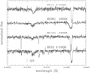 |
Fig. 1 Region of the He I line at 4471 Å and of the Mg II line at 4481 Å for the four stars in NGC 6752. The upper two spectra belong to stars without evidence for diffusion and the lower two show stars with evidence for diffusion. The spectrum of B2281 shows clear signs of rotation, while the situation for B652 is less clear. The offsets in line position indicate deviations of the star’s radial velocity from that of the globular cluster. |
4.3 Identification of observed metal lines
Daospec identifies a line by using the closest wavelength found in the user-provided line catalogue. Because other lines nearby may contribute to a measured line I ran a line identification that selects all lines within ±0.1 Å around the rest wavelength derived by Daospec. If more than one line was found, I inspected the observed line to decide whether this was a true blend and should be excluded from further analysis.
For a start I extracted line lists from the Vienna Atomic Line Database (VALD6, Ryabchikova et al. 2015) for the following combinations of effective temperature, surface gravity, and metallicity [M/H]: for stars affected by diffusion (NGC 6397, NGC 6752) 15 000 K 4.5 +0.5, 20 000 K 4.5 +0.5, 25 000 K 5.0 +0.5; for stars unaffected by diffusion (all clusters) 7000 K 3.0 0.0 (4113), 9157 K 3.07 −0.5 (all others).
Later, I retrieved line lists for the parameters listed in Tables D.1, D.2, D.3, and D.4 to have them tailored to the actual atmospheric parameters. I used microturbulent velocities of 0 km s−1 and requested a minimum line depth of 0.01. For the stars affected by diffusion I used solar metallicity and for the other stars the same metallicities as for the HHe models described earlier. For lines close to each other, I used the information on the predicted depth of the line to decide whether both lines affect the equivalent width. If the predicted depth of one line was less than 5% of that of the other line, I removed the weaker catalogue line and kept the stronger.
In most cases the difference between the observed wavelength of an identified line and the value from the lines list was within ±0.03 Å. For 4113, however, a broad range of offsets was found within ±0.1 Å. Based on the experience with the more reliable spectra of other stars, I restricted the lines used for the abundance analysis of 4113 to those with observed wavelengths within ±0.03 Å of the wavelength from the line list. Doing so provided a good agreement between the abundances derived from Fe I and Fe II lines.
4.4 Abundance analysis
To derive abundances from the equivalent widths I used GALA7 (Mucciarelli et al. 2013). This tool performs an abundance analysis, based on the equivalent widths and grids of model atmospheres. It simultaneously determines the abundances, effective temperature, surface gravities, and microturbulent velocities, together with error estimates. For more details, see Mucciarelli et al. (2013).
I changed the following parameters from the values provided in the tutorial file:
range of valid equivalent widths to cover −9.9 ≤log(Wλ/λ) ≤ −0.1;
error in the equivalent width ≤10% to get robust results;
ion used for optimisation: Fe II for hotter stars.
I found that for the cool blue HB stars in NGC 6397 (T160, T164, T166, and T174) and in NGC 6752 (B944, B2281, B2454, and B2735), which are not affected by radiative levitation, neither abundances, nor their atmospheric parameters could be determined with GALA, because there were too few metal lines. The same applies to the hottest stars in NGC 6752, namely B491, B3699, and B4548, which have either lines from one ionisation stage of iron only or iron lines covering solely a narrow range of excitation energies.
For ions with few lines overall, I reran GALA with an error limit of 15% on the equivalent widths, keeping the effective temperature, surface gravity, and microturbulent velocity fixed to the values determined from equivalent widths with errors of at most 10%.
The abundances for sodium are affected by non-LTE (NLTE) effects as described in Mashonkina et al. (2000). Then, I applied the following corrections to sodium abundances determined for the blue HB stars in NGC 6388: −0.66 (star 1233), −0.39 (star 5235), and -0.36 (star 7788).
The errors for the abundances are derived from the errors of the equivalent widths and the overall scatter of the derived abundance. Abundances are listed only if there are at least two usable lines for the given ion and the abundance uncertainty is below 0.3 dex. GALA may also take into account the uncertainties in effective temperature, surface gravity, and microturbulent velocity; however, this often failed, especially for the surface gravity. Therefore, I ran GALA manually for the atmospheric parameters±uncertainties to get an estimate of these sources of uncertainty. For the stars T179 and T191 in NGC 6397, this procedure did not work because not all necessary models converged. For details and results, we refer to Appendix D.1. The final abundances can be found in Tables D.1, D.2, D.3, and D.4 in Appendix D.2.
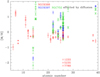 |
Fig. 2 Abundances of stars in NGC 6388 (red symbols) and for stars affected by diffusion in NGC 6397 (blue lozenges) and NGC 6752 (green crosses) relative to the solar abundances of Asplund et al. (2021). |
5 Discussion
5.1 Rotation
The stars B2281 and B652 (possibly) in NGC 6752 show signs rotational broadening in their spectra (see Fig. 1). This is surprising for B652, because the star shows evidence for diffusion, which usually coincides with negligible rotational velocities. The fact that the He I line at 4471 Å is visible in the spectrum of B652 suggests that the diffusion is limited in this star.
5.2 Evidence for pollution in NGC 6388
To verify if the two hotter stars in NGC 6388 (5235 and 7788), which show higher than expected iron abundances, are affected by diffusion I compare in Fig. 2 the abundances of the stars in NGC 6388 to those found for stars affected by diffusion in NGC 6397 and NGC 6752. While the iron and chromium abundances overlap closely, the abundances of silicon, manganese, and yttrium differ substantially, ruling out diffusion as the explanation of the higher iron abundances found for the stars 5235 and (to a lesser extent) 7788 in NGC 6388.
Figure 3 compares for NGC 6388 the abundances from my analysis to those determined for red giant stars in this cluster by Carretta & Bragaglia (2023)8. For most of the elements, the results agree well, with the blue HB stars often showing abundances at the edges of the distribution found by Carretta & Bragaglia (2023). The sodium and oxygen abundances of the HB stars put them at the extreme end of the ‘extreme’ population in Fig. 1 of Carretta & Bragaglia (2023). In addition to the elements covered by Carretta & Bragaglia (2023), the HB stars show low carbon and high nitrogen abundances. Magnesium and aluminium, on the other hand, do not show extreme abundances.
In summary, the observed abundances of carbon, oxygen, nitrogen, and sodium are consistent with the abundance patterns expected for products of hot hydrogen burning, which might produce also helium enrichment. On the other hand, magnesium and aluminium do not show significant differences from the heavy element abundances, so this stronger requirement for helium enrichment has not been satisfied.
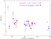 |
Fig. 3 Abundances of stars in NGC 6388 relative to iron from this paper (red open symbols) and from Carretta & Bragaglia (2023) (blue filled squares, adjusted for the different solar abundances used). The error bars for the data from Carretta & Bragaglia (2023) refer to sample errors. |
5.3 Diffusion: Abundance changes with temperature
Figure 4 shows the abundances of silicon, titanium, and iron for the blue HB stars affected by diffusion in NGC 6397, NGC 6752, NGC 288 (Moehler et al. 2014), NGC 1904 (Fabbian et al. 2005), NGC 2808 (Pace et al. 2006), NGC 6205, and NGC 7078 (Behr 2003). For comparison, I also included the abundances of the blue HB stars in NGC 6388 that are unaffected by diffusion.
One obvious common feature are the large star-to-star variations in abundance around the Grundahl jump, namely, at the onset of radiative levitation. The data from Fabbian et al. (2005, open grey circles) tend to follow the data from NGC 288 (Moehler et al. 2014) and NGC 6752. The data from NGC 6205 (open grey triangles) and NGC 7078 (open grey lozenges), both from Behr (2003) instead tend to lie at the lower part of the distribution, while those from NGC 2808 (Pace et al. 2006, open squares) occupy the upper parts of the abundance distribution. For these three clusters, there are no abundances for silicon. NGC 2808 is the most metal-rich cluster for which abundances for hot blue HB stars are available ([M/H] = −1.14, Harris 1996), while NGC 1905 ([M/H] = −1.60, Harris 1996), NGC 6205([M/H] = −1.53, Harris 1996), and NGC 7078 ([M/H] = −2.37, Harris 1996) have similar metallicities to NGC 6752 and NGC 6397. It is unclear how much of the differences may be due to different data and analysis methods.
The different elements shown in Fig. 4 behave differently with effective temperature: titanium shows mainly large scatter without clear trends, possibly due to the fact that it is found only in a subsample of all stars. Silicon shows increasing abundances with higher effective temperatures, which turns into a flat distribution around [Si/H] of about −0.4 (albeit with large scatter) above temperatures of about 13 000 K. Because the silicon data are available only for globular clusters with moderately low metallicities ([M/H] = −1.32… −1.60), it is not clear if the cluster metallicity has any effect.
For iron the scatter at temperatures below about 14 000 K is also large, but caused mostly by the low values for NGC 6205 (open grey triangles). Ignoring those, the abundances increase for effective temperatures of up to 14 000 K and then split into a bimodal distribution, with part of the stars following a trend of decreasing iron abundance with increasing temperature and the other part showing a roughly constant iron abundance of about [Fe/H] = +1 for the same temperature range. It is currently unclear what creates these two branches.
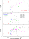 |
Fig. 4 Abundances of silicon, titanium, and iron (relative to the solar abundances of Asplund et al. 2021) vs effective temperature for stars in NGC 6388 (red symbols) and stars affected by diffusion in NGC 288 (magenta asterisks, Moehler et al. 2014), NGC 6397 (blue lozenges), and NGC 6752 (green crosses). The grey symbols mark abundances for HB stars in NGC 1904 (Fabbian et al. 2005), NGC 2808 (Pace et al. 2006), NGC 6205, and NGC 7078 (Behr 2003). |
5.4 Notes to other observers looking for helium enrichment
The high-resolution spectra of cool blue HB stars in metal-rich globular clusters are very well suited to determine metal abundances and atmospheric parameters. For the measurement of helium abundances, on the other hand, a high signal-to-noise ratio and a smooth continuum are more important than having high resolution. This is because the helium lines are inherently broadened and therefore wider and shallower than metal lines.
For cool blue HB stars in metal-poor globular clusters, the situation is quite different because the predicted helium enrichment is generally small and they show very few metal lines. If atmospheric parameters can be determined from other data, medium-resolution spectra with high signal-to-noise are better suited to measure helium abundances for these stars as well, rather than high-resolution spectra with lower signal-to-noise ratios.
Overall, the study of the effects of radiative levitation in the moderately hot HB stars (effective temperatures between about  K and 17 000 K) benefits from high resolution thanks to the many metal lines available, independently of the original metallicity.
6 Conclusions
Blue HB stars in metal-rich globular clusters can provide important constraints on pollution scenarios because they have a high likelihood of being affected by pollution. The results presented here for NGC 6388 may serve as additional constraints when it comes to understanding the status of this exceptional globular cluster. They point towards the presence of products of hot hydrogen-burning in the blue HB stars, which could indicate accompanying helium enrichment; however, the situation is not entirely clear-cut. Additional data (see Sect. 5.4) could help improve the constraints.
The abundances found for silicon, titanium, and iron in moderately hot stars show different trends with effective temperatures, which may indicate the effect of parameters beyond rotation and effective temperature. The question of whether the helium abundance plays a role could be studied in such clusters as NGC 6388 and NGC 6441, for which higher effective temperatures are predicted for the Grundahl jump.
Data availability
The flux calibrated spectra, the measured equivalent widths, and the line parameters used to perform the abundance analyses are available in electronic form at the Strasbourg astronomical Data Centre CDS via anonymous ftp to cdsarc.cds.unistra.fr (130.79.128.5) or via https://cdsarc.cds.unistra.fr/viz-bin/cat/J/A+A/693/A136.
Acknowledgements
The work reported here could not have succeeded without the support of many people. I want to thank them here in the sequence of the time at which they helped me: J. Pritchard for his help in understanding some of the problems I faced with the red arm data, A. Mucciarelli for his patience and support with GALA, S. Villanova for providing me with some testing data of blue HB stars in NGC 6752, E. Pancino for her support in using Daospec and understanding its behaviour, A. Bragaglia and E. Carretta for providing advice about abundances in NGC 6388 and encouragement towards a publication, and, last but by no means least, W.V.D. Dixon, whose referee report improved the content and the readability of this paper immensely. This investigation also could not have been performed without the many services listed below. This research has made use of the NASA’s Astrophysics Data System Bibliographic Services. This work has made use of the VALD database, operated at Uppsala University, the Institute of Astronomy RAS in Moscow, and the University of Vienna (Ryabchikova et al. 2015), and of data from the European Space Agency (ESA) mission Gaia (https://www.cosmos.esa.int/gaia), processed by the Gaia Data Processing and Analysis Consortium (DPAC, https://www.cosmos.esa.int/web/gaia/dpac/consortium). Funding for the DPAC has been provided by national institutions, in particular the institutions participating in the Gaia Multilateral Agreement, and of the VizieR catalogue access tool, CDS, Strasbourg, France. The original description of the VizieR service was published in Ochsenbein et al. (2000). Some of the data presented in this paper were obtained from the Mikulski Archive for Space Telescopes (MAST). STScI is operated by the Association of Universities for Research in Astronomy, Inc., under NASA contract NAS5-26555.
Appendix A Observing information
This section presents the colour–magnitude diagrams of the blue horizontal branches in the three globular clusters, NGC 6388, NGC 6397, and NGC 6752, along with the coordinates, observing times and conditions together with the optical photometric information for the stars discussed in this publication.
A.1 Colour-magnitude diagrams
Here, the colour-magnitude diagrams are shown, based on which the targets have been selected.
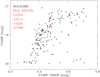 |
Fig. A.1 Colour-magnitude diagram for the globular cluster NGC 6388 using data from the HST UV Globular Cluster Survey (HUGS, Piotto et al. 2015, Nardiello et al. 2018). The red symbols mark the targets of run 69.D-0231(B) |
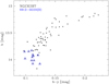 |
Fig. A.2 Colour-magnitude diagram for the globular cluster NGC 6397 using Strömgren photometry from Anthony-Twarog & Twarog (2000). The blue triangles mark the targets of run 69.D-0220(B). |
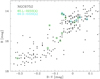 |
Fig. A.3 Colour-magnitude diagram for the globular cluster NGC 6752 using Johnson photometry from Buonanno et al. (1986). The green circles mark the targets of the run 65.L-0233 and the cyan triangles mark the targets of the run 69.D-0220(A). |
A.2 Target and observing information
Here, the coordinates and photometric information for the targets, together with the details of their observations, are listed.
Target coordinates (Gaia Collaboration 2016, 2021) and photometric data (from Piotto et al. 1997) for NGC 6388 together with observing information. The seeing is the average value obtained by the Differential Image Motion Monitor (DIMM), corrected to zenith.
Target coordinates (Gaia Collaboration 2016, 2021) and photometric data for NGC 6397 (Anthony-Twarog & Twarog 2000). The seeing is the average value obtained by the DIMM), corrected to zenith.
Target coordinates (Gaia Collaboration 2016, 2021) and photometric data for NGC 6752 (Buonanno et al. 1986)) together with observing information. The seeing is the average value obtained by the DIMM, corrected to zenith.
Appendix B Observing issues with the data for NGC 6388
Here I describe the problems I encountered with some of the observations obtained for NGC 6388 and how they were solved.
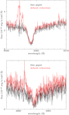 |
Fig. B.1 Top: Hɑ region of the second observation of 5235 from 5 May 2002, reduced as described here (black) and with default reduction parameters (red). One can clearly see the spurious emission on the blue side of the stellar Hɑ line core. Bottom: Hβ region of the observation of 7788 from 12 June 2002, reduced as described here (black) and with default reduction parameters (red). One can clearly see the spurious emission on the blue side of the stellar Hβ line core. |
1233 The data observed for this star on the night starting on 15 June 2002 show a shift of about 100 pixels (comparable to the distance between orders) with respect to the daytime calibrations. Fortunately nighttime calibrations had been observed which could be used to process the data, which showed a shift in wavelength of some 50 Å when reduced with daytime calibrations.
5235 The spectra from 5 May 2002 (start of the night) show blue-shifted emission at Hα (and to a lesser extent at Hβ), which is surprising as cool blue HB stars are not known for emission lines. A closer inspection revealed that the orders of the spectrum had shifted between the science observations and the corresponding daytime calibrations, which caused an imperfect sky subtraction and retained background Hα emission in the extracted spectrum. By using the science spectra to identify the order centre and reducing the slit length for the spectrum extraction to 20 pixels this problem could be solved (see Fig. B.1, top).
7788 Despite the attempts to select isolated targets a faint additional spectrum appears in the slit for the red arm. To avoid contamination by this additional source this the slit length was again reduced to 20 pixels. In addition the data observed for this star on 11, 12, and 13 June 2002 (start of the night) suffer again from order shifts between science data and daytime calibrations, which cause spurious emission in the line cores of Hα and Hβ. This problem could be solved for the data from June 11 and 12 by using the science spectra to identify the order centre (see Fig. B.1, bottom). The shift of the science data from June 13 was too large to recover the red part of the red arm.
Appendix C Atmospheric parameters derived from line profile fitting
Here, I provide the results of the line profile fitting process described in Sect. 3.
Atmospheric parameters for the stars in NGC 6397 (T<number>) and NGC 6752 (B<number>) from fitting the hydrogen and (if available) helium line profiles for stars without evidence of diffusion. The values in italics are taken from Moehler et al. (2000, Table 1).
Atmospheric parameters for the stars affected by diffusion in NGC 6397 and NGC 6752 from fitting the hydrogen and (if available) helium line profiles and from the GALA analysis. The values in italics are taken from Moehler et al. (2000, Table 2).
Appendix D Results of the abundance analysis
D.1 Uncertainties
To determine uncertainties in the abundances caused by uncertainties in the atmospheric parameter, I used the uncertainties listed below. The resulting offsets in abundances are shown in Fig. D.1.
For NGC 6388 I used the effective temperature and surface gravity estimates marked in bold font in Table 2 as starting values. The atmospheric parameters and abundances resulting from the GALA analysis are listed in Table D.1. I used uncertainties in effective temperature as follows: 50 K for 1233, 250 K for 4113, 120K for 5235, and 150 K for 7788. For the surface gravity I used an uncertainty of 0.1 dex for all stars except 4113 (0.2 dex).
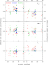 |
Fig. D.1 Offsets in abundances determined by applying the estimated uncertainties (one at a time) for effective temperature (top row), surface gravity (middle row), and microturbulent velocity (bottom row) to the corresponding parameters determined by GALA and then rerunning GALA with fixed parameters. The left column shows the effect of subtracting the uncertainties, the right one the effect of adding the uncertainties. Red open symbols (circle, square, triangle) mark the stars in NGC 6388, blue lozenges the ones in NGC 6397, and green crosses the ones in NGC 6752. |
For the stars in NGC 6397 and NGC 6752, I used the atmospheric parameters derived from spectral line fitting as starting values. The results of the GALA analysis are listed in Tables D.2, D.3 (both for NGC 6752), and D.4 (NGC 6397). For stars in NGC 6752 and NGC 6397 observed with program 69.D-0220 I used an uncertainty of 90 K in effective temperature and of 0.04 dex in surface gravity. For the hotter stars in NGC 6752 observed with program 65.L-0233 I used uncertainties of 210 K and 0.1 dex in effective temperature and surface gravity, respectively. For all stars, I used an uncertainty of 0.2 km s−1 for the microturbulence.
D.2 Abundances
In this section, I list the abundances for the blue HB stars in NGC 6388; (Table D.1), NGC 6397 (Table D.4), and NGC 6752 (Tables D.2 and D.3) derived as described in Sect. 4.
Chemical abundances derived for NGC 6388 stars with GALA using the atmospheric parameters derived from the HUGS photometry (Table 2) as starting values. Values in italics were obtained with errors of 15% of the equivalent width. The references for the line parameters used for the analysis can be found in Table E.1..
Chemical abundances derived for NGC 6752 stars (65.L-0233(A)) with GALA using atmospheric parameters from spectral line profile fitting (Table C.2) as starting values. Values in italics were obtained with errors of 15% of the equivalent width. The references for the line parameters used for the analysis can be found in Tables E.1 and E.2.
Appendix E References for VALD line lists
In addition to the references listed below the following publications have been used for isotopic scaling: Nouri et al. (2010, Ti II), Mårtensson-Pendrill et al. (1992, Ca II), Kurucz (2008, Ni I). In 2012 T. A. Ryabchikova determined averaged transition probabilities 919 for Si II lines using the data from Schulz-Gulde (1969), Blanco et al. (1995), and Matheron et al. (2001). These averaged values are available only in the VALD (bibcode Si2-av1) and I have used them for stars in all three globular clusters.
References for the lines lists obtained from VALD for the abundance analysis of the stars in NGC 6397 and NGC 6752.
This table provides the references for the lines lists obtained from VALD for the abundance analysis of the stars in NGC 6388.
References
- Aldenius, M., Tanner, J. D., Johansson, S., Lundberg, H., & Ryan, S. G. 2007, A&A, 461, 767 [NASA ADS] [CrossRef] [EDP Sciences] [Google Scholar]
- Anderson, E. M., Zilitis, V. A., & Sorokina, E. S. 1967, Opt. Spectrosc., 23, 102 [NASA ADS] [Google Scholar]
- Anthony-Twarog, B. J., & Twarog, B. A. 2000, AJ, 120, 3111 [Google Scholar]
- Asplund, M., Amarsi, A. M., & Grevesse, N. 2021, A&A, 653, A141 [NASA ADS] [CrossRef] [EDP Sciences] [Google Scholar]
- Bard, A., & Kock, M. 1994, A&A, 282, 1014 [NASA ADS] [Google Scholar]
- Bard, A., Kock, A., & Kock, M. 1991, A&A, 248, 315 [NASA ADS] [Google Scholar]
- Barklem, P. S., & Aspelund-Johansson, J. 2005, A&A, 435, 373 [NASA ADS] [CrossRef] [EDP Sciences] [Google Scholar]
- Barklem, P. S., Piskunov, N., & O’Mara, B. J. 2000, A&AS, 142, 467 [NASA ADS] [CrossRef] [EDP Sciences] [Google Scholar]
- Baschek, B., Garz, T., Holweger, H., & Richter, J. 1970, A&A, 4, 229 [NASA ADS] [Google Scholar]
- Bastian, N., & Lardo, C. 2018, ARA&A, 56, 83 [Google Scholar]
- Bedin, L. R., Piotto, G., Anderson, J., et al. 2004, ApJ, 605, L125 [Google Scholar]
- Behr, B. B. 2003, ApJS, 149, 67 [NASA ADS] [CrossRef] [Google Scholar]
- Behr, B. B., Cohen, J. G., McCarthy, J. K., & Djorgovski, S. G. 1999, ApJ, 517, L135 [NASA ADS] [CrossRef] [Google Scholar]
- Behr, B. B., Cohen, J. G., & McCarthy, J. K. 2000, ApJ, 531, L37 [NASA ADS] [CrossRef] [Google Scholar]
- Bergeron, P., Saffer, R. A., & Liebert, J. 1992, ApJ, 394, 228 [NASA ADS] [CrossRef] [Google Scholar]
- Blackwell, D. E., Shallis, M. J., & Simmons, G. J. 1980, A&A, 81, 340 [NASA ADS] [Google Scholar]
- Blanco, F., Botho, B., & Campos, J. 1995, Phys. Scr, 52, 628 [Google Scholar]
- Bohlin, R. C., Gordon, K. D., & Tremblay, P.-E. 2014, PASP, 126, 711 [Google Scholar]
- Bohlin, R. C., Hubeny, I., & Rauch, T. 2020, AJ, 160, 21 [Google Scholar]
- Bridges, J. M. 1973, in Phenomena in Ionized Gases, Eleventh International Conference, ed. I. Štoll, 418 [Google Scholar]
- Brown, T. M., Cassisi, S., D’Antona, F., et al. 2016, ApJ, 822, 44 [NASA ADS] [CrossRef] [Google Scholar]
- Buonanno, R., Caloi, V., Castellani, V., et al. 1986, A&AS, 66, 79 [NASA ADS] [Google Scholar]
- Busso, G., Cassisi, S., Piotto, G., et al. 2007, A&A, 474, 105 [NASA ADS] [CrossRef] [EDP Sciences] [Google Scholar]
- Carretta, E., & Bragaglia, A. 2022, A&A, 659, A122 [NASA ADS] [CrossRef] [EDP Sciences] [Google Scholar]
- Carretta, E., & Bragaglia, A. 2023, A&A, 677, A73 [NASA ADS] [CrossRef] [EDP Sciences] [Google Scholar]
- Corliss, C. H., & Bozman, W. R. 1962, NBS Monograph, 53, Experimental Transition Probabilities for Spectral Lines of Seventy Elements; derived from the NBS Tables of Spectral-line intensities, eds. C. H. Corliss, & W. R. Bozman (US Government Printing Office) [CrossRef] [Google Scholar]
- Crocker, D. A., Rood, R. T., & O’Connell, R. W. 1988, ApJ, 332, 236 [NASA ADS] [CrossRef] [Google Scholar]
- Den Hartog, E. A., Lawler, J. E., Sobeck, J. S., Sneden, C., & Cowan, J. J. 2011, ApJS, 194, 35 [NASA ADS] [CrossRef] [Google Scholar]
- Fabbian, D., Recio-Blanco, A., Gratton, R. G., & Piotto, G. 2005, A&A, 434, 235 [NASA ADS] [CrossRef] [EDP Sciences] [Google Scholar]
- Fitzpatrick, E. L., Massa, D., Gordon, K. D., Bohlin, R., & Clayton, G. C. 2019, ApJ, 886, 108 [Google Scholar]
- Freudling, W., Romaniello, M., Bramich, D. M., et al. 2013, A&A, 559, A96 [NASA ADS] [CrossRef] [EDP Sciences] [Google Scholar]
- Fuhr, J. R., Martin, G. A., & Wiese, W. L. 1988, Journal of Physical and Chemical Reference Data, 17, Suppl. 4. (New York: American Institute of Physics (AIP) and American Chemical Society), 17 [NASA ADS] [Google Scholar]
- Gaia Collaboration (Prusti, T., et al.) 2016, A&A, 595, A1 [NASA ADS] [CrossRef] [EDP Sciences] [Google Scholar]
- Gaia Collaboration (Brown, A. G. A., et al.) 2021, A&A, 649, A1 [NASA ADS] [CrossRef] [EDP Sciences] [Google Scholar]
- Gratton, R. G., Carretta, E., Bragaglia, A., Lucatello, S., & D’Orazi, V. 2010, A&A, 517, A81 [CrossRef] [EDP Sciences] [Google Scholar]
- Grundahl, F., Catelan, M., Landsman, W. B., Stetson, P. B., & Andersen, M. I. 1999, ApJ, 524, 242 [NASA ADS] [CrossRef] [Google Scholar]
- Hannaford, P., Lowe, R. M., Grevesse, N., Biemont, E., & Whaling, W. 1982, ApJ, 261, 736 [NASA ADS] [CrossRef] [Google Scholar]
- Hannaford, P., Lowe, R. M., Grevesse, N., & Noels, A. 1992, A&A, 259, 301 [NASA ADS] [Google Scholar]
- Harris, W. E. 1996, AJ, 112, 1487 [Google Scholar]
- Hui-Bon-Hoa, A., LeBlanc, F., & Hauschildt, P. H. 2000, ApJ, 535, L43 [NASA ADS] [CrossRef] [Google Scholar]
- Husser, T.-O., Kamann, S., Dreizler, S., et al. 2016, A&A, 588, A148 [NASA ADS] [CrossRef] [EDP Sciences] [Google Scholar]
- Kling, R., Schnabel, R., & Griesmann, U. 2001, ApJS, 134, 173 [NASA ADS] [CrossRef] [Google Scholar]
- Kramida, A., Ralchenko, Y., Reader, J., & NIST ASD Team 2022, NIST Atomic Spectra Database (ver. 5.10) [Google Scholar]
- Kroll, S., & Kock, M. 1987, A&AS, 67, 225 [NASA ADS] [Google Scholar]
- Kurucz, R. L. 2003, Robert L. Kurucz on-line database of observed and predicted atomic transitions, http://kurucz.harvard.edu/atoms/ [Google Scholar]
- Kurucz, R. L. 2007, Robert L. Kurucz on-line database of observed and predicted atomic transitions, http://kurucz.harvard.edu/atoms/ [Google Scholar]
- Kurucz, R. L. 2008, Robert L. Kurucz on-line database of observed and predicted atomic transitions, http://kurucz.harvard.edu/atoms/ [Google Scholar]
- Kurucz, R. L. 2009, Robert L. Kurucz on-line database of observed and predicted atomic transitions, http://kurucz.harvard.edu/atoms/ [Google Scholar]
- Kurucz, R. L. 2010, Robert L. Kurucz on-line database of observed and predicted atomic transitions, http://kurucz.harvard.edu/atoms/ [Google Scholar]
- Kurucz, R. L. 2011, Robert L. Kurucz on-line database of observed and predicted atomic transitions, http://kurucz.harvard.edu/atoms/ [Google Scholar]
- Kurucz, R. L. 2012, Robert L. Kurucz on-line database of observed and predicted atomic transitions, http://kurucz.harvard.edu/atoms/ [Google Scholar]
- Kurucz, R. L. 2013, Robert L. Kurucz on-line database of observed and predicted atomic transitions, http://kurucz.harvard.edu/atoms/ [Google Scholar]
- Kurucz, R. L. 2014, Robert L. Kurucz on-line database of observed and predicted atomic transitions, http://kurucz.harvard.edu/atoms/ [Google Scholar]
- Kurucz, R. L. 2016, Robert L. Kurucz on-line database of observed and predicted atomic transitions, http://kurucz.harvard.edu/atoms/ [Google Scholar]
- Kurucz, R. L. 2017, Robert L. Kurucz on-line database of observed and predicted atomic transitions, http://kurucz.harvard.edu/atoms/ [Google Scholar]
- Kurucz, R. L., & Peytremann, E. 1975, SAO Spec. Rep., 362, 1 [NASA ADS] [Google Scholar]
- Lardo, C., Pancino, E., Bellazzini, M., et al. 2015, A&A, 573, A115 [NASA ADS] [CrossRef] [EDP Sciences] [Google Scholar]
- Lawler, J. E., Bonvallet, G., & Sneden, C. 2001, ApJ, 556, 452 [NASA ADS] [CrossRef] [Google Scholar]
- Lawler, J. E., Sneden, C., Nave, G., et al. 2017, ApJS, 228, 10 [CrossRef] [Google Scholar]
- Lawler, J. E., Hala, Sneden, C., et al. 2019, ApJS, 241, 21 [NASA ADS] [CrossRef] [Google Scholar]
- LeBlanc, F., Monin, D., Hui-Bon-Hoa, A., & Hauschildt, P. H. 2009, A&A, 495, 937 [NASA ADS] [CrossRef] [EDP Sciences] [Google Scholar]
- Lee, Y.-W., Joo, S.-J., Han, S.-I., et al. 2005, ApJ, 621, L57 [NASA ADS] [CrossRef] [Google Scholar]
- Lincke, R., & Ziegenbein, B. 1971, Z. Phys., 241, 369 [NASA ADS] [CrossRef] [Google Scholar]
- Litzèn, U., Brault, J. W., & Thorne, A. P. 1993, Phys. Scr, 47, 628 [CrossRef] [Google Scholar]
- Mårtensson-Pendrill, A.-M., Ynnerman, A., Warston, H., et al. 1992, Phys. Rev. A, 45, 4675 [CrossRef] [Google Scholar]
- Mashonkina, L. I., Shimanskii, V. V., & Sakhibullin, N. A. 2000, Astron. Rep., 44, 790 [NASA ADS] [CrossRef] [Google Scholar]
- Matheron, P., Escarguel, A., Redon, R., Lesage, A., & Richou, J. 2001, J. Quant. Spec. Radiat. Transf., 69, 535 [NASA ADS] [CrossRef] [Google Scholar]
- Milone, A. P., Marino, A. F., Dotter, A., et al. 2014, ApJ, 785, 21 [NASA ADS] [CrossRef] [Google Scholar]
- Moehler, S., & Sweigart, A. V. 2006, A&A, 455, 943 [NASA ADS] [CrossRef] [EDP Sciences] [Google Scholar]
- Moehler, S., Heber, U., & de Boer, K. S. 1995, A&A, 294, 65 [NASA ADS] [Google Scholar]
- Moehler, S., Heber, U., & Rupprecht, G. 1997, A&A, 319, 109 [NASA ADS] [Google Scholar]
- Moehler, S., Sweigart, A. V., Landsman, W. B., & Heber, U. 2000, A&A, 360, 120 [NASA ADS] [Google Scholar]
- Moehler, S., Dreizler, S., LeBlanc, F., et al. 2014, A&A, 565, A100 [NASA ADS] [CrossRef] [EDP Sciences] [Google Scholar]
- Mucciarelli, A., Pancino, E., Lovisi, L., Ferraro, F. R., & Lapenna, E. 2013, ApJ, 766, 78 [NASA ADS] [CrossRef] [Google Scholar]
- Napiwotzki, R., Green, P. J., & Saffer, R. A. 1999, ApJ, 517, 399 [NASA ADS] [CrossRef] [Google Scholar]
- Nardiello, D., Libralato, M., Piotto, G., et al. 2018, MNRAS, 481, 3382 [NASA ADS] [CrossRef] [Google Scholar]
- Norris, J. E. 2004, ApJ, 612, L25 [NASA ADS] [CrossRef] [Google Scholar]
- Nouri, Z., Rosner, S. D., Li, R., Scholl, T. J., & Holt, R. A. 2010, Phys. Scr, 81, 065301 [Google Scholar]
- O’Brian, T. R., Wickliffe, M. E., Lawler, J. E., Whaling, W., & Brault, J. W. 1991, J. Opt. Soc. Am. B Opt. Phys., 8, 1185 [Google Scholar]
- Ochsenbein, F., Bauer, P., & Marcout, J. 2000, A&AS, 143, 23 [NASA ADS] [CrossRef] [EDP Sciences] [Google Scholar]
- Pace, G., Recio-Blanco, A., Piotto, G., & Momany, Y. 2006, A&A, 452, 493 [NASA ADS] [CrossRef] [EDP Sciences] [Google Scholar]
- Pauls, U., Grevesse, N., & Huber, M. C. E. 1990, A&A, 231, 536 [NASA ADS] [Google Scholar]
- Pickering, J. C., Thorne, A. P., & Perez, R. 2001, ApJS, 132, 403 [Google Scholar]
- Piotto, G., Sosin, C., King, I. R., et al. 1997, in Stellar Ecology: Advances in Stellar Evolution, 84 [Google Scholar]
- Piotto, G., Villanova, S., Bedin, L. R., et al. 2005, ApJ, 621, 777 [Google Scholar]
- Piotto, G., Milone, A. P., Bedin, L. R., et al. 2015, AJ, 149, 91 [Google Scholar]
- Raassen, A. J. J., & Uylings, P. H. M. 1998, A&A, 340, 300 [Google Scholar]
- Ralchenko, Y., Kramida, A., Reader, J., & NIST ASD Team 2010, NIST Atomic Spectra Database (ver. 4.0.0) [Google Scholar]
- Rich, R. M., Sosin, C., Djorgovski, S. G., et al. 1997, ApJ, 484, L25 [NASA ADS] [CrossRef] [Google Scholar]
- Ryabchikova, T. A., Hill, G. M., Landstreet, J. D., Piskunov, N., & Sigut, T. A. A. 1994, MNRAS, 267, 697 [NASA ADS] [CrossRef] [Google Scholar]
- Ryabchikova, T. A., Piskunov, N. E., Stempels, H. C., Kupka, F., & Weiss, W. W. 1999, Phys. Scr. Vol. T, 83, 162 [Google Scholar]
- Ryabchikova, T., Piskunov, N., Kurucz, R. L., et al. 2015, Phys. Scr, 90, 054005 [Google Scholar]
- Saffer, R. A., Bergeron, P., Koester, D., & Liebert, J. 1994, ApJ, 432, 351 [NASA ADS] [CrossRef] [Google Scholar]
- Saloman, E. B. 2012, J. Phys. Chem. Ref. Data, 41, 013101 [NASA ADS] [CrossRef] [Google Scholar]
- Sandage, A., & Wildey, R. 1967, ApJ, 150, 469 [NASA ADS] [CrossRef] [Google Scholar]
- Sansonetti, C. J., & Nave, G. 2014, ApJS, 213, 28 [NASA ADS] [CrossRef] [Google Scholar]
- Schulz-Gulde, E. 1969, J. Quant. Spec. Radiat. Transf., 9, 13 [NASA ADS] [CrossRef] [Google Scholar]
- Seaton, M. J., Yan, Y., Mihalas, D., & Pradhan, A. K. 1994, MNRAS, 266, 805 [NASA ADS] [CrossRef] [Google Scholar]
- Smith, G. 1988, J. Phys. B At. Mol. Phys., 21, 2827 [NASA ADS] [CrossRef] [Google Scholar]
- Smith, W. W., & Gallagher, A. 1966, Phys. Rev., 145, 26 [NASA ADS] [CrossRef] [Google Scholar]
- Smith, W. H., & Liszt, H. S. 1971, J. Opt. Soc. Am., 61, 938 [NASA ADS] [CrossRef] [Google Scholar]
- Smith, G., & O’Neill, J. A. 1975, A&A, 38, 1 [NASA ADS] [Google Scholar]
- Smith, G., & Raggett, D. S. J. 1981, J. Phys. B At. Mol. Phys., 14, 4015 [NASA ADS] [CrossRef] [Google Scholar]
- Sobeck, J. S., Lawler, J. E., & Sneden, C. 2007, ApJ, 667, 1267 [NASA ADS] [CrossRef] [Google Scholar]
- Stetson, P. B., & Pancino, E. 2008, PASP, 120, 1332 [Google Scholar]
- Sugar, J., & Corliss, C. 1985, Atomic Energy Levels of the Iron-period Elements: Potassium through Nickel (Washington: American Chemical Society) [Google Scholar]
- ten Bruggencate, P. 1927, Sternhaufen (Berlin: Springer) [CrossRef] [Google Scholar]
- Theodosiou, C. E. 1989, Phys. Rev. A, 39, 4880 [NASA ADS] [CrossRef] [Google Scholar]
- Thorne, A. P., Pickering, J. C., & Semeniuk, J. I. 2013, ApJS, 207, 13 [NASA ADS] [CrossRef] [Google Scholar]
- Vaca, R. J., Cabrera-Ziri, I., Magris, G. C., Bastian, N., & Salaris, M. 2024, A&A, 690, A199 [NASA ADS] [CrossRef] [EDP Sciences] [Google Scholar]
- van den Bergh, S. 1967, AJ, 72, 70 [NASA ADS] [CrossRef] [Google Scholar]
- Vasiliev, E., & Baumgardt, H. 2021, MNRAS, 505, 5978 [NASA ADS] [CrossRef] [Google Scholar]
- Villanova, S., Piotto, G., & Gratton, R. G. 2009, A&A, 499, 755 [NASA ADS] [CrossRef] [EDP Sciences] [Google Scholar]
- Wiese, W. L., Smith, M. W., & Glennon, B. M. 1966, Atomic Transition Probabilities: Hydrogen through Neon. A Critical Data Compilation, eds. W. L. Wiese, M. W. Smith, & B. M. Glennon, (US Government Printing Office) [Google Scholar]
- Wood, M. P., Lawler, J. E., Sneden, C., & Cowan, J. J. 2013, ApJS, 208, 27 [NASA ADS] [CrossRef] [Google Scholar]
- Wood, M. P., Lawler, J. E., Den Hartog, E. A., Sneden, C., & Cowan, J. J. 2014a, ApJS, 214, 18 [Google Scholar]
- Wood, M. P., Lawler, J. E., Sneden, C., & Cowan, J. J. 2014b, ApJS, 211, 20 [NASA ADS] [CrossRef] [Google Scholar]
I use the solar abundances from Asplund et al. (2021), which differ slightly from those used by Carretta & Bragaglia (2023). When comparing my abundances to those of Carretta & Bragaglia (2023) I adjust for those differences.
All Tables
Photometric data and membership probabilities for the target stars in NGC 6388 from the HUGS survey (Piotto et al. 2015, Nardiello et al. 2018), derived with Method1.
Effective temperature and surface gravity estimates for the HB stars in NGC 6388 obtained from HUGS (Piotto et al. 2015, Nardiello et al. 2018) data, using Kurucz model spectra for [M/H] = –0.5.
Target coordinates (Gaia Collaboration 2016, 2021) and photometric data (from Piotto et al. 1997) for NGC 6388 together with observing information. The seeing is the average value obtained by the Differential Image Motion Monitor (DIMM), corrected to zenith.
Target coordinates (Gaia Collaboration 2016, 2021) and photometric data for NGC 6397 (Anthony-Twarog & Twarog 2000). The seeing is the average value obtained by the DIMM), corrected to zenith.
Target coordinates (Gaia Collaboration 2016, 2021) and photometric data for NGC 6752 (Buonanno et al. 1986)) together with observing information. The seeing is the average value obtained by the DIMM, corrected to zenith.
Atmospheric parameters for the stars in NGC 6397 (T<number>) and NGC 6752 (B<number>) from fitting the hydrogen and (if available) helium line profiles for stars without evidence of diffusion. The values in italics are taken from Moehler et al. (2000, Table 1).
Atmospheric parameters for the stars affected by diffusion in NGC 6397 and NGC 6752 from fitting the hydrogen and (if available) helium line profiles and from the GALA analysis. The values in italics are taken from Moehler et al. (2000, Table 2).
Chemical abundances derived for NGC 6388 stars with GALA using the atmospheric parameters derived from the HUGS photometry (Table 2) as starting values. Values in italics were obtained with errors of 15% of the equivalent width. The references for the line parameters used for the analysis can be found in Table E.1..
Chemical abundances derived for NGC 6752 stars (65.L-0233(A)) with GALA using atmospheric parameters from spectral line profile fitting (Table C.2) as starting values. Values in italics were obtained with errors of 15% of the equivalent width. The references for the line parameters used for the analysis can be found in Tables E.1 and E.2.
References for the lines lists obtained from VALD for the abundance analysis of the stars in NGC 6397 and NGC 6752.
This table provides the references for the lines lists obtained from VALD for the abundance analysis of the stars in NGC 6388.
All Figures
|
Fig. 1 Region of the He I line at 4471 Å and of the Mg II line at 4481 Å for the four stars in NGC 6752. The upper two spectra belong to stars without evidence for diffusion and the lower two show stars with evidence for diffusion. The spectrum of B2281 shows clear signs of rotation, while the situation for B652 is less clear. The offsets in line position indicate deviations of the star’s radial velocity from that of the globular cluster. |
| In the text | |
|
Fig. 2 Abundances of stars in NGC 6388 (red symbols) and for stars affected by diffusion in NGC 6397 (blue lozenges) and NGC 6752 (green crosses) relative to the solar abundances of Asplund et al. (2021). |
| In the text | |
|
Fig. 3 Abundances of stars in NGC 6388 relative to iron from this paper (red open symbols) and from Carretta & Bragaglia (2023) (blue filled squares, adjusted for the different solar abundances used). The error bars for the data from Carretta & Bragaglia (2023) refer to sample errors. |
| In the text | |
|
Fig. 4 Abundances of silicon, titanium, and iron (relative to the solar abundances of Asplund et al. 2021) vs effective temperature for stars in NGC 6388 (red symbols) and stars affected by diffusion in NGC 288 (magenta asterisks, Moehler et al. 2014), NGC 6397 (blue lozenges), and NGC 6752 (green crosses). The grey symbols mark abundances for HB stars in NGC 1904 (Fabbian et al. 2005), NGC 2808 (Pace et al. 2006), NGC 6205, and NGC 7078 (Behr 2003). |
| In the text | |
|
Fig. A.1 Colour-magnitude diagram for the globular cluster NGC 6388 using data from the HST UV Globular Cluster Survey (HUGS, Piotto et al. 2015, Nardiello et al. 2018). The red symbols mark the targets of run 69.D-0231(B) |
| In the text | |
|
Fig. A.2 Colour-magnitude diagram for the globular cluster NGC 6397 using Strömgren photometry from Anthony-Twarog & Twarog (2000). The blue triangles mark the targets of run 69.D-0220(B). |
| In the text | |
|
Fig. A.3 Colour-magnitude diagram for the globular cluster NGC 6752 using Johnson photometry from Buonanno et al. (1986). The green circles mark the targets of the run 65.L-0233 and the cyan triangles mark the targets of the run 69.D-0220(A). |
| In the text | |
|
Fig. B.1 Top: Hɑ region of the second observation of 5235 from 5 May 2002, reduced as described here (black) and with default reduction parameters (red). One can clearly see the spurious emission on the blue side of the stellar Hɑ line core. Bottom: Hβ region of the observation of 7788 from 12 June 2002, reduced as described here (black) and with default reduction parameters (red). One can clearly see the spurious emission on the blue side of the stellar Hβ line core. |
| In the text | |
|
Fig. D.1 Offsets in abundances determined by applying the estimated uncertainties (one at a time) for effective temperature (top row), surface gravity (middle row), and microturbulent velocity (bottom row) to the corresponding parameters determined by GALA and then rerunning GALA with fixed parameters. The left column shows the effect of subtracting the uncertainties, the right one the effect of adding the uncertainties. Red open symbols (circle, square, triangle) mark the stars in NGC 6388, blue lozenges the ones in NGC 6397, and green crosses the ones in NGC 6752. |
| In the text | |
Current usage metrics show cumulative count of Article Views (full-text article views including HTML views, PDF and ePub downloads, according to the available data) and Abstracts Views on Vision4Press platform.
Data correspond to usage on the plateform after 2015. The current usage metrics is available 48-96 hours after online publication and is updated daily on week days.
Initial download of the metrics may take a while.