| Issue |
A&A
Volume 693, January 2025
|
|
|---|---|---|
| Article Number | L8 | |
| Number of page(s) | 7 | |
| Section | Letters to the Editor | |
| DOI | https://doi.org/10.1051/0004-6361/202452408 | |
| Published online | 06 January 2025 | |
Letter to the Editor
The density profile of Milky Way dark matter halo constrained from the OGLE microlensing sky map
1
Department of Astronomy, School of Physical Science, University of Science and Technology of China, Hefei, Anhui 230026, China
2
Institute of Deep Space Sciences, Deep Space Exploration Laboratory, Hefei 230026, China
3
School of Physics and Astronomy, Sun Yat-sen University, 2 Daxue Road, Zhuhai 519082, China
4
Department of Physics and Astronomy, University of Utah, Salt Lake City, UT 84102, USA
5
Department of Astronomy, University of Michigan, 1085 S. University, Ann Arbor, MI 48109, USA
⋆ Corresponding authors; This email address is being protected from spambots. You need JavaScript enabled to view it.
, This email address is being protected from spambots. You need JavaScript enabled to view it.
Received:
29
September
2024
Accepted:
21
November
2024
Abstract
We report the detection of a core with a size of 282−31+34 pc in the center of Milky Way dark matter halo at the 68% confidence level. It was detected using the microlensing event-rate sky map data from the optical gravitational lensing experiment (OGLE) survey. We applied the spatial information of the microlensing sky map and modeled it with the detailed Milky Way dark matter halo core-cusp profile, and with the fraction of dark matter in the form of mini dark matter structure (MDMS; fMDMS = ΩMDMS/ΩDM) such as a primordial black hole, Earth-mass subhalos, or floating planets. This sky map can simultaneously constrain fMDMS and the core size without a strong degeneracy while fully considering the mass function of Milky Way stellar components from the bulge and disk.
Key words: Galaxy: halo / dark matter
© The Authors 2025
 Open Access article, published by EDP Sciences, under the terms of the Creative Commons Attribution License (https://creativecommons.org/licenses/by/4.0), which permits unrestricted use, distribution, and reproduction in any medium, provided the original work is properly cited.
This article is published in open access under the Subscribe to Open model. This email address is being protected from spambots. You need JavaScript enabled to view it. to support open access publication.
1. Introduction
The concordance cosmology is a successful model. That fits most of the observations with only half a dozen parameters, such as the cosmic microwave background (CMB) (Planck Collaboration VI 2020), supernova Ia (SNIa) (Riess et al. 1998), time-delay projects based on strongly lensed active galactic nuclei (AGNs) (Birrer et al. 2020), and weak-lensing statistics (Hikage et al. 2019). However, despite all these successes, differences emerge among different cosmological probes, for example, the recent Hubble tension between Planck observation and SNIa (Verde et al. 2019), or the “lensing is low” issue on cosmological parameters between weak-lensing measurements and CMB (Leauthaud et al. 2017).
On small scales, there are also a series of crises. These include the missing satellite problem (MSP), too big to fail (TBTF), and the core-cusp problem (CCP) (de Blok 2010). Especially the core-cusp problem, which describes the situation that the inferred dark-matter core structure from nearby dwarf galaxies contradicts the Navarro-Frenk-White (NFW) profile, the cuspy profile from pure cold dark-matter simulations (Navarro et al. 1997) caused extensive studies of the formation mechanism of the core structure. This was done either with an exotic self-interacting dark matter model (SIDM) (Spergel & Steinhardt 2000; Jiang et al. 2023) or with an astrophysical model from baryonic feedback and merging, dynamical friction, and so on (see the review papers of Salucci 2019; Del Popolo & Le Delliou 2022). Moreover, the enigmatic Gould belt might be created by a dark matter core that collides with the gas disk of the Milky Way (Diemand et al. 2008; Bekki 2009). However, there is no conclusive observational evidence so far to either confirm or reject the aforementioned core structure of Milky Way, largely because dark matter itself cannot be directly observed and because the rotation curve of Milky Way is not as informative as that of nearby dwarf galaxies (Gentile et al. 2004; Bekki 2009; Karukes & Salucci 2017). New probes are therefore necessary to map the dark side of the Milky Way, and these maps then need to be compared to simulations. This will boost our understanding of the core formation of the Milky Way halo and related problems.
The method we develop here is based on the assumption that a fraction of the dark matter is in the form of primordial black holes (Novikov et al. 1979; Carr & Kühnel 2020; Sasaki et al. 2018), or in the form of mini dark matter halos with hundreds of Earth masses (Wang et al. 2020), which is similar to the so-called dark matter minihalos (Delos & Silk 2023) with internal density of 1012 M⊙/pc3. We generalized these as mini dark matter structures (MDMS) that follow the density profile of the Milky Way dark matter halo and can induce a microlensing event when they intersect the line between the background star and the observer.
Fig. 1 presents the patterns of the microlensing event-rate sky map for the cuspy NFW profile (left panel) and the core-density profile (middle panel). The right panel shows the event-rate sky map of the newest OGLE data release (Mróz et al. 2019). By fitting the OGLE sky map, we can constrain the dark matter density profile.
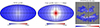 |
Fig. 1. Sky maps in a Mollweide projection. Left panel: Microlensing event rate in an NFW density profile. Middle panel: Event rate for a core of 282 pc. Right panel: sky map of 5790 OGLE microlensing events. The difference between the graticules are 2 deg in longitude and 4.5 deg in latitude. As we are unable to reach all the detailed data of the microlensing events that were used to build the catalog, we cannot plot an event-rate sky map (see Fig. 24 of Mróz et al. 2020). |
We serendipitously found that the spatial distribution of the microlensing event-rate sky map targeting the Galactic center from Optical Gravitational Lensing Experiment (OGLE) (Mróz et al. 2020) can simultaneoulsy place strong constraints on the fraction of mini dark matter structures (MDMS) and on the core size of the central part of the Milky Way dark matter halo. The inferred size of the dark core is 282 pc at the 68% confidence level. Furthermore, this result can place constraints on dark matter models beyond the cold dark matter (CDM) or the baryonic physics of the Milky Way (Wetzel et al. 2023). Either way, this discovery opens another window into the mystery of the core-cusp problem.
2. Microlensing model
Our model extends the microlensing geometry and notations in (Niikura et al. 2019) by fully employing the spatial information. We took the x-direction to be along the line connecting the Galactic center and the Earth (the observer’s position), with the assumption that the Earth is located at (x, y, z) = (8 kpc, 0, 0). The y-direction was the rotating direction of the Earth in the Galactic disk plane, and the z-direction was perpendicular to the plane.
We denote the mass of the lens as M, and the source-observer, lens-observer, and source-lens distance are denoted ds, dl, and dls = ds − dl. In our coordinate system, a lens at dl is located at x = 8kpc − dl cos l cos b, y = dl cos b sin l, and z = dl sin b. As the OGLE survey mainly focuses on the source near the Galactic center, we assumed ds = 8 kpc for all the sources, as was done in Niikura et al. (2019). With the above notation, the Einstein radius RE for a given mass M can be expressed as
 (1)
(1)
For simplicity, we considered that all the lenses had an identical mass of M for MDMS, but a stellar mass function (see the following section) for the bulge and disk contribution. They both followed the Maxwell-Boltzmann velocity distribution (we also tested a different velocity distribution to determine whether the core size varied accordingly and present this in the appendix). To be specific, as we were only interested in the relative velocity between the lenses and the source that is perpendicular to the x-direction, the velocity distribution had the following form:
![Mathematical equation: $$ \begin{aligned} f(\boldsymbol{v}_\bot ) = \frac{1}{2\pi \sigma _{ y} \sigma _z}\exp \left[{\frac{(v_\bot \cos \theta -\bar{v}_{ y})^2}{\sigma _{ y}^2}+\frac{(v_\bot \sin \theta -\bar{v}_z)^2}{\sigma _z^2}}\right], \end{aligned} $$](/articles/aa/full_html/2025/01/aa52408-24/aa52408-24-eq4.gif) (2)
(2)
where θ represents the direction of v⊥, σy and σz are the velocity dispersions of the lens in the y- and z-directions, and  and
and  are the mean velocity along the y- and z-directions.
With these assumptions, the microlensing event rate for a timescale tE in a certain direction is then
 (3)
(3)
where tE is the microlensing event timescale given by tE = (2RE cos θ)/(v⊥). ρlens(d1) is the density profile for lens distributions along the line of sight at the distance of dl, whose specific expression depends on its kind, that is, on the dark matter, bulge stellar, and disk stellar components. The ρlens of MDMS can simply be expressed as fMDMSρhalo, and  denotes the fraction of the MDMS as dark matter. The term on the right side of Eq. (3)
  is the mass function of the lens. We assumed a δ mass function for the MDMS and discuss the detailed mass function of the stellar components in the following sections.
As the density profile was only considered in the integration along the line of sight, the angular distribution of the density profile is encoded inside the event-rate distribution.
2.1. Dark matter profile
For a cusp-like dark matter halo, we adopted the NFW density profile,
 (4)
(4)
where r is the distance to the Galactic center, ρc = 4.88 × 10⁶ M⊙/kpc3, and rs = 21.5 kpc. For a core-like halo, we chose the Burkert density profile (Burkert 1995; Salucci & Burkert 2000),
 (5)
(5)
where rb stands for the core size, and ρb is determined by the halo mass. We assumed the Milky Way halo mass to be 1012 M⊙ (Klypin et al. 2002). The density profile and velocity profile we used for each component of lens are shown in Table. 1 (Niikura et al. 2019).
Density profile and velocity profile for each type of lens, where α = dl/ds, κ = 5.625 × 10⁻³ km/s/pc, λ = 3.75 × 10⁻³ km/s/pc, δ = (8000 − x) pc, K0(x) is the modified Bessel function, and  , s4 = R4 + (z/0.61)4, r2 = x2 + y2 + z2.
2.2. Mass function of the stellar components
In order to estimate the event rate of the stellar components in the bulge and disk, we needed to obtain the mass function of each type. For this purpose, we assumed the Kroupa broken power law initial mass function (IMF)(Kroupa 2001).
 (6)
(6)
Following previous work Niikura et al. (2019), we assumed that all stars within the initial mass range [1 ≤ Mbreak/M⊙ ≤ 8] evolve into white dwarfs following an initial-final mass relation of MWD = 0.339 + 0.129Minit, and that stars with [8 ≤ Mbreak/M⊙ ≤ 20] evolve into neutron stars following a Gaussian distribution with a mean value Mfinal = 1.39 M⊙ and a width σ = 0.12 M⊙.
We chose the more recent data from (Mróz et al. 2020) instead of the previous OGLE data sets, which was based on (Mróz et al. 2017), which only contained nine fields. We set αMS2 = 2 and Mbreak = 0.5 M⊙ and left αMS1 as a free parameter to be sampled by the Monte Carlo Markov Chain (MCMC) sampling method. We chose αMS1 = 1.1 as the fiducial value, which is consistent with result from the Sagittarius Window Eclipsing Extrasolar Planet Search (SWEEPS) (Calamida et al. 2015).
2.3. Fitting the data
Before we proceeded with an MCMC, we needed to subtract the contribution of the bulge and disk components from the event-rate sky map. That is,
 (7)
(7)
where k is the index of the fields in the OGLE survey (Mróz et al. 2020). We then neglected all the fields with negative values and used the remaining 55 fields, for which we chose to fit two variables: the fraction of MDMS (fMDMS), and the size of the core (log10rb). With these, we fit the theoretical event rate ΓCore to the event rate in the directions of the 55 fields. For simplicity, we assumed a log-normal likelihood function,
 (8)
(8)
σk in the above formula is given by σk2 = ln(1 + σOGLE, k2/Γfixed, k2), in which σOGLE, k is the error of the event rate from the OGLE data.
Based on the likelihood function, we used the Python package EMCEE (Foreman-Mackey et al. 2013) to run an MCMC with 20 walkers and 3500 steps each after burn-in processes of 500 steps. The posteriors of the two parameters are therefore sampled from the chains.
3. Results
We performed a test by calculating the Bayesian factor for the cuspy profile (NFW formula) and the core profile (Burkert formula) with the nested-sampling Monte Carlo algorithm MLFriends (Buchner 2016, 2019) using the UltraNest package (Buchner 2021). For all the lens mass we tested, the ratios of the Bayesian factors of the Burkert profile and the NFW profile are higher than 103. This shows that the Burkert density profile is much more probable than the NFW profile.
The main results are shown in Fig. 2. The top left panel presents the posterior distribution of the core size (log10(rb/pc)) and the fraction of MDMS (fMDMS) assuming a lens mass of ∼10−2 M⊙. The latter varies significantly as a function of lens mass due to the OGLE survey cadence (bottom panel of Fig. 2). Nonetheless, the core size remains consistent with the fiducial value: The lens was set to be one solar mass (solid red line with the one sigma region shaded in pink in the top right panel of Fig. 2). The effective range is between 10−3 M⊙ and 100 M⊙, where the constraint is most effective, according to the OGLE survey data.
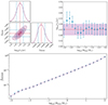 |
Fig. 2. These figure generalize the major results of the constraints on the fraction of MDMS, the core size of the Milky Way dark matter halo as well as the lens mass independence of the core size. Top left: corner plot of the two parameters fMDMS and core size rb with a lens mass of 10−2.2 M⊙. The solid red lines show the median value of the posterior distribution, and the dashed blue lines denote the 68% confidence interval. The yellow point shows the median value of the MCMC sampled posterior, and the different contours in the corner plot denote the different σ levels. Top right: core size as a function of the lens masses. The solid red line shows the median value from the left panel for rb, and the one σ range is plotted as the purple belt. The different core sizes sampled from different lens masses are shown as data points with error bars. The value remains almost unchanged within the one σ level. Bottom: fraction of MDMS fMDMS from the MCMC as function of the lens masses. The red points show the median, and the blue error bars show the one sigma range for each mass value. The solid purple line connects the median values. |
For a lens mass of about 10−3 M⊙, fMDMS surprisingly is about 10−3. This means that 109 M⊙ dark matter is in the form of MDMS at most, which is a much stronger constraint than was given by previous results (Niikura et al. 2019). The dependence of fMDMS on the lens mass arises from the cadence of the OGLE survey, which is in [0.1 days, 300 days]. As a result, when the lens mass is too high (> 1 M⊙) or too low (< 10−3 M⊙), the constraint on fMDMS approaches 1. The bottom panel of Fig. 2 clearly shows the dependence of fMDMS on the stellar lens mass, which is purely introduced by the OGLE survey cadence.
4. Discussion and summary
In the review of the density profile of dark matter halos by Paulo (Salucci 2019) concluded that the Milky Way dark matter halo has a core structure with a size between 1 and 100 kpc. Nesti & Salucci (2013) estimated the core size of Milky Way dark matter halo to be about 10 kpc using multiple dynamical data, such as the MW terminal velocities in the region inside the solar circle, the circular velocity as recently estimated from maser star-forming regions at intermediate radii, and the velocity dispersions of stellar halo tracers for the outermost Galactic region. The relation between our result and theirs is worth being probed if the smaller structure is an additional structure to the larger core.
Chan et al. (2015) generated a suite of simulations based on the same code of FIRE. They focused on the core size of galaxies with a wide range of stellar masses and feedbacks. Their results presented much larger core sizes than ours that ranged from 1.2 kpc to 2.0 kpc for the Milky Way dark matter halo. Our results show a much smaller core size that is caused by the baryonic feedback in the simulations.
This is a first attempt to constrain the core of the Milky Way dark matter halo using the OGLE microlensing sky map, and we realize the limitation of the OGLE data for our constraints. The OGLE survey targets the Milky Way bulge. Before we draw any solid conclusions about the implications for hydrosimulations and dark matter particle properties (as described in the next paragraph) based on the core size, we further explore other means to test our results. In another upcoming work, we select microlensing event candidates in the Milky Way halo using a technique called static microlensing (Guo et al. 2024; He et al., in prep.). We will further explore the core size based on these new data. In the future, powerful time-domain surveys such as the Legacy Survey of Space and Time (LSST) (Ivezić et al. 2019) and the Wide Field Survey Telescope (WFST) (Wang et al. 2023) will also provide valuable microlensing events in the Milky Way halo.
On the other hand, phenomenological models beyond the CDM provide another means to interpret the formation of the core structure. These means range from a solitonic core of ultralight dark matter (ULDM) (Kendall & Easther 2020) or fuzzy dark matter (FDM) (Burkert 2020) to self-interacting dark matter (SIDM) (Rocha et al. 2013) and weakly interacting massive particles (WIMP) (de Swart et al. 2017). However, the core size of the dark matter halo behaves differently in the stellar feedback scenario from one of these models, specifically, the SIDM model (Rocha et al. 2013). The hydro-simulation by Chan et al. (2015) shows the core size peaks around log10(M*/M⊙)∼10.0, while the SIDM illustrates a monotonic increase as a function of halo mass. In general, different models for dark matter particle might be tested by astrophysical observations, such as modulated Einstein rings from multiple-image systems of strong-lensing events (Amruth et al. 2023). We presented a novel method for probing the dark matter density profile with a microlensing sky map. This can be used to further constrain various mechanisms of core formation.
To summarize, we applied the OGLE microlensing sky map to obtain the tightest constraint on the core size of the Milky Way dark matter halo so far. The core size value is  and is independent of Mlens within a wide mass range. This result can potentially place stronger constraints on the cross section of SIDM particles and on the mass of ULDM/FDM. The core size can constrain the strength of the star formation process in the Milky Way. We acknowledge that we did not consider an off-center between the dark matter halo potential center and the Galactic center in our modeling. This can be another interesting issue to probe. We also note that the OGLE event-rate sky map we used is only located at the Galactic center, and more data beyond the Galactic center region will greatly improve the constraint based on our model.
In the future, when a wider survey range of microlensing event-rate maps (potentially Gaia archive data Gaia Collaboration 2021) or novel statistical measures of microlensing event-rate sky map are available, our method can be extended to a series of studies of the detailed structures of the Milky Way dark matter halo.
Acknowledgments
We are grateful to Shude Mao, Ruizhi Yang, Weicheng Zang, Elisa Ferreira, and Christopher J. Miller for valuable discussions. This work is supported in part byby NSFC (12192224, 12003029 11833005,92476203), National Key R&D Program of China (2021YFC2203100,2024YFC2207500), the Frontier Scientific Research Program of Deep Space Exploration Laboratory (No. 2022-QYKYJH-HXYF-012), by CAS young interdisciplinary innovation team (JCTD-2022-20), by 111 Project for “Observational and Theoretical Research on Dark Matter and Dark Energy” (B23042), by Fundamental Research Funds for Central Universities, by CSC Innovation Talent Funds, by USTC Fellowship for International Cooperation, by USTC Research Funds of the Double First-Class Initiative, by CAS project for young scientists in basic research (YSBR-006). Data availability. The code supporting this work is available from the corresponding authors upon reasonable request. The EMCEE package is available under MIT License in: https://emcee.readthedocs.io/en/stable/. The Ultranest package is available in https://johannesbuchner.github.io/UltraNest/. The microlensing modeling code is available in https://github.com/all2b9s/Static-microlensing. The OGLE catalogue is publicly available in: https://ogle.astrouw.edu.pl/.
References
- Amruth, A., Broadhurst, T., Lim, J., et al. 2023, Nat. Astron., 7, 736 [NASA ADS] [CrossRef] [Google Scholar]
- Bekki, K. 2009, MNRAS, 398, L36 [CrossRef] [Google Scholar]
- Birrer, S., Shajib, A. J., Galan, A., et al. 2020, A&A, 643, A165 [NASA ADS] [CrossRef] [EDP Sciences] [Google Scholar]
- Bozorgnia, N., & Bertone, G. 2017, Int. J. Mod. Phys. A, 32, 1730016 [NASA ADS] [CrossRef] [Google Scholar]
- Buchner, J. 2016, Stat. Comput., 26, 383 [Google Scholar]
- Buchner, J. 2019, PASP, 131, 108005 [Google Scholar]
- Buchner, J. 2021, J. Open Source Softw., 6, 3001 [CrossRef] [Google Scholar]
- Burkert, A. 1995, ApJ, 447, L25 [NASA ADS] [Google Scholar]
- Burkert, A. 2020, ApJ, 904, 161 [NASA ADS] [CrossRef] [Google Scholar]
- Calamida, A., Sahu, K. C., Casertano, S., et al. 2015, ApJ, 810, 8 [NASA ADS] [CrossRef] [Google Scholar]
- Carr, B., & Kühnel, F. 2020, Ann. Rev. Nucl. Part. Sci., 70, 355 [Google Scholar]
- Chan, T. K., Kereš, D., Oñorbe, J., et al. 2015, MNRAS, 454, 2981 [NASA ADS] [CrossRef] [Google Scholar]
- Croon, D., McKeen, D., & Raj, N. 2020, Phys. Rev. D, 101 [Google Scholar]
- de Blok, W. J. G. 2010, Adv. Astron., 2010, 789293 [CrossRef] [Google Scholar]
- de Swart, J. G., Bertone, G., & van Dongen, J. 2017, Nat. Astron., 1, 0059 [NASA ADS] [CrossRef] [Google Scholar]
- Del Popolo, A., & Le Delliou, M. 2022, ArXiv e-prints [arXiv:2209.14151] [Google Scholar]
- Delos, M. S., & Silk, J. 2023, MNRAS, 520, 4370 [NASA ADS] [CrossRef] [Google Scholar]
- Diemand, J., Kuhlen, M., Madau, P., et al. 2008, Nature, 454, 735 [NASA ADS] [CrossRef] [Google Scholar]
- Foreman-Mackey, D., Hogg, D. W., Lang, D., & Goodman, J. 2013, PASP, 125, 306 [Google Scholar]
- Gaia Collaboration (Brown, A. G. A., et al.) 2021, A&A, 649, A1 [NASA ADS] [CrossRef] [EDP Sciences] [Google Scholar]
- Gentile, G., Salucci, P., Klein, U., Vergani, D., & Kalberla, P. 2004, MNRAS, 351, 903 [Google Scholar]
- Guo, Q., Wei, L., Luo, W., et al. 2024, ArXiv e-prints [arXiv:2411.02161] [Google Scholar]
- Hikage, C., Oguri, M., Hamana, T., et al. 2019, PASJ, 71, 43 [Google Scholar]
- Ivezić, Ž., Kahn, S. M., Tyson, J. A., et al. 2019, ApJ, 873, 111 [Google Scholar]
- Jiang, F., Benson, A., Hopkins, P. F., et al. 2023, MNRAS, 521, 4630 [NASA ADS] [CrossRef] [Google Scholar]
- Karukes, E. V., & Salucci, P. 2017, MNRAS, 465, 4703 [Google Scholar]
- Kendall, E., & Easther, R. 2020, PASA, 37, e009 [NASA ADS] [CrossRef] [Google Scholar]
- Klypin, A., Zhao, H., & Somerville, R. S. 2002, ApJ, 573, 597 [Google Scholar]
- Kroupa, P. 2001, MNRAS, 322, 231 [NASA ADS] [CrossRef] [Google Scholar]
- Leauthaud, A., Saito, S., Hilbert, S., et al. 2017, MNRAS, 467, 3024 [Google Scholar]
- Mao, S., & Paczyński, B. 1996, ApJ, 473, 57 [NASA ADS] [CrossRef] [Google Scholar]
- Mao, Y.-Y., Strigari, L. E., Wechsler, R. H., Wu, H.-Y., & Hahn, O. 2013, ApJ, 764, 35 [NASA ADS] [CrossRef] [Google Scholar]
- Mróz, P., Udalski, A., Skowron, J., et al. 2017, Nature, 548, 183 [Google Scholar]
- Mróz, P., Udalski, A., Skowron, J., et al. 2019, ApJS, 244, 29 [Google Scholar]
- Mróz, P., Udalski, A., Szymański, M. K., et al. 2020, ApJ, 249, 16 [Google Scholar]
- Navarro, J. F., Frenk, C. S., & White, S. D. M. 1997, ApJ, 490, 493 [Google Scholar]
- Nesti, F., & Salucci, P. 2013, JCAP, 2013, 016 [Google Scholar]
- Niikura, H., Takada, M., Yokoyama, S., Sumi, T., & Masaki, S. 2019, Phys. Rev., D, 99 [Google Scholar]
- Novikov, I. D., Polnarev, A. G., Starobinskii, A. A., & Zeldovich, I. B. 1979, A&A, 80, 104 [NASA ADS] [Google Scholar]
- Planck Collaboration VI. 2020, A&A, 641, A6 [NASA ADS] [CrossRef] [EDP Sciences] [Google Scholar]
- Riess, A. G., Nugent, P., Filippenko, A. V., Kirshner, R. P., & Perlmutter, S. 1998, ApJ, 504, 935 [NASA ADS] [CrossRef] [Google Scholar]
- Rocha, M., Peter, A. H. G., Bullock, J. S., et al. 2013, MNRAS, 430, 81 [NASA ADS] [CrossRef] [Google Scholar]
- Salucci, P. 2019, A&ARv, 27, 2 [NASA ADS] [CrossRef] [Google Scholar]
- Salucci, P., & Burkert, A. 2000, ApJ, 537, L9 [NASA ADS] [CrossRef] [Google Scholar]
- Sasaki, M., Suyama, T., Tanaka, T., & Yokoyama, S. 2018, Class. Quant. Grav., 35, 063001 [NASA ADS] [CrossRef] [Google Scholar]
- Spergel, D. N., & Steinhardt, P. J. 2000, Phys. Rev. Lett., 84, 3760 [NASA ADS] [CrossRef] [Google Scholar]
- Verde, L., Treu, T., & Riess, A. G. 2019, Nat. Astron., 3, 891 [Google Scholar]
- Wang, J., Bose, S., Frenk, C. S., et al. 2020, Nature, 585, 39 [Google Scholar]
- Wang, T., Liu, G., Cai, Z., et al. 2023, Sci. China Phys. Mech. Astron., 66, 109512 [NASA ADS] [CrossRef] [Google Scholar]
- Wetzel, A., Hayward, C. C., Sanderson, R. E., et al. 2023, ApJ, 265, 44 [NASA ADS] [Google Scholar]
Appendix A: Model dependencies
In this supplementary material, we will discuss the model dependency of core size and fMDMS to show the robustness of our result.
A.1 Velocity distribution – In the main body of this paper, a Maxwell-Boltzmann distribution for MDMS is assumed. Still, as shown in cosmological simulations, there are other velocity distribution candidatesBozorgnia & Bertone (2017). So here we will discuss how different velocity distributions affect our results.
As shown in Mao et al, 1996Mao & Paczyński (1996), for lens with a given velocity |v|, the asymptotic behaviors of the event rate are given by:
 (A.1)
(A.1)
where the characteristic timescale is  . If we take the velocity distribution of the lens into account, we would need to integrate over |v|:
 (A.2)
(A.2)
As the velocity only takes value inside a limited interval due to f(v), the integrals hold asymptotically.
As we can see from Eq. A.2, for any given velocity distribution, it only results in an overall factor to the event rate for short-timescale and large-timescale events, which is independent of the angular position of the source. As the constraint of core size comes from the angular distribution of event rate, the velocity distribution will have no impact on the prediction of core size when the time scale of events is very short or very large. That is to say, the impact of velocity distribution on the prediction only comes from those events with tE ∼ tm.
To demonstrate the impact of the velocity distribution, here we use the model given in Mao et al. (2013) for the test:
 (A.3)
(A.3)
The result is shown in FIG. A.1. As we can see, even though the new model has a different mean velocity and velocity dispersion, the one-sigma range still overlaps with the previous one. This indicates the robustness of our result.
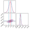 |
Fig. A.1. We use the velocity distribution given in Mao et al. (2013), with (v0/vesc, p)=(0.13, 0.78) and Mlens = 10−2.2 M⊙. Here the core size is |


A.2 Extended lens – For a point lens, the criterion for a micro-lensing event is:
 (A.4)
(A.4)
Here, Δsl is the distance between the lens and the projection of the source in the lens plane. RE is the Einstein radius.
When Δsl = RE, the total magnification μT = 1.34. If we keep this criterion, as shown in Croon et al, 2020Croon et al. (2020), the effect of an extended lens will result in an impact parameter u1.34 which serves as a modifying factor to RE. So, the micro-lensing event rate for extended will be:
 (A.5)
(A.5)
Here v′⊥ = (2u1.34REcosθ)/(tE).
To test the impact of the possible extended structure of MDMS, we take u1.34 = 0.4, 0.6, 0.8, 1, 1.2, 1.4, 1.6 (u1.34 is the case we showed in the main body of our paper) and rerun the whole analysis. The result is shown in FIG. A.2. For all the impact parameters we tested, the results are all within the one-sigma range of the point lens case(i.e. u1.34 = 1.0). This indicates that our result is still valid even when considering the extended structure of MDMS.
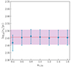 |
Fig. A.2. Here we have done tests with u1.34 = 0.4, 0.6, 0.8, 1, 1.2, 1.4, 1.6 and Mlens = 10−1.0 M⊙. As we can see, for different impact parameters, the results are still within the one sigma range of the fiducial value(i.e. u1.34 = 1.0.) |
A.3 Anisotropy of density profile – As discussed in Mróz et al. 2020 Mróz et al. (2020), the event rate observed in the northern hemisphere is lower than in the southern hemisphere. To examine the impact of this anisotropy, we consider the first-order perturbation of the density profile of MDMS:
 (A.6)
(A.6)
Here α is used to demonstrate the first-order anisotropy in the density profile
With this profile, we rerun the whole analyzing process with α as an additional parameter in the MCMC process. The result is shown in Fig. A.3. The result shows the density in the southern hemisphere is a little higher than the northern part (α = −0.008), which coincides with the OGLE observation. Also, the new core size, 240 pc, is still within the one-sigma range shown in the main body of our paper. So, to the first-order level, the core size we present here is not significantly affected by the anisotropy.
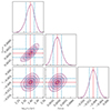 |
Fig. A.3. We use ρaniso defined in Eq. (A.6) to rerun the MCMC with α as an additional parameter. Here, Mlens = 10−2.2 M⊙. The core size is |


All Tables
Density profile and velocity profile for each type of lens, where α = dl/ds, κ = 5.625 × 10⁻³ km/s/pc, λ = 3.75 × 10⁻³ km/s/pc, δ = (8000 − x) pc, K0(x) is the modified Bessel function, and , s4 = R4 + (z/0.61)4, r2 = x2 + y2 + z2.
All Figures
|
Fig. 1. Sky maps in a Mollweide projection. Left panel: Microlensing event rate in an NFW density profile. Middle panel: Event rate for a core of 282 pc. Right panel: sky map of 5790 OGLE microlensing events. The difference between the graticules are 2 deg in longitude and 4.5 deg in latitude. As we are unable to reach all the detailed data of the microlensing events that were used to build the catalog, we cannot plot an event-rate sky map (see Fig. 24 of Mróz et al. 2020). |
| In the text | |
|
Fig. 2. These figure generalize the major results of the constraints on the fraction of MDMS, the core size of the Milky Way dark matter halo as well as the lens mass independence of the core size. Top left: corner plot of the two parameters fMDMS and core size rb with a lens mass of 10−2.2 M⊙. The solid red lines show the median value of the posterior distribution, and the dashed blue lines denote the 68% confidence interval. The yellow point shows the median value of the MCMC sampled posterior, and the different contours in the corner plot denote the different σ levels. Top right: core size as a function of the lens masses. The solid red line shows the median value from the left panel for rb, and the one σ range is plotted as the purple belt. The different core sizes sampled from different lens masses are shown as data points with error bars. The value remains almost unchanged within the one σ level. Bottom: fraction of MDMS fMDMS from the MCMC as function of the lens masses. The red points show the median, and the blue error bars show the one sigma range for each mass value. The solid purple line connects the median values. |
| In the text | |
|
Fig. A.1. We use the velocity distribution given in Mao et al. (2013), with (v0/vesc, p)=(0.13, 0.78) and Mlens = 10−2.2 M⊙. Here the core size is |
| In the text | |
|
Fig. A.2. Here we have done tests with u1.34 = 0.4, 0.6, 0.8, 1, 1.2, 1.4, 1.6 and Mlens = 10−1.0 M⊙. As we can see, for different impact parameters, the results are still within the one sigma range of the fiducial value(i.e. u1.34 = 1.0.) |
| In the text | |
|
Fig. A.3. We use ρaniso defined in Eq. (A.6) to rerun the MCMC with α as an additional parameter. Here, Mlens = 10−2.2 M⊙. The core size is |
| In the text | |
Current usage metrics show cumulative count of Article Views (full-text article views including HTML views, PDF and ePub downloads, according to the available data) and Abstracts Views on Vision4Press platform.
Data correspond to usage on the plateform after 2015. The current usage metrics is available 48-96 hours after online publication and is updated daily on week days.
Initial download of the metrics may take a while.