| Issue |
A&A
Volume 693, January 2025
|
|
|---|---|---|
| Article Number | A233 | |
| Number of page(s) | 17 | |
| Section | Astrophysical processes | |
| DOI | https://doi.org/10.1051/0004-6361/202452277 | |
| Published online | 21 January 2025 | |
Relativistic reconnection with effective resistivity
I. Dynamics and reconnection rate
1
Dipartimento di Fisica, Università di Torino, Via P. Giuria 1, I-10125 Torino, Italy
2
Université Paris-Saclay, Université Paris Cité, CEA, CNRS, AIM, F-91191 Gif-sur-Yvette, France
3
INFN – Sezione di Torino, Via P. Giuria 1, I-10125 Torino, Italy
4
Univ. Grenoble Alpes, CNRS, IPAG, 38000 Grenoble, France
5
Max-Planck Institute for Astronomy (MPIA), Königstuhl 17, 69117 Heidelberg, Germany
6
INFN, Sezione di Firenze, Via G. Sansone 1, I-50019 Sesto Fiorentino, (FI), Italy
7
Dipartimento di Fisica e Astronomia, Università di Firenze, Via G. Sansone 1, I-50019 Sesto Fiorentino, (FI), Italy
8
INAF, Osservatorio Astrofisico di Arcetri, Largo E. Fermi 5, I-50125 Firenze, Italy
9
INAF, Osservatorio Astrofisico di Torino, Strada Osservatorio 20, I-10025 Pino Torinese, (TO), Italy
⋆ Corresponding author; This email address is being protected from spambots. You need JavaScript enabled to view it.
Received:
17
September
2024
Accepted:
8
December
2024
Abstract
Context. Relativistic magnetic reconnection is one of the most fundamental mechanisms that is considered responsible for the acceleration of relativistic particles in astrophysical jets and magnetospheres of compact objects. Understanding the properties of the dissipation of magnetic fields and the formation of non-ideal electric fields is of paramount importance to quantify the efficiency of reconnection at energizing charged particles.
Aims. Recent results from particle-in-cell (PIC) simulations suggest that the fundamental properties of how magnetic fields dissipate in a current sheet might be captured by an “effective resistivity” formulation, which would locally enhance the amount of magnetic energy dissipated and favor the onset of fast reconnection. Our goal is to assess this ansatz quantitatively by comparing fluid models of magnetic reconnection with a non-constant magnetic diffusivity and fully kinetic models.
Methods. We performed 2D resistive relativistic magnetohydrodynamic (ResRMHD) simulations of magnetic reconnection combined to PIC simulations using the same initial conditions (i.e., a Harris current sheet). We explored the impact of crucial parameters such as the plasma magnetization, its mass density, the grid resolution, and the characteristic plasma skin depth.
Results. Our ResRMHD models with effective resistivity are able to quantitatively reproduce the dynamics of fully kinetic models of relativistic magnetic reconnection. In particular, they lead to reconnection rates consistent with PIC simulations, whereas for constant-resistivity fluid models, the reconnection dynamics is generally ten times slower. Even at modest resolutions, adopting an effective resistivity can qualitatively capture the properties of kinetic reconnection models and produce reconnection rates compatible with collisionless models (i.e., on the order of ∼10−1).
Key words: acceleration of particles / magnetic reconnection / magnetohydrodynamics (MHD) / plasmas / relativistic processes / methods: numerical
© The Authors 2025
 Open Access article, published by EDP Sciences, under the terms of the Creative Commons Attribution License (https://creativecommons.org/licenses/by/4.0), which permits unrestricted use, distribution, and reproduction in any medium, provided the original work is properly cited.
This article is published in open access under the Subscribe to Open model. This email address is being protected from spambots. You need JavaScript enabled to view it. to support open access publication.
1. Introduction
Relativistic magnetic reconnection is one of the main physical processes invoked to explain the high-energy emission produced by strongly magnetized astrophysical plasmas. Its core mechanism consists of the rearrangement of magnetic field lines, which rapidly transfers the magnetic energy stored in the plasma into heat, high-speed flows, and accelerated particles. This process is believed to power a large number of highly energetic peculiar transients, such as flares from black hole magnetospheres (Nathanail et al. 2022; Ripperda et al. 2022), pulsar magnetospheres (Lyubarskii 1996; Uzdensky & Spitkovsky 2014) and pulsar wind nebulae (Cerutti et al. 2012a; Olmi et al. 2016), fast radio bursts Mahlmann et al. (2022), Most & Philippov (2023), gamma-ray bursts Zhang & Yan (2011), McKinney & Uzdensky (2012), and flares from blazar jets (Giannios 2013; Petropoulou et al. 2016).
Particle in cell (PIC) numerical simulations are an essential numerical tool to model the fundamental physics behind the reconnection of current sheets in astrophysical plasmas (Zenitani & Hoshino 2001; Cerutti et al. 2012b; Sironi & Spitkovsky 2014). Their ability to capture the collisionless nature of astrophysical plasmas makes it possible to quantitatively model the dissipation of magnetic fields and the consequent acceleration of relativistic particles from first principles. However, their high computational cost poses a serious challenge when working to address the large separation between typical length scales of the plasma (e.g., particles gyroradius, plasma skin depth) and the size of the astrophysical systems where reconnection takes place. On the other hand, resistive relativistic magnetohydrodynamics (ResRMHD; see, e.g., Komissarov 2007; Palenzuela et al. 2009) offers a powerful framework to study the impact of magnetic dissipation on the large-scale dynamics of accretion flows around compact objects (Qian et al. 2017; Ripperda et al. 2019a; Vos et al. 2024) and the launch of relativistic polar outflows (Mattia et al. 2023, 2024). By introducing an explicit physical magnetic diffusivity, such simulations can quantitatively address the formation of current sheets and the departure from an ideal relativistic magnetohydrodynamic (RMHD) regime (Del Zanna et al. 2016), while also decoupling the dissipation properties from the specific numerical implementation of the code adopted. Nonetheless, such resistivity is only a proxy for the actual magnetic dissipation occurring in the plasma, as its value is typically assumed to be constant across the domain and is significantly limited by the numerical diffusion imposed by the grid discretization. Moreover, reconnection rates produced by fluid models are generally one order of magnitude lower than those obtained with fully kinetic models (Sironi & Spitkovsky 2014), suggesting a fundamental shortcoming in the ability of ResRMHD simulations to capture the properties of collisionless reconnection.
One possible way to improve the description of magnetic dissipation in the ResRMHD framework is to introduce an “anomalous resistivity” in specific regions close to the current sheet, where the dissipation is significantly enhanced Watanabe & Yokoyama (2006), Zanotti & Dumbser (2011). Such an approach can significantly increase the rate at which magnetic field lines are reconnected, but it requires one to select a priori a fraction of the numerical domain where dissipation needs to be amplified. Some works have instead adopted the more practical strategy to increase resistivity in regions with high values of current density Zenitani et al. (2010), Ripperda et al. (2019b), which is more flexible and can deal with non-trivial configurations of the current sheet. This prescription can lead to faster reconnection as well, but the amplitude of the “effective” resistivity was still set by an arbitrary constant that was not constrained by a specific physical model of collisionless reconnection. Selvi et al. (2023) provided the first physically motivated model for effective resistivity informed by first-principles PIC simulations of 2D Harris sheets that is consistent with a classical collisionless inertial resistivity associated with a finite permanence of charged particles within the reconnecting region (Speiser 1970). By measuring the dominant component of the electric field within the reconnecting layer in the comoving frame and comparing it to the local current density, they constructed a closed form for an effective resistivity, ηeff, that depends on the particles’ mean velocity and density.
The present study is aimed at testing, for the first time, the prescription proposed by Selvi et al. (2023) by using 2D ResRMHD models of magnetic reconnection. We reformulated the expression for the effective resistivity in terms of fluid quantities available in MHD models and measured its effects on the dynamics of a standard 2D Harris current sheet, quantifying the impact of the different quantities that set its magnitude. By performing a set of PIC simulations sharing the same initial conditions as the fluid models, we quantified the accuracy of the effective resistivity prescription to capture the non-collisional properties of magnetic dissipation, obtaining a very good agreement between the two numerical frameworks.
Our study takes the following structure. In Sect. 2, we introduce the numerical methods we adopted and the derivation of the closed form of ηeff we use in the rest of the paper. In Sect. 3, we present a detailed analysis of the reconnection dynamics introduced by the effective resistivity and the comparison with the constant resistivity and kinetic cases. In Sect. 4, we quantify the impact of numerical dissipation (through a convergence study) and physical parameters (e.g., magnetization, density, and plasma skin depth) in combination with PIC models. Finally, we share our conclusions in Sect. 5 and present numerical benchmarks validating our resistivity implementation in Appendix A. We leave the analysis of the particle acceleration process and the impact of effective resistivity on their spectral distribution to an upcoming follow-up study. We use CGS Gaussian units throughout the paper.
2. Numerical methods
2.1. Resistive RMHD models
Our ResRMHD simulations were performed using the PLUTO code Mignone et al. (2007). We solved a set of conservation laws that take the form:
 (1)
(1)
with the vectors of conservative variables U and fluxes F given by
 (2)
(2)
Here, D = Γρ is the mass density of the plasma,  is the total momentum density, ℰ = ρc2hΓ2 − p + uem is the total energy density,
  is the total stress tensor, B is the magnetic field, E is the electric field (all measured in the laboratory frame), and εijk is the 3D Levi-Civita symbol. In the previous expressions we introduced the Lorentz factor, Γ, the electromagnetic energy density,
  , the total pressure, ptot = p + uem, and the specific enthalpy, h, along with the so-called “primitive” variables, namely: the rest mass density, ρ, the fluid spatial velocity, v, or the related spatial part of the four-velocity, u = Γv (then
  ), and the thermal pressure, p.
The source term vector in Eq. (1) is instead given by
 (3)
(3)
where the current density, J, is expressed in terms of primitive variables and the electromagnetic field using the relativistic Ohm’s law for a resistive plasma (Komissarov 2007):
![Mathematical equation: $$ \begin{aligned} \boldsymbol{J} = \rho _e\boldsymbol{v} + \frac{1}{\eta } \Gamma \left[\boldsymbol{E} + \frac{1}{c}\boldsymbol{v}\times \boldsymbol{B} -\frac{1}{c^2}(\boldsymbol{E}\cdot \boldsymbol{v})\boldsymbol{v}\right], \end{aligned} $$](/articles/aa/full_html/2025/01/aa52277-24/aa52277-24-eq8.gif) (4)
(4)
where ρe is the electric charge density and η is the electric resistivity, taken here as the inverse of the fluid conductivity.
A well-known property of the evolution equation for the electric field, as first pointed out by Komissarov (2007), is that it can be potentially stiff for low values of the magnetic resistivity, since parts of its source term (i.e., those inversely proportional to η) change over characteristic timescales that may end up being much shorter than the rest of the contributions (Palenzuela et al. 2009; Bucciantini & Del Zanna 2013; Del Zanna & Bucciantini 2018). To ensure numerical stability to the time integration of Eq. (2), we used the IMEX-SSP3(3,3,2) scheme (Pareschi & Russo 2005), following a similar procedure to the one presented in Mignone et al. (2019) and Tomei et al. (2020).
The evolutionary laws described in Eqs. (1), (2), and (3) need to be coupled to the solenoidal constraint for the magnetic field and the conservation of electric charge, namely:
 (5)
(5)
 (6)
(6)
While we enforced the diverge-free condition by using staggered magnetic field components via the Constrained Transport (CT) method (Londrillo & del Zanna 2004), we used the latter equation to compute the electric charge without enforcing the electric field divergence (Bucciantini & Del Zanna 2013). All our models were performed using also WENOZ (Castro et al. 2011) reconstruction and the MHLLC Riemann solver (Mignone et al. 2019).
2.1.1. Effective resistivity model
In this subsection, we describe our implementation in the PLUTO code of the effective resistivity model proposed by Selvi et al. (2023), which pertains exclusively to a pair plasma without guide field. Using 2D fully kinetic relativistic PIC models of reconnecting Harris sheets, Selvi et al. (2023) measured the resistive component of the electric field produced within the current sheet and compared it to the general expression for the relativistic Ohm law Hesse & Zenitani (2007). In their model, the sheet is aligned with the x-axis, the y direction is transverse to it, and the z-axis is a symmetry axis perpendicular to the plane containing the initial magnetic field (i.e., no guide field is included). They identified the effective resistivity parameter as the ratio between the out-of-plane components of the comoving electric field and the current density and then estimated the dominant terms contributing to the electric field in the co-moving frame of the fluid (which is expected to vanish only in the limit of a perfectly conducting plasma), obtaining:
 (7)
(7)
where m is the mass of the electron, nt is the plasma number density, e is the electron charge, uαz is the z-component of the four-velocity of the species α (in our case, either an electron or a positron), vαz is the z-component of its three-velocity, and ⟨⟩ represents an average over the particle distribution. It should be noted that Eq. (7) is not covariant and its validity is limited (a priori) to the fluid comoving frame (given the expression of the Ohm law used by Selvi et al. 2023). While a covariant formulation would be much preferable, in the absence of fast bulk motions (as is the case here) there should not be any strong deviations in the effective resistivity. To express the effective resistivity exclusively in terms of fluid quantities that are available in an RMHD simulation, we can first approximate the ratio ⟨uαz⟩/⟨vαz⟩ with the electron Lorentz factor, Γe, and introduce the fluid rest-mass density, ρ = mnt, as well as the y-component of the fluid velocity vy ≈ ⟨vαy⟩, using charge neutrality and symmetry reasons. If we go on to express Γe in terms of the current density (i.e., ρe⟨vei⟩/m ≃ ji) we can use the fact that for a 2D current sheet with no guide field, the only non-vanishing component of the current density is the out-of-plane one. We thus obtain
 (8)
(8)
This relation corresponds to a form of the effective resistivity for a fluid code proposed in an earlier version of Selvi et al. (2023) and can be rewritten as
 (9)
(9)
where we define the quantities E0 = (mc/e)∂yvy and J0 = ρec/m. By substituting jz = ez/ηeff and solving for ηeff, we can finally obtain
 (10)
(10)
where
![Mathematical equation: $$ \begin{aligned} \boldsymbol{e} = \Gamma \left[\boldsymbol{E} + \frac{1}{c}\boldsymbol{v} \times \boldsymbol{B}\right] \end{aligned} $$](/articles/aa/full_html/2025/01/aa52277-24/aa52277-24-eq17.gif) (11)
(11)
is the electric field in the fluid frame (e.g., Mignone et al. 2019).
Compared to Eq. (8), this expression for the effective resistivity has no singularities and is completely determined by fluid quantities readily available at each time step (whereas the current density would, in principle, require us to know the instantaneous value of the displacement current). More importantly, Eq. (10) has the benefit of producing a profile of resistivity that systematically peaks within the current sheet and tends to smoothly decrease once dissipation flattens the magnetic field profile (see Appendix A.2 for a 1D numerical test), thus leading to physically motivated dynamics, despite the strong approximations used in its derivation.
2.1.2. Numerical implementation
Equation (10) needs to be properly expressed in a dimensionless form, if we want to employ it within a resistive RMHD code. This is due to the fact that the fluid equations are scale-free in the limit of a constant scalar resistivity that does not depend on fundamental physical constants. We use Lu and ρu to indicate, respectively, the unit length and mass density that we adopted to rescale the variables appearing in Eq. (10) in terms of corresponding dimensionless quantities (indicated in the following with a bar notation), thus obtaining:
 (12)
(12)
In the previous expression, we rescale the electric (and magnetic) field according to  and we introduce the dimensionless plasma skin-depth,
  , with
  being the plasma frequency associated with the chosen unit of mass density. We can then obtain an expression for the dimensionless resistivity
  by factoring out the physical units in Ampère-Maxwell’s law as
![Mathematical equation: $$ \begin{aligned} \frac{\partial \bar{\boldsymbol{E}}}{\partial \bar{t}} - \bar{\boldsymbol{\nabla }} \times \bar{\boldsymbol{B}} = - \bar{\boldsymbol{J}} \equiv - \bar{\rho }_e \bar{\boldsymbol{v}} - \frac{1}{\bar{\eta }_{\rm eff}} \Gamma \left[\bar{\boldsymbol{E}} + \bar{\boldsymbol{v}} \times \bar{\boldsymbol{B}} - (\bar{\boldsymbol{E}} \cdot \bar{\boldsymbol{v}}) \bar{\boldsymbol{v}}\right], \end{aligned} $$](/articles/aa/full_html/2025/01/aa52277-24/aa52277-24-eq23.gif) (13)
(13)
which leads to this final form for the effective resistivity employed in the PLUTO code
 (14)
(14)
From Eq. (14), we can see how adopting the effective resistivity prescription introduces a characteristic scale to the problem,  , which is set by the specific choice of physical units for lengths and mass densities adopted by the code. This length scale represents a crucial parameter that determines the magnitude of the effective resistivity and it has a clearly defined physical meaning. For this reason, when we use Eq. (14), we set the amount of magnetic dissipation not by arbitrarily choosing a constant resistivity, η0; rather, we properly set an equivalent plasma skin-depth length scale and a density profile for the current sheet. Since the value of
  is a direct consequence of the physical units adopted by the code and the initial scale of the problem, we treat it as a fixed parameter that does not dynamically change with the local plasma skin depth (the dependence of ηeff on ρ already captures this effect). We compute the spatial derivative of the velocity component transverse to the current sheet via central differences and applying a minmod limiter to avoid spurious oscillations that would otherwise affect the resistivity profile. We also set a floor value of ηfloor = 10−6 in order to avoid excessively small values of resistivity that would simply hinder the stability of the code without significantly affecting the simulation’s dynamics (Ripperda et al. 2019a).
2.2. PIC models
Our simulations of collisionless magnetic reconnection are produced with the 2D version of the relativistic electromagnetic PIC code Zeltron (Cerutti et al. 2013; Cerutti & Werner 2019), which solves the time-dependent Maxwell equations
 (15)
(15)
 (16)
(16)
using a second-order finite-difference time-domain method (Yee 1966). While the divergence-free condition for the magnetic field is ensured to machine precision at any given time, the Gauss equation ∇ ⋅ E = 4πρe is enforced by applying at each time step a correction δE to the electric field obtained by solving Poisson’s equation:
 (17)
(17)
where ρe is the electric charge density and δE = −(∇δϕ). The electromagnetic field is coupled to the dynamics of the charged particles through their equation of motion
 (18)
(18)
where m is the particle’s mass, up = Γpvp is its 4-velocity, vp is its spatial velocity, q is its electric charge,  is its Lorentz factor, and {Ep, Bp} are the electric and magnetic fields at the particle’s location. The equation of motion is integrated using the classic Boris pusher (Birdsall & Langdon 1991). Charges and currents generated by each particle are then deposited on the nodes of the grid via linear interpolation, where they are used to compute the charge and current densities for Maxwell’s equations. In this work, we assume a pure electron-positron pair plasma, as in Selvi et al. (2023).
2.3. Initial conditions
We initialized our domain with a standard Harris current sheet of width a. In the following, quantities with subscript “0” refer to the upstream region of the domain (i.e., far from the current sheet). The magnetic field has non-vanishing component only along the x-axis, which is defined as
 (19)
(19)
where B0 is set by the plasma “cold” magnetization to σ0 = B02/ρ0 and the plasma density, ρ0 (here  for convenience). Once we have chosen the ratio of thermal to magnetic pressure β0 = 2p0/B02 (where p0 is the upstream plasma thermal pressure), we can compute the Alfvén speed as in Del Zanna et al. (2016)
 (20)
(20)
where we assume an ideal equation of state for a relativistic plasma with adiabatic index of 4/3. The thermal pressure, p, is then computed by requiring a constant total pressure of ptot = p + Bx2/2 in all the domain. This gives
 (21)
(21)
which we then use to compute the density across the domain by assuming an initial constant temperature, Θ = p/ρ = 1. This choice leads the upstream plasma density ρ0 to increase by a factor of p(0)/p0 = (β + 1)/β ≃ β−1 = 100 within the current sheet.
The magnetic field is expressed in terms of a vector potential along the z direction
 (22)
(22)
where the second term of the z-component introduces a sinusoidal perturbation with wavelength, L0, and amplitude, ϵ = 0.05, that is localized in proximity of the current sheet to seed the tearing instability in the ResRMHD models and predefine the location of the main X and O points along the sheet.
Our numerical domain consists of a Cartesian box with a uniform grid spacing equal to Δx ≃ δ0/20 (unless otherwise stated), where δ0 = c/ω0 is the upstream plasma skin-depth and ω0 is the corresponding plasma frequency. Our box covers the range of [0, 4L0] in the x-direction, where L0 = 1 is the characteristic length of the current sheet, while we set the current sheet width a = 0.01L0 = δ0/2. This length is 500 times the current sheet skin-depth δp, since ωp ≃ 10ω0. Throughout this work we consider values for the dimensionless skin-depth parameter  in Eq. (14) corresponding to either the upstream or the current sheet plasma skin-depth; namely,
  . Imposing a specific value to
  and assuming L0 = Lu is equivalent to setting the unit of mass density to
  , with re being the classical electron radius. Since the rest of the MHD equations remain scale-free, this adjustment does not affect the dynamics of the system any further. The size of our numerical box in the direction transverse to the current sheet needs to be sufficiently large so as to avoid artificial high-energy cutoffs in the spectra of particles accelerated by the reconnection electric field. Werner et al. (2016) showed that when the size of the domain in the direction transverse to the current sheet is not sufficiently large, namely, when
 (23)
(23)
the spectra of particles with mean Larmor radius, rL, that are accelerated by the reconnection electric field exhibit an artificial high-energy cutoff. We conservatively doubled the constraint from Eq. (23) and set ![Mathematical equation: $ y\in[-80\sqrt{\sigma_0}a,80\sqrt{\sigma_0}a] $](/articles/aa/full_html/2025/01/aa52277-24/aa52277-24-eq43.gif) , where we applied
, where we applied  . We imposed in the x- and y-direction periodic and reflective boundary conditions, respectively.
In the PIC simulations, the plasma is generated with 32 particles per cell everywhere in the domain. The initial density gradient in the layer is achieved thanks to variable particle weights. The initial particle energy distribution follows a relativistic Maxwellian at rest in the upstream medium, while the plasma in the layer is generated according to two counter-streaming relativistic drifting Maxwellian carrying the current (one beam for each species drifting at vdrift = ±0.6c along the z-direction). All kinetic models start with the same initial plasma skin depth as the ResRMHD case (i.e., 0.02L0 upstream, 0.002L0 at the center of the current sheet), the same numerical box, and a uniform grid spacing of Δx = δ0/10.
3. Effective resistivity models
3.1. Current sheet dynamics
We start with a brief description of the main properties of kinetic model s10pic, which represents a realization from first principles of the reconnection of the current sheet considered in this study. In the following, we measure space and time in units of L0 and L0/c, respectively. The initial equilibrium is promptly destroyed by a violent fragmentation of the current sheet in multiple magnetic islands that start merging and producing ever larger plasmoids, with a single large magnetic island remaining once saturation is reached. Figure 1 shows a snapshot taken at t ≃ 2.4 to showcase this well-known dynamics. A chain of four large high-density magnetic islands is interrupted by a series of small plasmoids that are about to merge with the larger O-points (top panel). Regions of intense resistive electric field develop in between plasmoids and at the interface of merging magnetic islands (bottom panel). The ratio between this electric field component and the current density (middle panel) represents the quantity that we refer to as the effective resistivity of the system. To avoid spurious high values in the upstream regions due to exceedingly low current densities, we do not render this ratio wherever the current density’s magnitude drops below a factor 10−2 with respect to its maximum at the beginning of the simulation. We can see a clear anti-correlation with mass density in the low resistivity regions at the core of each plasmoid, while high values of ez/jz are reached in correspondence to high values of the resistive electric field. This relations are both in agreement with the dependencies included in Eq. (14) that we previously introduced.
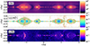 |
Fig. 1. Spatial profiles of (from top to bottom) mass density, ratio of comoving electric field over current density ez/jz, and ez for the kinetic model s10pic at t ≃ 2.4. The density is normalized by the upstream value, ρ0, the electric field by the upstream magnetic field, B0, and the current density by |

We go on to analyze models s10eEr1 and s10eEd0r1 to provide a reference for the reconnection dynamics produced by the effective resistivity prescription (a complete list of the simulations included in this work is presented in Table 1). Here, we consider a simulation with Nx = 4096 points along the x-axis (which corresponds to Δx = δ0/20, namely, twice the resolution used in the corresponding PIC simulation). A deeper analysis of the impact of numerical dissipation is undertaken in Sect. 4.1. As a reference, for a given resolution the PIC models require about twice as much computational resources with respect to the ResRMHD models. The employment of AMR in the grid structure would have further reduced the computational cost of the fluid models (especially in the upstream region, where it is enough to use a coarser resolution), but we opted for a uniform grid in order to more closely match the one used by PIC simulations.
ResRMHD and PIC models and their parameters: upstream “cold” magnetization, Alfvèn speed, resistivity, effective plasma skin depth, upstream density, and magnetic field.
In Fig. 2, we show a space-time diagrams of several quantities at the center of the reconnecting layer (similarly to Fig. 2 of Nalewajko et al. 2015, although for ResRMHD simulations rather than PIC). At the beginning of the simulation the current sheet becomes thinner by ≃20% due to the onset of the tearing instability, with the initial perturbation inducing the formation of a small magnetic island at x = 1 around t ≃ 1.7 (top-left panel of Fig. 2). During this phase, the resistivity remains relatively low (∼10−5) close to the two large X and O points forming in x = ±1 (top right panel). After this phase, the tearing instability enters its non-linear stage, with the current sheet beginning to also fragment into smaller plasmoids. The resistivity increases by more than an order of magnitude in between the smaller magnetic islands (where density decreases), as does the electric field in the plasma comoving frame. At t ≃ 2.5, the initial chain of small plasmoids starts to merge towards x = ±1, and by t ≃ 4 two large magnetic islands are left. Then, newly formed plasmoids continue to quickly merge toward them throughout the simulation. Both the resistivity and the non-ideal electric field spike in the low-density regions of the current sheet’s center at the sides of the plasmoids, with a clear correlation between them (top-right and bottom-left panels of Fig. 2). These regions, which are sparsly distributed, also produce favorable conditions for the acceleration of particles, as indicated by the negative values assumed by the Lorentz invariant B2 − E2 (Sironi 2022). The O-point formed in x = −1 around t ≃ 4 instead slowly approaches the lower periodic boundary of the x axis and merges across it with the original island around t ≃ 18. This halts the further reconnection of magnetic field lines, which leads to a drop of the non-ideal electric field on the sides of the last plasmoid and the relaxation towards a global saturated state with a single large plasmoid.
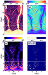 |
Fig. 2. Space-time diagrams of different quantities at the center of the current sheet (y = 0) over time for the ResRMHD model s10eEr1. From top left to bottom right: Rest-mass density ρ, effective resistivity ηeff, z-component of the electric field in the fluid frame ez, and Lorentz invariant B2 − E2. The white dotted lines indicate the instant where the profiles in Fig. 3 are shown. |
Figure 3 shows the profiles of a series of quantities at t = 6.3 for model s10eEr1, when the two largest plasmoids are steadily merging with smaller ones. The morphology of the reconnecting layer is consistent with the standard scenario produced by both kinetic and fluid models: the fragmentation of the current sheet produces a continuous coalescence of newly formed small structures into larger magnetic islands, with thin current filaments connecting them. The effective resistivity is larger around and in between the plasmoids, with strong peaks emerging at the interface of merging islands and in agreement with the results obtained by model s10pic. The non-ideal electric field also reaches its maximum value in these regions, but it is otherwise stronger within the magnetic islands, rather than at the edges. These regions also host the most promising sites for the initial phases of particle acceleration, with negative values of B2 − E2 reached in small patches in the middle of highly resistive parts of the current sheet. The last panel of Fig. 3 shows how the highest temperatures are reached not only around the dense core of the two largest plasmoids, but also in the rarefied regions of strong magnetic dissipation and non-ideal electric field, followed by the regions between magnetic islands where the electric field and the resistivity both peak.
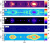 |
Fig. 3. Spatial profiles of (from top to bottom) the rest-mass density, ρ, the effective resistivity, ηeff, the z-component of the electric field in the fluid frame, ez, the Lorentz invariant, B2 − E2, with the contours of the vector potential, Az, and the temperature for the ResRMHD model s10eEr1 at t = 6.3. |
Model s10eEd0r1, for which the value of  is ten times greater, shows a similar initial transient in terms of current sheet thinning and fragmentation. However, both resistivity and electric field are initially weaker than the previous case (top right and bottom left panels of Fig. 4). In the non-linear stage of the simulation, we still have two large plasmoids forming at x = ±1 and merging together on the right side of the numerical box, but the process is faster and leads (by t ≃ 12L0/c) to a saturated state. Both resistivity and electric field still exhibit a very good correlation, but they are now much stronger and cover larger fractions of the current sheet’s length. This is accompanied by a clear lack of production of short-lived small plasmoids between the two main magnetic islands, where the density generally drops by more than an order of magnitude. The regions with favorable conditions for particle acceleration (bottom right panel) are now much larger and last longer in time, consistently with the aforementioned dissipation dynamics.
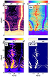 |
Fig. 4. Same as Fig. 2, but for the ResRMHD model s10eEd0r1. The white dotted lines indicate the instant at which the profiles in Fig. 5 are shown. |
The spatial profiles of such quantities at t = 4.5 (when the activity within the current sheet is most intense) are also qualitatively different than the case using  (Fig. 5). Both resistivity and non-ideal electric field reach their maximum values in the regions of low density (i.e., between the high-density merging plasmoids), which is consistent with the effective resistivity being inversely proportional to ρ. However, rather than having thin patches in between merging magnetic islands, we now have large, rarefied cavities with turbulent edges, which disrupt the current sheet and prevent the formation of chains of small-scale plasmoids. These regions also host the most promising sites for particle acceleration, with negative values of B2 − E2 reached in patches that are considerably larger than those produced in model s10eEr1. The high temperatures reached between plasmoids (last panel) confirm that such bubbles are produced by an excess of magnetic dissipation due to the much larger resistivity that comes with a larger value of
  . Such an evolutionary scenario deviates significantly from the reconnection dynamics produced by the self-consistent PIC model, thereby representing a limiting case for the effective resistivity formulation. This effect suggests that the layer thickness is set by the plasma skin depth scale in the sheet rather than in the upstream medium, which makes more sense physically. Model s10eEr1 will therefore serve as our reference run for the rest of the paper.
3.2. Global evolution of the magnetic field
The onset of the tearing instability triggered by the magnetic seed perturbation leads to an initial fast growth of the RMS y-component of the magnetic field (top panel of Fig. 6). The initial transient corresponding to the linear phase of the instability lasts roughly until t ≃ 2.5, at which point the fragmentation of the current sheet into smaller plasmoids induces an even faster increase of the reconnected magnetic field. The growth rate in this stage is roughly the inverse of the ideal time scale τA = L0/cA, which is even faster than the value predicted by the “ideal tearing” regime (Pucci & Velli 2014; Landi et al. 2015), namely, ≃0.6τA−1. Such a value corresponds, in principle, to a specific choice of aspect ratio for the current sheet (i.e., L/a = S1/3) and becomes smaller for thicker current sheets according to (Del Zanna et al. 2016; Komissarov & Phillips 2024):

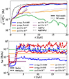 |
Fig. 6. RMS value of the transverse component of the magnetic field (top) and values of the resistivity (bottom) over time for ResRMHD models s10eEr1 (blue curve), s10eEd0r1 (red), models with constant resistivity (green, yellow, light purple, and purple), and model s10pic (dotted). The maximum and average values of the resistivity are calculated over a rectangular box of sizes Lx × 2a centered on y = 0. |
However, since the system is unstable on dynamical time scales when the current sheet reaches this thickness, obtaining a smaller value of a/L (hence faster reconnection) is hindered by the fragmentation of the current sheet itself. The growth rate γmax = 0.6τA−1 can therefore be considered an upper limit to what can be produced by a reconnection event in the ResRMHD regime with constant resistivity. After t ≃ 7.5, there is no significant growth of this quantity for model s10eEd0r1 as the system has reached a fully saturated state. The model with a lower value for  produces almost the same evolution for ⟨By2⟩, with only marginally slower growth after t ≃ 4. Overall, the corresponding PIC simulation (black dotted line) produces a very similar evolution as well. The growth of ⟨By2⟩ in the kinetic model is fast and steady, with a rate of increase that is close to the one experienced by the ResRMHD simulations after t ≃ 2.5; namely, this is the moment when their current sheet starts fragmenting. When the RMS field reaches the value ∼0.1B0, the field in the PIC simulation quickly saturates to the same intensity as for the fluid models (≃0.3B0). The difference between the initial transients occurring in the fluid and kinetic models stems from the fact that the former needs to go through a thinning of the current via the tearing instability, before reaching the point where the first plasmoids can form. On the other hand, the current sheet in model s10pic fragments immediately, therefore producing without delays a powerful reconnection event.
As previously seen, the effective resistivity assumes a wide range of values during the simulation. In the bottom panel of Fig. 6, we show the evolution over time of the average resistivity in the current sheet (specifically, within a distance a from the center) and the maximum value it assumes within the same region for models s10eEr1 and s10eEd0r1. We report it in units of B0/ρ0, since it is a quantity appearing from Eq. (14) that provides a natural scaling unit. During the linear phase of the tearing instability the average resistivity increases immediately from the initial floor value of ≃3 × 10⁻⁷B0/ρ0, due to the local resistive electric field building up (bottom left panels of Figs. 2 and 4). The increase ranges from a few (model s10eEr1) up to ten times (model s10eEd0r1), depending on the value of  . Around t ≃ 2.5, the resistivity then grows by up to three orders of magnitude due to the current sheet beginning to fragment, with a steady mean value at the center of the current sheet of roughly either 3 × 10⁻⁵B0/ρ0 (s10eEr1) or 2 × 10⁻³B0/ρ0 (s10eEd0r1). There is also a difference between the two models that is greater than the ratio between the two plasma skin-depths used by these models. This is due to the fact that the non-ideal electric field in model s10eEd0r1 is stronger than the one produced with a smaller value of
  , hence, the local dissipation rate is increased even more. After this fast increase in resistivity, both the average and maximum values do not vary much over time, with a ratio between the two rising up to ∼500. However, in model s10eEr1, the maximum value of ηeff right after the formation of the first plasmoid chains (t ≃ 2.5) decreases steadily by a an order of magnitude over the period required by the reconnected magnetic field to saturate, whereas such a decrease does not occur in the case of larger
  .
.
To quantify the efficiency of reconnection in our models, we first computed (for both the ResRMHD and PIC simulations) the reconnected magnetic flux Φrec along the current sheet (y = 0) as
 (24)
(24)
where we identify the position of the X (O) point by the maximum (minimum) value of Az. For both models with effective resistivity, the reconnected magnetic flux starts increasing significantly from t ≃ 2.5 (i.e., when the current sheets start fragmenting). Model s10eEr1 produces a rather steady growth of the magnetic flux, slowly saturating towards Φrec ≃ 0.5Φ0 by t ≃ 40, where Φ0 = B0Ly/2 is a measure of the magnetic flux available for reconnection at the beginning of the simulation. The flux from model s10eEd0r1 increases instead at a faster pace, it slows down after t ≃ 8.5 (due to the merger between the two last plasmoids being slower at the beginning) and then saturates at a similar value. Such deviation from the model with lower  reflects the faster and more violent reconnection dynamics produced by this model. Similarly to the evolution of By, the PIC simulation shows an immediate growth of the reconnected flux shortly after the beginning of the simulation, since the current sheet does not undergo a preliminary linear stage of the tearing instability. Besides this small offset, however, the evolution of the reconnected flux of the PIC model is very similar to that of the ResRMHD ones. The initial growth of Φrec falls roughly in between the two fluid models, halting briefly before the merger of the two last large magnetic islands and then saturating close to 0.5Φ0 as well.
We also computed the corresponding reconnection rates, βrec, as
 (25)
(25)
where we identify the inflow velocity of the magnetic field lines into the X-point with vrec = B0−1dΦrec/dt. Besides the delay between PIC and ResRMHD models, the reconnection rates obtained with the effective resistivity formulation are remarkably similar to the kinetic result. In the s10eEd0r1 simulation, we see that βrec spikes to a maximum value of ≃0.2 at the start of the current sheet fragmentation, which lasts until t ≃ 6. Model s10eEr1 produces a qualitatively comparable scenario, with a peak around ≃0.1 and a steadier mean value over time, which is consistent with the less dramatic increase in resistivity with respect to the case having  . Finally, PIC and ResRMHD models exhibit a very similar time variability, on both shorter and longer timescales.
3.3. Comparison with the uniform resistivity case
Our four models with constant and uniform resistivity profiles (s10eC2r1 to s10eC5r1) show the profound impact that the adoption of effective resistivity has on the reconnection dynamics. The magnetic dissipation η0 ranges from 2.5 × 10⁻² to 2.5 × 10⁻⁵, with the corresponding macroscopic Lundquist number, S = LcA/η going from ≃37.8 to ≃3.78 × 10⁴. All models were produced with the same resolution as the previous ones, namely, Nx = 4096. For the highest values of resistivity we tested (η = 2.5 × 10⁻²), the reconnected field By experiences only a marginal initial growth, then decaying continuously after t ∼ 5 (top panel of Fig. 6). This is due to the fact that the dissipation of the initial magnetic field across the whole domain leads to a widening of the current sheet, therefore acting against its fragmentation into plasmoids. For lower values of η, the reconnected field grows faster during the transient set by the initial perturbations, followed by a sudden rise once the fastest mode selected by the tearing instability becomes sufficiently strong. This transition occurs earlier for lower resistivity, but it remains still very slow compared to the growth produced by the models s10eEr1 and s10eEd0r1. It is only the simulation with the lowest constant resistivity (i.e., s10eC5r1) that shows the start of faster growth around t ≃ 4L0/c on timescales that are compatible with the onset of the ideal tearing mode (i.e., ≃1.66τA); therefore, they are still slower than the effective resistivity cases. This simulation unfortunately crashed due to the low value of resistivity imposed; therefore, it remains unclear to what extent such growth would continue over time.
Despite the fact that the average resistivity within the current sheet of models s10eEr1 and s10eEd0r1 falls within the range sample by our simulations with constant η (bottom panel of Fig. 6), none of the latter models lead to reconnection dynamics that is as fast as in the PIC case. For all simulations with constant resistivity the reconnected flux Φrec grows much more slowly than the effective resistivity case (top panel of Fig. 7) and produce reconnection rates that are at least one order of magnitude smaller than PIC or effective resistivity cases (bottom panel).
 |
Fig. 7. Reconnected magnetic flux (top) and reconnection rate (bottom) over time for the same models as those in Fig. 6. |
The sole exception to this trend is model s10eC5r1, which starts producing a significant increase of Φrec around t ≃ 4. This is consistent with the growth of By for this simulation, which coincides also with a faster reconnection rate peaking at ∼0.05. This is due to the fact that the resistivity is approaching the threshold for the onset of the ideal tearing instability, which in our case corresponds to ηideal ≃ 0.945 × 10⁻⁶ for S = 106, σ0 = 10, β0 = 0.01, and a/L = 100. However, the ideal tearing growth rate is still only 60% of the inverse Alfvén crossing time τA−1, while for models with effective resistivity the instability develops on a timescale τA. It also remains unclear (given the limited duration of the simulation) to what extent the reconnection rate might remain significantly higher over time than in cases with higher resistivity.
Our simulations with constant resistivity allow us to estimate the numerical resistivity for a grid spacing Δx ≃ 0.002, that is ηnum ≲ 10−5. This can be seen from the fact that model s10eC5r1 shows a qualitatively different behavior than the cases with higher resistivity, namely, the onset of the ideal tearing instability. This estimate seems also to be consistent with Eq. (101) from Komissarov & Phillips (2024)
 (26)
(26)
where we used a grid spacing of Δx = 0.002, characteristic length of ℒ = 1, time step of Δt = 10−4, order r = 2, and normalization factor of Aη = 0.1 (a conservative estimate based on the normalization reported by Komissarov & Phillips 2024).
4. Impact of numerical and physical parameters
4.1. Grid resolution
We explored the impact of grid resolution on our effective resistivity models by reproducing model s10eEr1 using different numbers of grid points, Nx = {256, 512, 1024, 2048, 4096}. As we kept all the other parameters fixed, these models resolve the upstream plasma skin depth with 1.25, 2.5, 5, 10, and 20 grid points, respectively.
From the top panel of Fig. 8 we can see that already with Nx = 2048 we obtain fully converged results for the growth and saturation of the RMS y-component of the magnetic field. The development of the tearing instability before its saturation between t ≃ 5 and t ≃ 10 is already quantitatively well captured with Nx = 1024 points. Even at a very modest resolution (Nx = 256), the effective resistivity prescription is capable to capture the fast onset of magnetic reconnection (although the field is never able to reach the same saturation level by the end of the simulation). In contrast, models with constant resistivity approaching the fast reconnection regime require generally much higher resolutions to reach convergence (Puzzoni et al. 2021). The fact that a coarser resolution leads to lower values of the reconnected magnetic field at saturation stems mainly from two effects. The increased numerical dissipation leads, on the one hand, to a stronger diffusion of Bx at the current sheet interface with the external plasma, reducing the magnetic field reservoir available for reconnection and opposing the thinning of the current sheet. On the other hand, a coarser resolution is also associated with a lower effective resistivity within the current sheet during its fragmentation (see bottom panel of Fig. 8 between t ≃ 2.5 and t ≃ 5); despite still being larger than the numerical one, it still produces a weaker reconnection event.
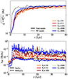 |
Fig. 8. RMS value of the transverse component of the magnetic field (top) and values of the resistivity (bottom) over time for model s10eEr1 reproduced with different resolutions. The maximum and average values of the resistivity are calculated over a rectangular box of sizes Lx × 2a centered on y = 0. |
The reconnecting magnetic flux and the associated reconnection rate shown in Fig. 9 provide a more detailed picture. Results obtained with Nx ≳ 2000 are quantitatively in agreement in terms of the amount of magnetic field reconnected by the t = 40Lu/c mark and the corresponding reconnection rate. However, for Nx = 4096, we obtained a faster and steadier reconnection, reaching the PIC saturation level by t ≃ 30. At the lowest resolution (Nx = 256), the reconnection reaches a halt after the initial fragmentation and merging of the first plasmoids around t ≃ 20Lu/c, at which point the two last magnetic islands remain unmerged for the rest of the simulations and the reconnected magnetic flux stalls. At twice the resolution (Nx = 512), the increase in reconnected flux in the first half of the simulation is not significantly impacted, as shown also by the similar reconnection rate of ≃0.05. However, with 512 points along the x-direction, the model is able to continue the merging of the last large magnetic islands and approach the expected saturation level. Overall, the resulting reconnection rates are qualitatively similar among models at different resolutions, with simulations running on the coarser grids showing a decrease by at most a factor ∼2 in the first stages of the reconnection event.
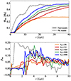 |
Fig. 9. Reconnected magnetic flux (top) and reconnection rate (bottom) over time for the same models as Fig. 8. |
4.2. Initial upstream density
The effective resistivity expressed in Eq. (14) is completely defined by the dynamic state of the plasma and the characteristic length scale,  . However, the initial choice of upstream density, ρ0, can, in principle, have a direct impact on the properties of magnetic dissipation, since the effective resistivity scales as ηeff ∝ ρ−1. To quantify the impact of this dependence, we reproduced model s10eEr1 with a value of ρ0 decreased and increased by a factor 10 (models s10eEr01 and s10eEr10, respectively). Changing this parameter modifies not only the magnitude of the magnetic dissipation, but also the intensity of the upstream magnetic field
  (for a fixed magnetization).
The evolution of the RMS reconnected magnetic field, By (measured in units of B0), appears to be rather insensitive to the variation in ρ0 during the initial exponential growth phase (top panel of Fig. 10). This is consistent with the fact that the upstream Alfvén velocity in all these models is the same, since neither σ0 nor β0 have changed. However, models with higher density tend to start the saturation phase earlier and lead to slightly less reconnection for the magnetic field. Similarly to model s10eC5r1, our simulation with high background density did not reach its conclusion, as a generally much lower value of the resistivity decreases the numerical stability of the code. The temporal profiles of the maximum value assumed by the effective resistivity (bottom panel of Fig. 10) show how this quantity scales indeed with B0/ρ0. The average resistivity along the current sheet shows instead some deviations from such scaling behavior, with again higher densities being associated with even lower resistivities. A similar dependence on ρ0 can be found by looking at the reconnected magnetic flux (Fig. 11), with the least and the most dense cases delivering the fastest and slowest growth of Φrec, respectively. While the differences between the two less dense models (s10eEr01 and s10eEd0r1) do not exceed the level of 10% by the time the two last plasmoids are fully formed (t ≃ 7), the highest density case presents a systematically slower increase of reconnected flux, which directly impacts the corresponding reconnection rates (bottom panel), with βrec ranging from about ∼0.085 (model s10eEr10) to ≃0.11 (model s10eEr01).
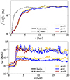 |
Fig. 10. RMS value of the transverse component of the magnetic field (top) and values of the resistivity (bottom) over time for models s10eEr10, s10eEr1, and s10eEr01. The maximum and average values of the resistivity are calculated over a rectangular box of sizes Lx × 2a centered on y = 0. |
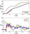 |
Fig. 11. Reconnected magnetic flux (top) and reconnection rate (bottom) over time for the same models as Fig. 10. |
4.3. Initial magnetization
We go on to analyze the role played by the upstream magnetization σ0 in determining the reconnection dynamics by considering two lower values of initial magnetization in addition to the previously discussed benchmark, namely, σ0 ∈ {1, 4, 10}. For these setups, we produced ResRMHD models with effective resistivity as well as the corresponding PIC simulations. Our chosen values for σ0 imply an asymptotic magnetic field B0 ∈ {1, 2, 3.16} and an upstream Alfvén velocity of cA, 0 ∈ {0.887, 0.704, 0.945}, respectively. Both the kinetic and fluid models exhibit similar trends with varying magnetization, with a slower growth of the RMS By field for lower values of σ0 (Fig. 12). This is consistent with the expectation that the dynamic time scale of reconnection in the linear phase of the ideal tearing regime should scale with the Alfvén crossing time, τA = Lu/cA, 0 (Del Zanna et al. 2016). A lower magnetization leads also to a lower saturation of the transverse magnetic field By, an effect that is more pronounced in model s1eEr1. The evolution of the resistivity presents a similar dilation of the dynamic time scale of the reconnection event (bottom panel of Fig. 12). Both the average and maximum values of ηeff are also consistent among different models once they are normalized by B0/ρ0, which is a further confirmation of the scaling behavior of ηeff with the upstream magnetic field and plasma density.
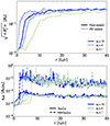 |
Fig. 12. RMS value of the transverse component of the magnetic field (top) and values of the resistivity (bottom) over time for models s10eEr1, s4eEr1, and s1eEr1. The maximum and average values of the resistivity are calculated over a rectangular box of sizes Lx × 2a centered on y = 0. |
The evolution over time of the reconnected magnetic flux in Fig. 13 clearly shows that our ResRMHD models have a systematic initial delay due to the initial linear phase of the tearing instability, whose duration increases for lower magnetizations. This is reflected in the current sheet fragmentation into smaller plasmoids occurring at later times for smaller values of σ0. The PIC models do not experience any such delay for decreasing magnetizations, but have a similar decrease in the growth of the reconnected flux. The corresponding reconnection rates confirm that our ResRMHD models with effective resistivity lead to reconnection events with efficiency in quantitative agreement with PIC models, corroborating the results presented in Sect. 3.1. Moreover, the reconnection rate after the initial transient does not appear to be overly dependent on the magnetization (bottom panel of Fig. 13). This is to be expected when considering that lower values of sigma lead not only to a slower increase of the reconnected flux, but also lower Alfvén speeds.
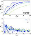 |
Fig. 13. Reconnected magnetic flux (top) and reconnection rate (bottom) over time for the same models as Fig. 12. |
4.4. Reconnection rate trends
Next, we can compare the reconnection rates obtained in this work in a more quantitative way, namely, by computing a representative time average for each one of simulations we performed. To exclude the initial transient and the later stage close to the saturation, we calculated the average in the time interval where the reconnected magnetic flux is between 30% and 60% of its maximum value. We applied this procedure to a larger set of simulation with respect to the ResRMHD and PIC models presented in the previous sections, which leads to the scatter plot of ⟨βrec⟩ against the spatial resolution, shown in Fig. 14.
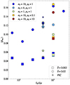 |
Fig. 14. Average reconnection rate against resolution for the ResRMHD models with effective resistivity (circles and squares) and the PIC models (stars). Small and large stars refer to PIC models having initial perturbations with amplitude 0.001 and 0.05, respectively. |
The dependence on the grid resolution is evident for both models s10eEr1 and s10eEd0r1, as the reconnection rate increases by up to a factor ∼1.5 between the most coarse grid and the reference cases discussed in Sect. 3.1. However, the run with Nx = 8192 for model s10eEd0r1 suggests that there should be no further quantitative deviations for higher resolutions and that indeed our measured rates are numerically converged. All fluid models produce reconnection rates within the same order of magnitude of the kinetic simulations, with the limit case of  being in quantitative agreement with the corresponding PIC realizations. We assessed the variance of the rates produced by the kinetic models by performing an additional set of simulations with the same range of values for σ0, but with weaker initial perturbations (ϵ = 0.001 rather than 0.05); these are represented by the smaller stars in Fig. 14 and deviate from the runs with stronger perturbation by 10−20% at most. The same trend with magnetization is reproduced by all PIC and ResRMHD models, namely, there is little variance seen for different values of σ0. Simulations with
  and Nx = 4096 appear to be an exception, with the reconnection rate increasing by up to 60% with higher magnetizations. The PIC models with σ0 = 1 also deviate from the other kinetic simulations, this time by a factor of ∼2. Changing the upstream plasma density impacts the corresponding reconnection rate for both values of the plasma skin depth parameter explored. A variation over two orders of magnitude in terms of ρ0 introduces a deviation in the average reconnection rate of Δ⟨βrec⟩ between ∼0.02 and ∼0.04. Model s10eEr10 (red square) appears to have larger ⟨βrec⟩ than expected from the discussion presented in Sect. 4.2. This is likely an artifact that is due to the short duration of the simulation, which prevents a more significant decrease in the reconnection rate over time.
5. Conclusions
We presented a series of ResRMHD numerical simulations of magnetic reconnection that address the gap between fluid and kinetic models of astrophysical plasmas by using, for the first time, an effective resistivity formulation derived from recent first-principle PIC models. We adapted the closure obtained by Selvi et al. (2023) to express the resistivity in terms of fluid quantities and known constants, which allows us to constrain the dissipation properties of the plasma by its local state and the characteristic length scales of the reconnecting current sheet.
All our ResRMHD models with effective resistivity lead to a fast reconnection of the initial magnetic field, with a quick fragmentation of the current sheet into plasmoids and the saturation into a large magnetic island within ≃20 dynamical timescales. The evolution of the current sheet is in good agreement among the fluid and kinetic models, which confirms the capability of the effective resistivity to capture the intrinsically collisionless nature of magnetic reconnection. To capture the onset of the ideal tearing instability on dynamical timescales, constant resistivity models require very low values of η; therefore, we need sufficiently high grid resolutions to describe the smaller dissipation length scale of the simulation. On the other hand, the effective resistivity formulation allows us to retrieve fast reconnections, even at a very modest resolution. This is due to the fact that the enhanced magnetic dissipation within the current sheet induces strong reconnection without requiring the tearing instability to thin the current sheet’s width. Future works will be aimed at making a more thorough comparison between the effective resistivity models and the dynamics of relativistic reconnection at high Lundquist numbers. This will require higher resolutions and will benefit from recently developed higher order schemes for RMHD and ResRMHD models Berta et al. (2024), Mignone et al. (2024).
While both strong non-ideal electric fields and velocity gradients a priori can contribute to enhance the resistivity (see Eq. 14), the former contribution dominates in the regions with the highest dissipation. This is because it is at first order in the dimensionless plasma skin-depth parameter,  , rather than second. This suggests that our effective resistivity formulation might be simplified even more to include exclusively the non-ideal electric field, especially when applied to astrophysical systems with larger size than an isolated current sheet (e.g., a relativistic jet or a black hole magnetosphere). Such formulation would be similar to the one presented in Ripperda et al. (2019b), where the resistivity was taken to be proportional to the local current density, but with the coupling constant (
 ) representing the “effective” plasma skin depth that the fluid system is allowed to see.
The value of this coupling constant can have a significant impact on the resulting reconnection dynamics. Taking  equal to the plasma skin depth in the current sheet leads to a fragmentation into plasmoids and merging phase that qualitatively resembles both PIC models and constant resistivity ResRMHD simulations. The corresponding reconnection rates are much higher than in the case with constant magnetic dissipation, but slightly lower than the kinetic counterparts. On the other hand, a plasma skin depth that is ten times greater and matches the upstream conditions of the problem reproduces the diagnostics obtained by first-principles simulations in a more quantitative way; however, the underlying plasmoid dynamics deviates qualitatively from the standard scenario, as the increased dissipation leads to the formation of hot, rarefied cavities between large magnetic islands that prevent the production of smaller plasmoids connected by thinning reconnecting regions. These differences are likely to have a significant impact on how particles are accelerated during the reconnection event, which we will assess in an upcoming work. The choice of the numerical value for the
  parameter becomes less evident for problems where the current sheet is not already present from the beginning. In our reconnection models, we are, in practice, imposing a characteristic mass density unit that makes this parameter equal to the actual current sheet skin depth set by the corresponding PIC model. Since a different value of
  is likely to affect the formation of current sheets themselves (e.g., during the merge of two flux tubes), setting its value a priori requires more dedicated comparative studies between PIC and ResRMHD models. Future works will have to explore the dependence of our effective resistivity model on
  more thoroughly for different initial pressure-balanced equilibria (e.g., with constant density or different temperatures), as well as for merging flux tubes (Ripperda et al. 2019a).
Our simulations show that a higher background density tends to weaken the reconnection and decrease the reconnection rate, as the mean resistivity within the current sheet is lowered by a factor of a few. This is a direct consequence of the prescription we used for ηeff being inversely proportional to the plasma density. We also verified that lower magnetizations produce slower reconnection events and lower reconnection rates (which is also expected in the constant resistivity case), with the mean resistivity scaling with the quantity B0/ρ0.
The fast reconnection of magnetic flux occurring in our ResRMHD simulations is reflected by high reconnection rates (between ∼0.05 and ∼0.2). These measurements are not only an order of magnitude larger than those produced in the constant resistivity case, but they are also in quantitative agreement with the corresponding PIC models. This result showcases the potential of the effective resistivity formalism to reproduce (within the standard ResRMHD framework) the results of first-principles kinetic models. This enables a more accurate modeling of large-scale astrophysical systems, where reconnection is expected to occur. Accretion flows on black holes would be a prime example of such an application, in particular in the so-called MAD state Tchekhovskoy et al. (2011). Since the amount of dissipation regulates the magnetic flux available at the event horizon, the inclusion of an effective resistivity might change the properties of the saturated state. Moreover, a faster reconnection dynamics could profoundly impact the formation of possible particle acceleration sites in relativistic jets launched by newly formed compact objects (Mattia et al. 2023, 2024). However, it should be noted that the prospects of resolving the actual skin depth of current sheets in large-scale astrophysical models are quite poor, given the large scale separation involved. The application of our formulation to models of accreting compact objects or relativistic jets will thus require a compromise, namely, adopting a much larger “effective” skin depth; otherwise, the low resulting resistivity would simply have no dynamical effects against the grid numerical dissipation (in addition to it leading to numerical instabilities). This approach would be keen to the one adopted successfully by large scale GR-PIC models of relativistic magnetospheres (Crinquand et al. 2021, 2022; El Mellah et al. 2022), which settle for a similar trade-off for the plasma skin depth. Given this similarity, a closer comparison between such models and GRMHD simulations with effective resistivity might provide important insights on the dynamics of magnetic dissipation in a regime of strong gravity.
Although our results show a remarkable agreement between fluid and kinetic models, it should be noted that the derivation of Eq. (14) relies on some strong assumptions. In particular, we introduced the current density (and, therefore, the electric field) in the expression for ηeff to more directly tie the enhanced dissipation to the reconnection layer; however, our derivation should be more rigorously verified to fully characterize the impact of non-collisional effects on magnetic dissipation within the ResRMHD framework. Moreover, the “kinetic” formulation of the effective resistivity presented by Selvi et al. (2023) has been obtained in the absence of a guide field and for a electron-positron plasma; meanwhile, it remains unclear how the scenario would change with different magnetic field configurations or in the presence of ions. Another limitation comes from the fact that the effective resistivity measurements were performed specifically in the X-points of the reconnecting current sheet. Although they are undoubtedly the most relevant locations to study, further investigations with fully kinetic models of relativistic reconnection are required to assess the general character of the proposed formulation.
Furthermore, our 2D results capture the main properties of how magnetic field is dissipated and particles are accelerated during a reconnection event, but they should be further tested in 3D to verify the extent of the validity of the prescription we used. Finally, it should be noted that Eqs. (7) and (14) assume the current sheet to be locally aligned with the x-axis, as the only velocity gradients appearing are those along the transverse direction, y. This means that our prescription is likely to underestimate the contribution to the effective resistivity of the fluid velocity gradients, since the non-linear stage of the tearing instability leads to the formation of secondary current sheets perpendicular to the x-axis between merging plasmoids. This aspect might be relevant when quantifying the efficiency of particle acceleration when using the effective resistivity formulation. A more consistent approach would require the identification of the local orientation of the current sheet to correctly include the velocity gradients that are perpendicular to that direction. We leave such an improvement to a follow-up study.
Acknowledgments
We thank the anonymous referee for improving this work with useful comments and suggestions. M.B. would like to thank Bart Ripperda, Sasha Philippov, Niccolò Bucciantini, and Emanuele Papini for useful discussions. This project has received funding from the European Union’s Horizon Europe research and innovation programme under the Marie Skłodowska-Curie grant agreement No. 101064953 (GR-PLUTO). B.C. and E.F. are supported by the European Research Council (ERC) under the European Union’s Horizon 2020 research and innovation program (Grant Agreement No. 863412). L.D.Z. acknowledges support from the ICSC–Centro Nazionale di Ricerca in High-Performance Computing; Big Data and Quantum Computing, funded by European Union – NextGenerationEU. This work has received funding from the European High Performance Computing Joint Undertaking (JU) and Belgium, Czech Republic, France, Germany, Greece, Italy, Norway, and Spain under grant agreement No. 101093441. This paper is also supported by the Fondazione ICSC, Spoke 3 Astrophysics and Cosmos Observations, National Recovery and Resilience Plan (Piano Nazionale di Ripresa e Resilienza, PNRR) Project ID CN_00000013 “Italian Research Center on High-Performance Computing, Big Data and Quantum Computing” funded by MUR Missione 4 Componente 2 Investimento 1.4: Potenziamento strutture di ricerca e creazione di “campioni nazionali di R&S (M4C2-19)” – Next Generation EU (NGEU). Computational resources on the OCCAM cluster (https://c3s.unito.it/index.php/super-computer) were provided by the Centro di Competenza sul Calcolo Scientifico (C3S) of the University of Torino. We also acknowledge CINECA for the availability of high performance computing resources and support on the LEONARDO supercomputer (https://leonardo-supercomputer.cineca.eu/) through a CINECA-INFN agreement, providing the allocations INF23_teongrav and INF24_teongrav. Computing resources for performing the PIC simulations were provided by TGCC under the allocation A0150407669 made by GENCI. The figures presented in this paper were generated using the PyPLUTO (https://github.com/GiMattia/PyPLUTO) package (Mattia et al., in prep.) while all the line colors have been checked through a color blindness simulator (https://www.color-blindness.com/coblis-color-blindness-simulator/).
References
- Berta, V., Mignone, A., Bugli, M., & Mattia, G. 2024, J. Comput. Phys., 499, 112701 [Google Scholar]
- Birdsall, C. K., & Langdon, A. B. 1991, Plasma Physics via Computer Simulation (New York: McGraw-Hill) [CrossRef] [Google Scholar]
- Bucciantini, N., & Del Zanna, L. 2013, MNRAS, 428, 71 [NASA ADS] [CrossRef] [Google Scholar]
- Castro, M., Costa, B., & Don, W. S. 2011, J. Comput. Phys., 230, 1766 [Google Scholar]
- Cerutti, B., & Werner, G. 2019, Astrophysics Source Code Library [record ascl:1911.012] [Google Scholar]
- Cerutti, B., Uzdensky, D. A., & Begelman, M. C. 2012a, ApJ, 746, 148 [Google Scholar]
- Cerutti, B., Werner, G. R., Uzdensky, D. A., & Begelman, M. C. 2012b, ApJ, 754, L33 [NASA ADS] [CrossRef] [Google Scholar]
- Cerutti, B., Werner, G. R., Uzdensky, D. A., & Begelman, M. C. 2013, ApJ, 770, 147 [Google Scholar]
- Crinquand, B., Cerutti, B., Dubus, G., Parfrey, K., & Philippov, A. 2021, A&A, 650, A163 [NASA ADS] [CrossRef] [EDP Sciences] [Google Scholar]
- Crinquand, B., Cerutti, B., Dubus, G., Parfrey, K., & Philippov, A. 2022, Phys. Rev. Lett., 129, 205101 [NASA ADS] [CrossRef] [Google Scholar]
- Del Zanna, L., & Bucciantini, N. 2018, MNRAS, 479, 657 [NASA ADS] [Google Scholar]
- Del Zanna, L., Papini, E., Landi, S., Bugli, M., & Bucciantini, N. 2016, MNRAS, 460, 3753 [Google Scholar]
- El Mellah, I., Cerutti, B., Crinquand, B., & Parfrey, K. 2022, A&A, 663, A169 [NASA ADS] [CrossRef] [EDP Sciences] [Google Scholar]
- Giannios, D. 2013, MNRAS, 431, 355 [NASA ADS] [CrossRef] [Google Scholar]
- Hesse, M., & Zenitani, S. 2007, Phys. Plasmas, 14, 112102 [NASA ADS] [CrossRef] [Google Scholar]
- Komissarov, S. 2007, MNRAS, 382, 995 [CrossRef] [Google Scholar]
- Komissarov, S., & Phillips, D. 2024, ArXiv e-prints [arXiv:2409.03637] [Google Scholar]
- Landi, S., Del Zanna, L., Papini, E., Pucci, F., & Velli, M. 2015, ApJ, 806, 131 [NASA ADS] [CrossRef] [Google Scholar]
- Londrillo, P., & del Zanna, L. 2004, J. Comput. Phys., 195, 17 [NASA ADS] [CrossRef] [Google Scholar]
- Lyubarskii, Y. E. 1996, A&A, 311, 172 [NASA ADS] [Google Scholar]
- Mahlmann, J. F., Philippov, A. A., Levinson, A., Spitkovsky, A., & Hakobyan, H. 2022, ApJ, 932, L20 [NASA ADS] [CrossRef] [Google Scholar]
- Mattia, G., Del Zanna, L., Bugli, M., et al. 2023, A&A, 679, A49 [NASA ADS] [CrossRef] [EDP Sciences] [Google Scholar]
- Mattia, G., Del Zanna, L., Pavan, A., & Ciolfi, R. 2024, A&A, 691, A105 [NASA ADS] [CrossRef] [EDP Sciences] [Google Scholar]
- McKinney, J. C., & Uzdensky, D. A. 2012, MNRAS, 419, 573 [Google Scholar]
- Mignone, A., Bodo, G., Massaglia, S., et al. 2007, ApJS, 170, 228 [Google Scholar]
- Mignone, A., Mattia, G., Bodo, G., & Del Zanna, L. 2019, MNRAS, 486, 4252 [NASA ADS] [CrossRef] [Google Scholar]
- Mignone, A., Berta, V., Rossazza, M., et al. 2024, MNRAS, 533, 1670 [CrossRef] [Google Scholar]
- Most, E. R., & Philippov, A. A. 2023, Phys. Rev. Lett., 130, 245201 [Google Scholar]
- Nalewajko, K., Uzdensky, D. A., Cerutti, B., Werner, G. R., & Begelman, M. C. 2015, ApJ, 815, 101 [NASA ADS] [CrossRef] [Google Scholar]
- Nathanail, A., Mpisketzis, V., Porth, O., Fromm, C. M., & Rezzolla, L. 2022, MNRAS, 513, 4267 [NASA ADS] [CrossRef] [Google Scholar]
- Olmi, B., Del Zanna, L., Amato, E., Bucciantini, N., & Mignone, A. 2016, J. Plasma Phys., 82, 635820601 [NASA ADS] [CrossRef] [Google Scholar]
- Palenzuela, C., Lehner, L., Reula, O., & Rezzolla, L. 2009, MNRAS, 394, 1727 [Google Scholar]
- Pareschi, L., & Russo, G. 2005, J. Sci. Comput., 25, 129 [MathSciNet] [Google Scholar]
- Petropoulou, M., Giannios, D., & Sironi, L. 2016, MNRAS, 462, 3325 [NASA ADS] [CrossRef] [Google Scholar]
- Pucci, F., & Velli, M. 2014, ApJ, 780, L19 [Google Scholar]
- Puzzoni, E., Mignone, A., & Bodo, G. 2021, MNRAS, 508, 2771 [CrossRef] [Google Scholar]
- Qian, Q., Fendt, C., Noble, S., & Bugli, M. 2017, ApJ, 834, 29 [Google Scholar]
- Ripperda, B., Bacchini, F., Porth, O., et al. 2019a, ApJS, 244, 10 [NASA ADS] [CrossRef] [Google Scholar]
- Ripperda, B., Porth, O., Sironi, L., & Keppens, R. 2019b, MNRAS, 485, 299 [CrossRef] [Google Scholar]
- Ripperda, B., Liska, M., Chatterjee, K., et al. 2022, ApJ, 924, L32 [NASA ADS] [CrossRef] [Google Scholar]
- Selvi, S., Porth, O., Ripperda, B., et al. 2023, ApJ, 950, 169 [NASA ADS] [CrossRef] [Google Scholar]
- Sironi, L. 2022, Phys. Rev. Lett., 128, 145102 [CrossRef] [Google Scholar]
- Sironi, L., & Spitkovsky, A. 2014, ApJ, 783, L21 [NASA ADS] [CrossRef] [Google Scholar]
- Speiser, T. W. 1970, Planet. Space Sci., 18, 613 [NASA ADS] [CrossRef] [Google Scholar]
- Tchekhovskoy, A., Narayan, R., & McKinney, J. C. 2011, MNRAS, 418, L79 [NASA ADS] [CrossRef] [Google Scholar]
- Tomei, N., Del Zanna, L., Bugli, M., & Bucciantini, N. 2020, MNRAS, 491, 2346 [Google Scholar]
- Uzdensky, D. A., & Spitkovsky, A. 2014, ApJ, 780, 3 [NASA ADS] [Google Scholar]
- Vos, J. T., Olivares, H., Cerutti, B., & Mościbrodzka, M. 2024, MNRAS, 531, 1554 [NASA ADS] [CrossRef] [Google Scholar]
- Watanabe, N., & Yokoyama, T. 2006, ApJ, 647, L123 [Google Scholar]
- Werner, G. R., Uzdensky, D. A., Cerutti, B., Nalewajko, K., & Begelman, M. C. 2016, ApJ, 816, L8 [Google Scholar]
- Yee, K. 1966, IEEE Trans. Antennas Propag., 14, 302 [Google Scholar]
- Zanotti, O., & Dumbser, M. 2011, MNRAS, 418, 1004 [NASA ADS] [CrossRef] [Google Scholar]
- Zenitani, S., & Hoshino, M. 2001, ApJ, 562, L63 [NASA ADS] [CrossRef] [Google Scholar]
- Zenitani, S., Hesse, M., & Klimas, A. 2010, ApJ, 716, L214 [NASA ADS] [CrossRef] [Google Scholar]
- Zhang, B., & Yan, H. 2011, ApJ, 726, 90 [Google Scholar]
Appendix A: Numerical benchmarks
Here, we present a series of tests designed to validate our implementation of the effective resistivity within the ResRMHD module of the PLUTO code.
A.1. Uniform stationary resistive plasma
Using our prescription for the effective resistivity in Eq. 10 we can express Ampère’s law as
![Mathematical equation: $$ \begin{aligned} \partial _t \boldsymbol{E} - \boldsymbol{\nabla } \times \boldsymbol{B} = -\Gamma \frac{|J_0|}{\sqrt{E_0^2 + e_z^2}} [\boldsymbol{E} + \boldsymbol{v} \times \boldsymbol{B} - (\boldsymbol{E} \cdot \boldsymbol{v})\boldsymbol{v}] - q\boldsymbol{v}. \end{aligned} $$](/articles/aa/full_html/2025/01/aa52277-24/aa52277-24-eq68.gif) (A.1)
(A.1)
If we now assume to have a stationary, unmagnetized, and uniform plasma with

we can reduce Eq. A.1 to
 (A.2)
(A.2)
This equation requires only the integration of the z component of the electric field, since we can take the other two as proportional to Ez (i.e., Ex, y = αx, yEz) and obtain the exact same differential equation for the electric field, namely,
 (A.3)
(A.3)
The proportionality factors for Ex, y are simply retrieved from the initial condition by requiring Ex, y(t)/Ex, y(0) = Ez(t)/Ex(0). By integrating Eq. A.3 in time, we can finally obtain the analytical solution
where τ = Ez(0)/|J0| is the timescale required for the electric field to be completely dissipated. We note that such solution differs substantially from the case with constant resistivity η0, which would instead lead to an exponential decay of the electric field, according to ∂tE = −η0−1E.
The left panel of Fig. A.1 shows the results of a 1d simulation of such configuration using our effective resistivity prescription and an initial uniform electric field given by E = (3, 2, −1) and setting |J0| = 1. The field correctly decays linearly with time, completely vanishing at t = τ = 1. The effective resistivity starts with a value equal to Ez/|J0| = 1 and decays proportionally with the electric field, reaching the minimun floor value ηfloor = 10−6 at t = 1 (right panel of Fig. A.1).
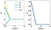 |
Fig. A.1. Electric field decay (left panel) and effective resistivity (right) over time for the uniform stationary resistive test with vanishing velocity gradients. The analytical solution is represented with the blue dashed line. |
We further tested our implementation of the effective resistivity by extending the previous test to non-vanishing velocity gradients, namely, ∂yvy ≠ 0. In this case, Ampère’s law takes the form of
 (A.4)
(A.4)
which can be reduced to a single equation for the z component of the electric field as it was for Eq. A.1. Equation A.4 can be then integrated to obtain
 (A.5)
(A.5)
which can be solved numerically once the integration constant K is set by the initial conditions.
The left panel of Fig. A.2 shows both the field described by Eq. A.5 and the solution obtained by the PLUTO code with J0 = 1, E0 = 0.5, and the same initial electric field as the previous test. Also in this case the code’s calculation agrees with the analytic solution, which leads to the complete dissipation of the electric field by t ≃ 4. However, its decay is no longer linear but rather exponential-like, as the non-vanishing E0 introduces a minimum constant resistivity acting during the whole evolution of the system. This can be seen in the evolution over time of the resistivity (right panel of Fig. A.2), which starts from an initial value  and then decays down to the terminal value E0/|J0| = 0.5.
A.2. 1D self-similar current sheet
As second test for our implementation of the effective resistivity, we considered the self-similar dissipation of a 1D current sheet (Komissarov 2007). While this problem has become a standard numerical test for resistive RMHD codes, we use it here as a benchmark to characterize the action of the effective resistivity in a more realistic and physically motivated setup.
In the limit of infinite resistivity and thermal pressure only the magnetic field evolves, with the induction equation being the only one that needs to be solved. In this resistive regime, the magnetic field evolves in time according to
 (A.6)
(A.6)
We start our simulations at the instant t = 1 imposing ρ = 1, p = 50, B0 = 1, and B = (Bx(y, t = 1),0, 0). Along with the test using the effective resistivity prescription, we also run a benchmark with constant resistivity η0 = 0.1 which will serve as reference. The same value is used in Eq. A.6 to set identical initial conditions for the effective resistivity case. The 1D computational domain covers with Ny = 4096 grid points a transversal slice of a current sheet with y ∈ [ − 20, 20]. As for the previous tests, we used RK3 timestepping, MP5 reconstruction, and we set |J0| = 1.
The top panel of Fig. A.3 shows the evolution of the current sheet when using a constant value for the resistivity η = 0.1, which reproduces the analytical profile described by Eq. A.6 (dotted curves). When we use the effective resistivity prescription (mid panel), there is a localized dissipation of the current sheet closer to its center, with a continuous expanding of the region affected by the magnetic dissipation. The magnetic field relaxes then towards a profile that increases linearly with the domain coordinate x. This behaviour is consistent with the actual evolution of η (bottom panel), which starts from its imposed floor value ηfloor = 10−6. It then increases to values larger than 0.1 by t = 1.5 but only within Δx ≃ 1 from the current sheet’s center, whereas it remains weaker by at least two orders of magnitude for further distances. As time progresses, the resistivity profile becomes flatter over a larger region, while also decreasing in amplitude and approaching a mean value within the current sheet of ∼0.01 by t ≃ 3.
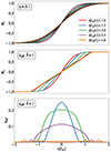 |
Fig. A.3. 1D self-similar current sheet. Top panel: Spatial profiles of By for a constant resistivity at different times. The analytical solution given by Eq. A.6 is indicated with black dotted lines. Mid panel: Same as the top panel, but using an effective resistivity. Bottom panel: Spatial profiles of effective resistivity at different times. |
All Tables
ResRMHD and PIC models and their parameters: upstream “cold” magnetization, Alfvèn speed, resistivity, effective plasma skin depth, upstream density, and magnetic field.
All Figures
|
Fig. 1. Spatial profiles of (from top to bottom) mass density, ratio of comoving electric field over current density ez/jz, and ez for the kinetic model s10pic at t ≃ 2.4. The density is normalized by the upstream value, ρ0, the electric field by the upstream magnetic field, B0, and the current density by |
| In the text | |
|
Fig. 2. Space-time diagrams of different quantities at the center of the current sheet (y = 0) over time for the ResRMHD model s10eEr1. From top left to bottom right: Rest-mass density ρ, effective resistivity ηeff, z-component of the electric field in the fluid frame ez, and Lorentz invariant B2 − E2. The white dotted lines indicate the instant where the profiles in Fig. 3 are shown. |
| In the text | |
|
Fig. 3. Spatial profiles of (from top to bottom) the rest-mass density, ρ, the effective resistivity, ηeff, the z-component of the electric field in the fluid frame, ez, the Lorentz invariant, B2 − E2, with the contours of the vector potential, Az, and the temperature for the ResRMHD model s10eEr1 at t = 6.3. |
| In the text | |
|
Fig. 4. Same as Fig. 2, but for the ResRMHD model s10eEd0r1. The white dotted lines indicate the instant at which the profiles in Fig. 5 are shown. |
| In the text | |
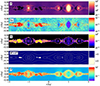 |
Fig. 5. Same as Fig. 3, but for the ResRMHD model s10eEd0r1 at t = 4.5. |
| In the text | |
|
Fig. 6. RMS value of the transverse component of the magnetic field (top) and values of the resistivity (bottom) over time for ResRMHD models s10eEr1 (blue curve), s10eEd0r1 (red), models with constant resistivity (green, yellow, light purple, and purple), and model s10pic (dotted). The maximum and average values of the resistivity are calculated over a rectangular box of sizes Lx × 2a centered on y = 0. |
| In the text | |
|
Fig. 7. Reconnected magnetic flux (top) and reconnection rate (bottom) over time for the same models as those in Fig. 6. |
| In the text | |
|
Fig. 8. RMS value of the transverse component of the magnetic field (top) and values of the resistivity (bottom) over time for model s10eEr1 reproduced with different resolutions. The maximum and average values of the resistivity are calculated over a rectangular box of sizes Lx × 2a centered on y = 0. |
| In the text | |
|
Fig. 9. Reconnected magnetic flux (top) and reconnection rate (bottom) over time for the same models as Fig. 8. |
| In the text | |
|
Fig. 10. RMS value of the transverse component of the magnetic field (top) and values of the resistivity (bottom) over time for models s10eEr10, s10eEr1, and s10eEr01. The maximum and average values of the resistivity are calculated over a rectangular box of sizes Lx × 2a centered on y = 0. |
| In the text | |
|
Fig. 11. Reconnected magnetic flux (top) and reconnection rate (bottom) over time for the same models as Fig. 10. |
| In the text | |
|
Fig. 12. RMS value of the transverse component of the magnetic field (top) and values of the resistivity (bottom) over time for models s10eEr1, s4eEr1, and s1eEr1. The maximum and average values of the resistivity are calculated over a rectangular box of sizes Lx × 2a centered on y = 0. |
| In the text | |
|
Fig. 13. Reconnected magnetic flux (top) and reconnection rate (bottom) over time for the same models as Fig. 12. |
| In the text | |
|
Fig. 14. Average reconnection rate against resolution for the ResRMHD models with effective resistivity (circles and squares) and the PIC models (stars). Small and large stars refer to PIC models having initial perturbations with amplitude 0.001 and 0.05, respectively. |
| In the text | |
|
Fig. A.1. Electric field decay (left panel) and effective resistivity (right) over time for the uniform stationary resistive test with vanishing velocity gradients. The analytical solution is represented with the blue dashed line. |
| In the text | |
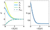 |
Fig. A.2. Same as Fig. A.1 but for the non-vanishing velocity gradients case. |
| In the text | |
|
Fig. A.3. 1D self-similar current sheet. Top panel: Spatial profiles of By for a constant resistivity at different times. The analytical solution given by Eq. A.6 is indicated with black dotted lines. Mid panel: Same as the top panel, but using an effective resistivity. Bottom panel: Spatial profiles of effective resistivity at different times. |
| In the text | |
Current usage metrics show cumulative count of Article Views (full-text article views including HTML views, PDF and ePub downloads, according to the available data) and Abstracts Views on Vision4Press platform.
Data correspond to usage on the plateform after 2015. The current usage metrics is available 48-96 hours after online publication and is updated daily on week days.
Initial download of the metrics may take a while.