| Issue |
A&A
Volume 679, November 2023
|
|
|---|---|---|
| Article Number | A49 | |
| Number of page(s) | 17 | |
| Section | Astrophysical processes | |
| DOI | https://doi.org/10.1051/0004-6361/202347126 | |
| Published online | 01 November 2023 | |
Resistive relativistic MHD simulations of astrophysical jets⋆
1
INFN, Sezione di Firenze, Via G. Sansone 1, 50019 Sesto Fiorentino, Italy
e-mail: This email address is being protected from spambots. You need JavaScript enabled to view it.
2
Dipartimento di Fisica e Astronomia, Università di Firenze, Via G. Sansone 1, 50019 Sesto Fiorentino, Italy
3
INAF, Osservatorio Astrofisico di Arcetri, Largo E. Fermi 5, 50125 Firenze, Italy
4
Dipartimento di Fisica, Università di Torino, Via P. Giuria 1, 10125 Torino, Italy
5
Université Paris-Saclay, Université Paris Cité, CEA, CNRS, AIM, 91191, Gif-sur-Yvette, France
6
INFN, Sezione di Torino, Via P. Giuria 1, 10125 Torino, Italy
7
Dipartimento di Fisica e Astronomia, Università di Padova, Via F. Marzolo 8, 35131 Padova, Italy
8
INAF, Osservatorio Astronomico di Padova, Vicolo dell’Osservatorio 5, 35122 Padova, Italy
9
INFN, Sezione di Padova, Via F. Marzolo 8, 35131 Padova, Italy
10
INAF, Osservatorio Astrofisico di Torino, Strada Osservatorio 20, 10025 Pino Torinese, Italy
Received:
8
June
2023
Accepted:
16
August
2023
Abstract
Aims. The main goal of the present paper is to provide the first systematic numerical study of the propagation of astrophysical relativistic jets, in the context of high-resolution, shock-capturing Resistive Relativistic MagnetoHydroDynamic (RRMHD) simulations. We aim to investigate different values and models for the plasma resistivity coefficient, and to assess their impact on the level of turbulence, the formation of current sheets and reconnection plasmoids, the electromagnetic energy content, and the dissipated power.
Methods. We used the PLUTO code for simulations and we assumed an axisymmetric setup for the jets, endowed with both poloidal and toroidal magnetic fields, and propagating in a uniform magnetized medium. The gas was assumed to be characterized by a realistic, Synge-like equation of state (the Taub equation), appropriate for such astrophysical jets. The Taub equation was combined here for the first time with the implicit-explicit Runge-Kutta time-stepping procedure, as required in RRMHD simulations.
Results. The main result is that turbulence is clearly suppressed for the highest values of resistivity (low Lundquist numbers), current sheets are broader, and plasmoids are barely present, while for low values of resistivity the results are very similar to ideal runs, in which dissipation is purely numerical. We find that recipes employing a variable resistivity based on the advection of a jet tracer or on the assumption of a uniform Lundquist number improve on the use of a constant coefficient and are probably more realistic possible sites for the acceleration of the nonthermal particles that produce the observed high-energy emission, preserving as they do the development of turbulence and of sharp current sheets.
Key words: magnetohydrodynamics (MHD) / magnetic reconnection / relativistic processes / shock waves / galaxies: jets / methods: numerical
The PLUTO code is publicly available. Simulation data will be shared on reasonable request to the corresponding author.
© The Authors 2023
 Open Access article, published by EDP Sciences, under the terms of the Creative Commons Attribution License (https://creativecommons.org/licenses/by/4.0), which permits unrestricted use, distribution, and reproduction in any medium, provided the original work is properly cited.
This article is published in open access under the Subscribe to Open model. This email address is being protected from spambots. You need JavaScript enabled to view it. to support open access publication.
1. Introduction
Astrophysical jets, that is to say supersonic collimated outflows, represent a ubiquitous phenomenon in the Universe, characterizing various classes of celestial sources at very different spatial scales and evolutionary stages. In particular, the interplay of strong gravity, rotation, and the magnetic fields of compact objects can cause the launching of relativistic jets, even with high Lorentz factors, as spectacularly demonstrated by their apparent superluminal motion when propagation is close to the line of sight, and more recently by the imaging of the supermassive black hole that is the inner engine of the kiloparsec-scale jet of M 87 (Event Horizon Telescope Collaboration 2019). Other than in active galactic nuclei (AGN), relativistic outflows and jets are also present in several types of stellar-sized astrophysical bodies, such as the collapsing sources of long gamma-ray bursts (GRBs; Woosley 1993) and pulsar wind nebulae (Weisskopf et al. 2000). Recently we also had the first multi-messenger indication that binary neutron star (BNS) merger events are able to drive relativistic outflows in the form of short GRBs (Abbott et al. 2017). The electromagnetic spectral signature of such objects often features highly nonthermal radiation, mostly synchrotron and inverse Compton processes, due to accelerated relativistic particles (electrons). In the case of AGNs, particles can be accelerated either in the inner engine and advected, or along the jet and at the terminal radio lobes (e.g., Begelman et al. 1984; Blandford et al. 2019). More recently, even protostellar jets have shown similar radiation features (Lee et al. 2018).
Different processes have been invoked in order to explain such particle acceleration in astrophysical sources. In particular, relativistic magnetic (fast) reconnection, in other words the impulsive topological rearrangement of field lines in a magnetically dominated or very hot plasma (Lyutikov & Uzdensky 2003; Lyubarsky 2005; Komissarov et al. 2007; Del Zanna et al. 2016; Ripperda et al. 2019b) is a very general and promising acceleration process, which has been extensively investigated in recent years, especially through particle-in-cell (PIC) simulations (Sironi & Spitkovsky 2014; Cerutti et al. 2014; Comisso & Sironi 2018; Zhang et al. 2021). The precise mechanism regulating the acceleration of particles during the reconnection process, namely the formation of X and O points and the subsequent merging of plasmoids (e.g., Loureiro & Uzdensky 2016), is still debated, as is their impact on the large-scale scenario (e.g., Medina-Torrejón et al. 2023).
Because of the unavoidable numerical resistivity present in every MagnetoHydroDynamic (MHD) simulation (even within the ideal framework), the disentanglement of the effects due to the truncation error from the physical process is a key point in order to understand the role of magnetic reconnection in astrophysical jets. The most critical issue of the ideal approximation (which constrains the electric field to the standard −v × B) is the lack of control over the numerical diffusivity, which becomes strongly susceptible to the grid resolution and numerical algorithms (Núñez-de la Rosa & Munz 2016; Felker & Stone 2018).
It is therefore important to perform numerical simulations of astrophysical plasmas that go beyond the usual assumption of ideal MHD almost invariably employed, especially in the relativistic regime. The simplest possible framework in which the role of a finite plasma conductivity can be investigated is that of the Resistive Relativistic MagnetoHydroDynamic (henceforth Resistive Relativistic MHD or RRMHD) regime, in which the electric field in the coming frame is not vanishing, as in the ideal MHD case, but simply proportional to the local current density through a (scalar for simplicity) resistivity coefficient, η. This way, the electric field in the laboratory frame is allowed to depart from its ideal configuration (which imposes a vanishing component along the magnetic field lines), especially in current sheets, where reconnection events and particle acceleration are expected to take place. Obviously, no current numerical modeling will ever achieve the realistic low values of η typical of collisionless astrophysical plasmas, though it is well known that unresolved, small-scale turbulent fluctuations may act as sources of additional dissipation (see the conclusions for additional comments on sub-grid modeling).
Here we just want to stress that the RRMHD regime makes it possible to single out the regions where resistive effects may be important, by adopting a physically motivated model. This is impossible in numerical ideal MHD, where magnetic dissipation is invariably present at the grid level (due to numerical round-off errors) and no nonideal aspect can be controlled. Moreover, employing an explicit resistivity allows for more meaningful comparisons between models produced with different codes and numerical algorithms, as the uncertainties related to magnetic numerical dissipation are removed. Thus, this approach promotes the reproducibility of jet simulations and strengthens the physical interpretation of their results.
Most of the RRMHD numerical investigations of reconnection, either due to the tearing instability in preexisting current sheets (e.g., Del Zanna et al. 2016), or formed in the process of a turbulent cascade (e.g., Chernoglazov et al. 2021), involve localized portions of plasma and periodic boundary conditions. Other studies assume reconnection induced by current-driven kink instabilities in (periodic) columns of magnetized plasma (Medina-Torrejón et al. 2021; Bodo et al. 2021). A few investigations are concerned with the accretion disk and launching region at the base of the jet; some of them also address the problem of the flaring activity observed in Sgr A* (Qian et al. 2017; Vourellis et al. 2019; Ripperda et al. 2020, 2022; Nathanail et al. 2022), though the last works assume ideal conditions. Other numerical investigations combine RRMHD with mean-field dynamo action in order to explain the growth of the magnetic field in accretion disks up to the required equipartition values (Tomei et al. 2020, 2021; Del Zanna et al. 2022).
On the other hand, to our knowledge there are no studies of propagating jets using RRMHD simulations with finite plasma conductivity. The aim of the present work is hence precisely to perform the first systematic numerical investigation of propagating magnetized jets via RRMHD simulations. The combination of high-Mach-number collimated ouflows, strong magnetization, and turbulence development is particularly challenging in nonideal relativistic MHD. Robust schemes and high resolution are both required, and this must be the reason why such effort has not been faced yet, to our knowledge.
In the present work we perform and discuss high-resolution axisymmetric simulations (in cylindrical coordinates and flat Minkowskian metric) of jets endowed with both poloidal and toroidal magnetic fields, propagating in a uniform magnetized medium. Simulations are obtained with the PLUTO1 shock-capturing code (Mignone et al. 2007, 2012). The gas is assumed to be characterized by the Taub equation, a realistic Synge-like equation of state (EoS) believed to be appropriate for such astrophysical jets (Mignone & McKinney 2007). The Taub EoS is combined here for the first time with implicit-explicit (IMEX) Runge-Kutta (RK; Pareschi & Russo 2005; Palenzuela et al. 2009) routines for time-stepping, which allow a proper treatment of stiff terms in the evolutionary equation for the electric field in the limit of small resistivity coefficients.
Various levels of magnetization and plasma beta are investigated, and different values and models for the resistivity coefficient (assumed to be a scalar, but not necessarily a constant) are proposed, with care being taken to ensure that numerical diffusivity remains lower than the physical one. The results are compared in terms of morphology and the turbulence level in the jet. Regions of high-value current density and possible sites for particle acceleration inside current sheets are singled out, and promising regions with evolving plasmoids are zoomed in on in selected cases. In order to quantify and characterize the role of resistivity, we then show important quantities like the electromagnetic energy content in the jet, the dissipated Ohmic power, and the nonideal component of the electric field, which is no longer perpendicular to both the magnetic field and the velocity in the resistive case. We show that our combination of numerical algorithms is able to ensure robustness for the variety of explored parameters, and highly accurate results in terms of small-scale turbulent features and reconnection sites. All the results are reported in Sect. 3, whereas Sect. 2 is devoted to the illustration of the system of equations solved and the numerical recipes employed, and conclusions and future applications are discussed in Sect. 4. Numerical benchmarks, resolution tests, and comparisons with other numerical schemes and with ideal simulations are reported in the appendices.
2. Equations and numerical methods
In this section, we briefly describe the fundamental equations of resistive relativistic MHD (Anile 2005; Komissarov 2007), first in covariant form and then specialized to Minkowskian flat space, splitting time and space components. We then shortly summarize the numerical algorithms employed for this work.
2.1. The system of resistive relativistic MHD
The equations adopted in order to describe resistive relativistic plasmas consist of the Maxwell equations:
 (1)
(1)
where Fμν and F*μν are, respectively, the Faraday tensor and its dual, and Jμ is the four-current density, coupled with a set of conservation laws for, respectively, the mass and (total) energy-momentum:
 (2)
(2)
where ρ is the rest mass density, uμ is the four-velocity of the fluid, and Tμν is the total energy-momentum tensor, with its fluid (gas) and fields (em) components, where the latter is given by
 (3)
(3)
with gμν the metric tensor. The Faraday tensor (and its dual) can be conveniently written as functions of the four-velocity and the magnetic, bμ, and electric, eμ, fields measured in the fluid rest frame:
 (4)
(4)
where ϵμνλκ represents the Levi-Civita pseudo-tensor. It is then convenient to express the two energy-momentum tensor contributions as2:
 (5)
(5)
where h, ε, and p are the gas specific enthalpy, energy density, and pressure, respectively, measured in the fluid rest frame and related by ρh = ε + p. We note that in the non-resistive case of ideal MHD the condition of a vanishing electric field must hold in the frame comoving with the fluid, that is eμ = 0. Thus, the expression for  simplifies considerably.
In numerical relativity, it is convenient to split time and space according to a so-called Eulerian observer (e.g., Del Zanna et al. 2007; Rezzolla & Zanotti 2013). Here we assume for simplicity a flat spacetime, and thus this duty is easily accomplished. The fluid four-velocity is split as
 (6)
(6)
where γ is the Lorentz factor and v is the three-dimensional velocity. The relation between the rest-frame (eμ, bμ) and the standard laboratory (Eulerian) frame (E, B) electromagnetic field components is
 (7)
(7)
In the resistive case, eμ is not vanishing, and the simplest possible form of the (relativistic) Ohm’s law assumes that it is proportional to the current density measured in the fluid rest frame jμ = Jμ + (Jνuν)uμ, that is:
 (8)
(8)
where η is the resistivity coefficient (which here, for the sake of simplicity, is assumed to be a scalar function, or even constant). In the assumed split, the explicit expression of the four-current density for the flat metric becomes
![Mathematical equation: $$ \begin{aligned} J^\mu = (q,\boldsymbol{J}) = (q, q\boldsymbol{v} + \eta ^{-1}[\gamma \boldsymbol{E} + \boldsymbol{u}\times \boldsymbol{B} - (\boldsymbol{E}\cdot \boldsymbol{u})\boldsymbol{v}]), \end{aligned} $$](/articles/aa/full_html/2023/11/aa47126-23/aa47126-23-eq10.gif) (9)
(9)
in which q represents the charge density measured in the laboratory frame. The spatial current density, J, contains a standard advection term (of q) and the resistive term, proportional to 1/η, that is expected to be large in high-Reynolds-number astrophysical plasmas.
Splitting the time and space components of the equations themselves, the evolutionary system of resistive relativistic MHD is, in vectorial form:
![Mathematical equation: $$ \begin{aligned}&\frac{\partial D}{\partial t} + \nabla \cdot (D\boldsymbol{v}) = 0 , \nonumber \\&\frac{\partial \boldsymbol{m}}{\partial t} + \nabla \cdot [\rho h \, \boldsymbol{u}\boldsymbol{u} - \boldsymbol{E}\boldsymbol{E} - \boldsymbol{B}\boldsymbol{B} + (p + u_\mathrm{em} )\mathsf I ] = 0 , \nonumber \\&\frac{\partial \mathcal{E} }{\partial t} + \nabla \cdot \boldsymbol{m} = 0 , \\&\frac{\partial \boldsymbol{B}}{\partial t} + \nabla \times \boldsymbol{E} = 0 ,\nonumber \\&\frac{\partial \boldsymbol{E}}{\partial t} - \nabla \times \boldsymbol{B} = -\boldsymbol{J},\nonumber \end{aligned} $$](/articles/aa/full_html/2023/11/aa47126-23/aa47126-23-eq11.gif) (10)
(10)
respectively the equations for the conservation of mass, momentum, and energy, and the two evolutionary Maxwell equations, with uem = (E2 + B2)/2 the electromagnetic energy density. The conserved quantities are, respectively, the density in the laboratory frame, D, the total momentum density, m, the total energy density, ℰ, and the magnetic, B, and electric, E, fields. The relation from primitive (ρ,v,p) to conserved fluid quantities is:
 (11)
(11)
while, contrary to non-relativistic MHD, an analytical relation from conserved to primitive variables is not possible. The set of RRMHD equations is completed by the non-evolutionary Maxwell constraints:
 (12)
(12)
and by a suitable EoS relating the thermodynamical variables, in particular providing h = h(ρ, p) (see next subsection).
In the ideal MHD case, when η → 0, the vanishing of eμ translates to the condition E = −v × B, the same as in classical MHD. The field, E, is therefore now a derived quantity, and the last evolution equation of the RRMHD set does not need to be solved. Moreover, in this case Eq. (7) become:
 (13)
(13)
2.2. The Taub equation of state
The RRMHD system must be closed by an EoS that describes the thermodynamical properties of the gas through a relation between the (specific) enthalpy and the temperature function, Θ = p/ρ. In numerical relativity hydro and MHD simulations, the constant Γ-law for an ideal gas is typically assumed:
 (14)
(14)
where Γ is the specific heat ratio, the value of which lies between 4/3 (ultra-relativistic plasma) and 5/3 (non-relativistic plasma). A major drawback of such an approach is that the Taub inequality (Taub 1948), which is required in order to gain consistency with the relativistic kinetic theory,
 (15)
(15)
may not be fulfilled.
From the theory of relativistic perfect gas (Synge 1957), a rigorous yet time-consuming relation (which includes modified Bessel functions) can be recovered. An alternative approach, which always ensures the Taub’s relation (with the equal sign), is to assume (Taub EoS from now on)
 (16)
(16)
The above EoS is an approximation of the rigorous Synge’s function, h(Θ) (they differ for a few percent values), it is much faster to compute numerically, and it retains the two physically important limiting values. It has been applied to the ideal relativistic MHD equations by Mignone & McKinney (2007) and later extended by Mizuno (2013) to resistive relativistic MHD applications. All the simulations presented in this paper, if not stated otherwise, involve the above Taub EoS.
2.3. The IMEX scheme and numerical methods
Let us start by discussing the time-stepping algorithm. The set of RRMHD equations can be rewritten in a more compact form:
 (17)
(17)
where 𝒰 is the vector of the conserved variables, ℛ contains the divergence of the fluxes, F, and the standard source terms, 𝒮e, whereas the 𝒮 includes the stiff terms, that is to say those proportional to 1/η ≫ 1 (the resistive part of the current density, in the equation for the electric field), requiring some special numerical treatment. Because of the stiffness of the RRMHD equations, purely explicit algorithms would require a drastically small timestep in order to encompass the timescales typical of the nearly ideal regime. Several strategies have been developed in order to overcome such an issue. For instance, Komissarov (2007), Takamoto & Inoue (2011), Mizuno (2013) employed a Strang splitting algorithm. However, as pointed out in Ripperda et al. (2019a), due to the strong assumptions of such an approach (i.e., that the magnetic field and the fluid velocity remain unaltered during the evolution of the electric field), the timestep required to achieve convergence again decreases dramatically in the regimes typical of astrophysical plasmas.
On the other hand, the strong stability preserving (SSP) IMEX-RK schemes of Pareschi & Russo (2005) have shown great stability properties without additional assumptions, and are frequently adopted for both special and general relativistic resistive MHD simulations (Palenzuela et al. 2009; Del Zanna et al. 2016; Tomei et al. 2020). In this paper, we adopt the IMEX-RK SSP3 (3,3,2) scheme to solve Eq. (17):
![Mathematical equation: $$ \begin{aligned} \mathcal{U} ^1&= \mathcal{U} ^n + a\frac{\Delta t}{\eta }\mathcal{S} ^1, \nonumber \\ \mathcal{U} ^2&= \mathcal{U} ^n + \Delta t\mathcal{R} ^1 + \frac{\Delta t}{\eta }\left[\left(1 - 2a\right)\mathcal{S} ^1 + a\mathcal{S} ^2\right], \nonumber \\ \mathcal{U} ^3&= \mathcal{U} ^n + \frac{\Delta t}{4}\left[\mathcal{R} ^1 + \mathcal{R} ^2\right] + \frac{\Delta t}{\eta }\left[\left(\frac{1}{2} - a\right)\mathcal{S} ^1 + a\mathcal{S} ^3\right], \nonumber \\ \mathcal{U} ^{n+1}&= \mathcal{U} ^n + \frac{\Delta t}{6}\left[\mathcal{R} ^1 + \mathcal{R} ^2 + 4\mathcal{R} ^3\right] + \frac{\Delta t}{6\eta }\left[\mathcal{S} ^1+ \mathcal{S} ^2 + 4\mathcal{S} ^3\right], \end{aligned} $$](/articles/aa/full_html/2023/11/aa47126-23/aa47126-23-eq19.gif) (18)
(18)
where  , which is second-order accurate in time. It is noted that Eq. (18) holds for any general set of hyperbolic differential equations with stiff terms, with the coefficient derived from the Butcher tableau (Pareschi & Russo 2005). The extension of the IMEX scheme to a generic EoS, and to the Taub one in particular, can be found in the next subsection.
All the simulations were performed by using the PLUTO code (Mignone et al. 2007, 2012), adopting a fourth-order Piecewise Parabolic Method (PPM; Mignone et al. 2005; Mignone 2014) for the spatial reconstruction of variables at intercell faces, to compute numerical fluxes. For the sake of simplicity and ease of reproducibility of results, we chose a Harten, Lax, van Leer (HLL; Harten et al. 1983) approximate Riemann solver, with local maximum characteristic velocities equal to the speed of light (we are dealing with a hot, magnetized plasma with high flow velocities), since it proves to be very robust and no qualitative differences have been noticed as a result of employing the more accurate estimates for the maximum eigenvalues (Leismann et al. 2005; Del Zanna et al. 2007). For similar reasons, we chose not to adopt a specific Maxwell Riemann solver for the induction equation (Mignone et al. 2019). The use of more diffusive Riemann solvers is expected to be compensated for here by performing high-resolution runs and using high-order spatial reconstruction methods (Del Zanna et al. 2003, 2007).
As for the methods of preserving the constraints in Maxwell equations, we adopted the divergence cleaning (GLM) method (Dedner et al. 2002; Mignone & Tzeferacos 2010) and we did not evolve the charge density, which was directly replaced by the divergence of the electric field (Bucciantini & Del Zanna 2013; Bugli et al. 2014). A comparison between the divergence cleaning method adopted in this paper and the upwind constrained transport (UCT) for both the magnetic (Londrillo & Del Zanna 2004; Del Zanna et al. 2007) and electric field (Mignone et al. 2019) is shown in Appendix A, through a Kelvin-Helmholtz instability benchmark. These choices were again motivated by simplicity, ease of implementation, and reproducibility (in different codes where not all methods may be available), given that, from our benchmarks, accuracy and robustness are preserved anyway.
In order to ensure stability in the more troublesome zones, we switched on the shock flattening procedures of the PLUTO code (Mignone & Bodo 2006). In the presence of zones with negative pressure, we set the latter to a floor value of pf = 10−5 while redefining conservative variables accordingly.
2.4. The IMEX scheme for a generic EoS
Here we derive, for the first time to our knowledge, the extension of the IMEX scheme for any EoS, in particular for the Taub equations of state. The implicit step of the IMEX scheme is solved by finding the roots of the equation
![Mathematical equation: $$ \begin{aligned} \boldsymbol{f}(\boldsymbol{u}) \equiv \boldsymbol{m} - [Dh(\boldsymbol{u})\boldsymbol{u} + \boldsymbol{E}(\boldsymbol{u})\times \boldsymbol{B}] = 0 \end{aligned} $$](/articles/aa/full_html/2023/11/aa47126-23/aa47126-23-eq21.gif) (19)
(19)
through a Newton-Broyden algorithm (see Eq. (59) of Mignone et al. 2019), where D, m, ℰ, and B are the conserved variables, known in the conversion step to the primitive variables. The explicit form of the Jacobian is
 (20)
(20)
where ϵilm is the 3D Levi-Civita symbol. The electric field components and their derivatives can be easily calculated by using the prescription of Tomei et al. (2020; the electric field does not depend on the EoS).
Once the electric field is computed (as a function of the four-velocity u), the fluid pressure can also be derived from the energy equation. If we define ℰg = ℰ − uem, which in turn depends on u, we can obtain p = p(γ), hence p = p(u). In the ideal case the expression is
 (21)
(21)
while, if the Taub EoS is employed, it can be derived by solving the quadratic equation
 (22)
(22)
The pressure is needed to compute the temperature function Θ = p/ρ = pγ/D, and hence the enthalpy h = h(Θ) is recovered and it is possible to compute f(u). The derivatives of the specific enthalpy, to be inserted in the Jacobian Jij, can be computed as
![Mathematical equation: $$ \begin{aligned} D \frac{\partial h}{\partial u^j} = - \frac{\dot{h}}{\gamma ^2\dot{h} - 1}\left[(\gamma h D + p) \frac{u_j}{\gamma } + \gamma E_i \frac{\partial E^i}{\partial u^j}\right], \end{aligned} $$](/articles/aa/full_html/2023/11/aa47126-23/aa47126-23-eq25.gif) (23)
(23)
independently of the EoS, where
 (24)
(24)
The implementation of the coupling between the IMEX scheme and the EoS proposed has been tested through a set of numerical benchmarks that are shown in Appendix A.
From a computational point of view, a crucial point is the initial guess for the 4-velocity in the iteration scheme, which may not be trivial for more complex configurations of the RRMHD variables. Toward the ideal regime (e.g., Δt/η ≳ 10), the ideal guess allows for convergence in less than five iterations. On the other hand, in the more diffusive regimes, the ideal solution becomes brittle and therefore the solution at the previous timestep is taken. However, when the velocity is non-negligible in any of the three components, the convergence may not be reached with one of the two guesses mentioned previously. In such cases, the Lorentz factor grows exponentially until it reaches unphysical values. To circumvent this scenario, we put a flag on the Lorentz factor. In case the upper value of γ = 1000, which in the simulations presented in the paper is a clear sign of a lack of convergence of the implicit step, we reset the primitive variables to their value at the previous timestep, while the velocity was set to zero in all the components. By adopting this fix, the stability of the simulations strongly improved. As a drawback, the number of iterations in the challenging cells increased from ∼5 to ∼15. However, we point out that this increase in the number of iterations occurs in only a few cells and at very few steps, producing negligible additional computational time.
3. Jet propagation and resistive models
Here we discuss the propagation of relativistic jets with finite conductivity. At first we briefly describe the numerical setup then we investigate the effects of the resistivity. Following that, we introduce more consistent diffusivity models and discuss the results obtained by employing non-constant physical resistivity.
3.1. Numerical setup
We considered a 2D axisymmetric setup in cylindrical coordinates (r, ϕ, z) with r ∈ [0, 25 rj], z ∈ [0, 50 rj] (invariance is assumed in the toroidal direction, ϕ), and a uniform grid resolution of 1200 × 2400 computational zones. The magnetized relativistic jet was injected into the domain from the lower boundary (z = 0) in the region r < rj, where rj = 1 is the characteristic length used for normalization, which corresponds to 48 grid cells in both the r and z directions.
The jet was initialized with uniform density ρj = 1 and vertical velocity vj = (0, 0, vj), specified by the Lorentz factor γj = 10 (i.e., vj ≃ 0.99). Its magnetic field structure is the same as in Mignone et al. (2009). It consists of a variable toroidal component, defined as
 (25)
(25)
where rm = rj/2 is the radius where the toroidal field attains its maximum value, γjbm. This is determined by:
![Mathematical equation: $$ \begin{aligned} b_m = \sqrt{\frac{4p_j\sigma _\phi }{(r_m/r_j)^2[1 - 4\log (r_m/r_j) - 2\sigma _\phi ]}}, \end{aligned} $$](/articles/aa/full_html/2023/11/aa47126-23/aa47126-23-eq28.gif) (26)
(26)
where we set σϕ = 0.3. The value of the pressure, pj, was retrieved by imposing the Mach number
 (27)
(27)
and here we chose M = 6 and Γ = 5/3 independently of the EoS employed. The thermal pressure distribution inside the jet can then be recovered assuming radial momentum equilibrium, and we find:
![Mathematical equation: $$ \begin{aligned} p(r) = p_j + b_m^2\left[1 - \mathrm{min} \left(\frac{r^2}{r_m^2},1\right)\right], \qquad 0\le r\le r_j. \end{aligned} $$](/articles/aa/full_html/2023/11/aa47126-23/aa47126-23-eq30.gif) (28)
(28)
The pressure hence has a maximum at the axis for r = 0, reaches its minimum value, pj, for r = rm, and remains constant beyond it. The poloidal magnetic field is instead purely vertical and constant everywhere:
![Mathematical equation: $$ \begin{aligned} B^z = \sqrt{\sigma _z[(r_m/r_j)^2 b_m^2 + 2p_j]}, \end{aligned} $$](/articles/aa/full_html/2023/11/aa47126-23/aa47126-23-eq31.gif) (29)
(29)
with σz = 0.7. The two free magnetization parameters, σϕ and σz, are actually defined through radial averages of quantities like 2b2/p (see Mignone et al. 2009 for their actual definitions). The electric field, unless stated otherwise, is initialized inside the jet to its ideal value, E = −v × B, providing a purely radial component, Er = vjBϕ(r).
The external ambient medium is static and uniform, with density, ρa = 103ρj, gas pressure, pj, a purely vertical magnetic field, Bz (as in Leismann et al. 2005; Beckwith & Stone 2011), and a vanishing electric field. Hence, at the jet boundary r = rj, and the quantities ρ, vz, Bϕ, and Er are discontinuous.
All the simulations were run until t = 300 (time is expressed from now on in units rj/c). In order to easily distinguish the jet plasma from that coming from the ambient medium, we followed the evolution of an additional equation describing the advection of a tracer, f, which vanishes in the ambient and is injected with the value f = 1 in the jet region.
3.2. Constant resistivity models
In order to investigate the impact of the resistivity on the jet propagation process, we performed three simulations with constant (in space and time) resistivity (low, η = 10−6, medium, η = 10−3, and high, η = 10−2). We also ran a simulation (not shown here for the sake of simplicity) with the same numerical setup, numerical schemes and infinite conductivity as an additional validation. Differences between the ideal simulation and the simulation with the lowest resistivity value, η = 10−6, showed no qualitative difference, and therefore we expect the numerical diffusivity to lie between 10−6 and 10−3, although we chose a lower value of eta as proof of code robustness.
In Fig. 1 we show maps, at the final time and for the three reference resistive simulations, of the rest mass density and of the inverse of the plasma-β, that is, β−1 = B2/2p, the ratio of magnetic to thermal pressure. Together with the proper relativistic magnetization (defined as σ = B2/ρh or σ = b2/ρh), the above classical definition of the inverse plasma-β is very often used as a proxy for magnetization in studies of the reconnection process in non-relativistic and relativistic regimes (Del Zanna et al. 2016; Ripperda et al. 2019b; Puzzoni et al. 2021). As a preliminary consideration we notice that the level of refinement (determined by the turbulent structures shown in the density and the plasma-β maps) of the low resistivity simulation is comparable with the one obtained by Mignone et al. (2009, see also Appendix B), who employed the less diffusive HLLD Riemann solver, linear reconstruction, and a 3rd-order time integration using a RK algorithm (Gottlieb et al. 2001). More accurate and less diffusive Riemann solvers (Miranda-Aranguren et al. 2018; Mignone et al. 2019) would likely suppress the numerical diffusivity and enhance even more the turbulent jet structure (when looking at the fluid variables); nevertheless, in the presence of physical resistivity, the spatial scale of the magnetic turbulence should not be dictated by the numerical methods (see the resolution study of Appendix B). However, we confirm here that for relativistic MHD the HLL approximate Riemann solver combined with high-order spatial reconstruction (Del Zanna et al. 2003, 2007) is a robust and efficient compromise also for resistive simulations.
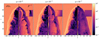 |
Fig. 1. Density (left panels) and inverse of the plasma-β (right panels) for different values of the resistivity, in logarithmic scale at t = 300. The left, middle, and right panel blocks show results computed with resistivity values of η = 10−6, η = 10−3, and η = 10−2, respectively. |
The most prominent differences are related to the electromagnetic field, which is strongly affected by the physical resistivity present in our simulations. We notice (see the zoomed panels of Fig. 1) a much steeper gradient in the magnetization at the interface (contact discontinuity) between the jet plasma and the shocked ambient medium (from two orders of magnitude in the low-η case to a smooth transition in the high-η case). Such a feature is not visible while looking at the density profile and is related to the suppression, due to the smearing of magnetic gradients, of the magnetic field turbulence caused by the interaction between the jet gas and the ambient medium. As a result, the jet magnetization is suppressed for the largest value of η.
For low and moderate values of the resistivity (i.e., η ≲ 10−3), the jets show multiple zones with an average magnetization between 0.1 and 10, which is comparable to previous RRMHD reconnection studies (Del Zanna et al. 2016; Ripperda et al. 2019b), suggesting that large-scale magnetic reconnection and plasmoid formation may occur in such locations (see the next subsection). In the cited works, the plasma magnetization was set as an initial parameter, which is independent of the resistivity; here, despite the same initial physical conditions both at injection and in the ambient plasma for all our simulations, the final jet magnetization is strictly interrelated with the physical resistivity.
The impact of the resistivity reflects on the large-scale evolution of the field, as can be shown by computing the injected electromagnetic energy, defined as (see Perucho et al. 2019)
 (30)
(30)
where f is the jet tracer. This is shown in Fig. 2 as a function of time. The solid lines represent the values of the injected energy normalized to the final value of the run with η = 10−6. In the very early evolutionary phases, the middle and low resistivity cases are almost indistinguishable. However, around t ∼ 35 the two cases start showing some differences, since the jet head has already started interacting with the surrounding medium, slowing down the propagation and triggering the turbulence. Such differences are much more prominent while looking at the high diffusivity cases, in terms of both timescale and the suppression of electromagnetic energy. At time t ∼ 300 the ratio between the injected energy is ∼0.64 between the middle and the low resistivity and ∼0.15 between the high and the low resistivity cases.
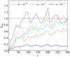 |
Fig. 2. Jet-injected electromagnetic energy. The solid lines represent the energy normalized to the final value of the run with η = 10−6, while the dashed lines represent the same quantities normalized to the final values of each corresponding simulation. |
The dashed lines of Fig. 2 represent the fraction of injected energy normalized with respect to the final value of each simulation (the solid and dashed cyan lines overlap since their normalization is equivalent). We note that the cases with higher resistivity reach a higher fraction of their final injected energy much earlier on. Such differences could also be related to the contribution provided by the resistive field, which becomes less negligible for higher values of η (see a wider discussion in Sect. 3.2.2). This, in addition to the higher field diffusion (as shown by the maps of β−1), may contribute to explaining this behavior.
On the other hand, the impact of the lower jet magnetization and higher resistive electric field for increasing values of η on the jet shape is much less evident (see Fig. 3). This is shown by the low and medium resistivity cases, the jet width of which (defined as the largest r-coordinate of the interface between the jet and the cocoon) differs from each other by ≲10%. On the other hand, the high resistivity case yields a slower (for most of the evolution) and wider jet. The impact of the resistivity on the jet shape becomes more relevant after the turbulence has fully developed within the jet. In particular, differences in the jet width or head (defined as the largest z coordinate of the interface between the jet and the cocoon) are not seen (≲1%) until t ≳ 70.
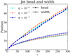 |
Fig. 3. Jet head (circles) and width (crosses) positions for different values of resistivity, computed as functions of time. |
3.2.1. The formation of current sheets
As we have seen, the most prominent differences among the propagating jets at various values of (constant) η are related to the electromagnetic field, which is strongly affected by its diffusion caused by the nonideal processes occurring in our simulations. More specifically, the higher diffusion of the magnetic field leads to a smearing of the poloidal component, resulting in the suppression of the flow and magnetic vortexes typical of MHD turbulence (see the zoomed-in panels of Fig. 4).
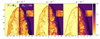 |
Fig. 4. Toroidal component of the magnetic field’s curl (left panel blocks, representing a proxy for the toroidal current) and poloidal magnetic field (right panel blocks) for different values of resistivity, in logarithmic scale at t = 300. The left, middle, and right panel blocks show results computed with resistivity values of η = 10−6, η = 10−3, and η = 10−2, respectively. |
Turbulence in plasmas is known to lead to the formation of current sheets and to reconnection events, and this is particularly important in relativistic magnetically dominated plasmas where the release of energy could be huge. Relativistic magnetic reconnection is also becoming a paradigm for high-energy particle acceleration (e.g., Sironi & Spitkovsky 2014; Sironi et al. 2015; Petropoulou et al. 2019; Medina-Torrejón et al. 2021). The large (temporal and spatial) scale separation between plasma dissipative processes (at the electron/ion skin-depth level) and jet dynamics (up to kpc scales) prevents current numerical models from resolving all the relevant physical phenomena at once (as stated in Medina-Torrejón et al. 2023). Therefore, we focus here on the largest scale scenario dictated by the propagation of astrophysical jets, treated in the fluid/MHD approximation, and we cannot investigate the detailed reconnection scales and (kinetic) physics involved at the same time.
In order to more systematically detect possible reconnection sites, we focus on the structure of the poloidal magnetic field and its curl, that is, the non-relativistic current Jϕ = (∇×B)ϕ, as is often done in the literature, even by devising specific detectors based on this quantity (e.g., Zhdankin et al. 2013; Nurisso et al. 2023). Therefore, in Fig. 4 we show maps of the non-relativistic toroidal current and of the poloidal field from which the former quantity has been computed. As a first consideration, we point out that current sheets and magnetic islands can also appear in simulations without an explicit physical resistivity (ideal MHD), due to the intrinsic and unavoidable diffusivity of the numerical schemes. Properties such as the width of the current sheets arising from the ideal simulations are strictly related to the grid resolution and the numerical schemes. Here we have verified that our ideal runs are very close to the case with η = 10−6, meaning that high-order reconstruction is able to maintain at the minimum level the numerical diffusivity (comparable with the ideal simulations), in spite of the use of the HLL approximate Riemann solver.
Because of the lack of turbulence caused by the physical resistivity in the most dissipative case with η = 10−2, the formation of current sheets is largely reduced compared with the other two cases. In particular, thicker current sheets are formed only in selected regions, for example near the axis and the jet head and between the jet material and the bow shock. Conversely, a lower resistivity leads to more ubiquitous and thinner current sheet regions. The strong dependence of the formation of current sheets on higher magnetization, maintained only in the lower resistivity runs, is promising, given that astrophysical plasmas are expected to be quasi-ideal and favorable for the turbulent reconnection scenario.
In Fig. 5 we have isolated four different regions from the case η = 10−3 where the magnetic field shows an inversion of its polarity and becomes prone to the formation of relativistic current sheets (which are a primary ingredient of magnetic reconnection). Each region shows one or multiple inversions of the magnetic field lines due to the turbulence within the jet, and the consequent tearing instability leading to the plasmoids. Despite the lack of resolution required in order to properly resolve the complex internal structure of the magnetic islands, we were able to select several portions of each region where the magnetic field polarity is suitable for magnetic reconnection and plasmoid instability, allowing us to properly detect the X- and O-points in current sheets (as shown in the zoomed-in panels). All the panels selected (but the top right, number two) show an average magnetization between 0.1 and 10 (see Fig. 1), since a lower magnetization may not lead to the formation of plasmoids (Ripperda et al. 2019b). Moreover, as shown in the right panel of Fig. 5, notice that the electric and magnetic contributions to the electromagnetic density are comparable in the jet region, mostly due to the high speed flows. Higher resolution simulations are expected to resolve the X- and O-points to a better accuracy, showing the regions inside current sheets where the electric field becomes stronger than the magnetic field.
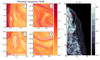 |
Fig. 5. Current sheet forming in the turbulent jet region for the case η = 10−3 at t = 300. The right panel shows the ratio between the electric and magnetic components of the electromagnetic energy. The four left panels show zoomed-in portions of the jet domain (see the rectangles in the right plot), where the poloidal magnetic field (color) and magnetic field lines (white lines) are plotted in order to highlight the reversal of the magnetic field and the formation of magnetic islands due to magnetic reconnection. |
Despite the strong jet magnetization in terms of magnetic energy, comparable to the thermal one (at least in the lower resistivity cases), when the interaction with the ambient medium starts, the resulting relativistic magnetization is strongly suppressed by the mixing, given that the ambient medium is a thousand times denser than the jet. The interface at the contact discontinuity is prone to the Kelvin-Helmholtz instability, due to the strong shear velocities, and this is the main trigger for this mixing. However, the same instability enhances the turbulence level and favors in turn magnetic reconnection, as shown by the presence of the X-points and magnetic islands in the zoomed-in panels also present in these regions.
3.2.2. The resistive electric field
In addition to the formation of current sheets and plasmoids, the resistive component of the electric field is also an indicator of sites where nonideal processes may take place. Since this term can only appear if a physical explicit resistivity coefficient is present, magnetic reconnection in relativistic plasmas should be addressed through consistent numerical recipes, in other words by employing resistive relativistic MHD schemes with explicit resistivity, as is properly achieved here.
The presence of such nonideal components of the electric field can be highlighted by displaying quantities like E ⋅ v and E ⋅ B, since they both vanish in ideal MHD (and relativistic MHD). These are shown in Fig. 6, the parallel electric field component with respect to the velocity in the left panel block and the parallel electric field component with respect to the magnetic field in the right panel block, for the intermediate (left panels) and high (right panels) diffusivity models. We note that those components vanish at the injection region by construction (we recall that an ideal electric field is assumed there, in the radial direction). In the presence of a high resistivity, the resistive electric field starts to arise closer to the jet base (see Fig. 6).
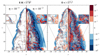 |
Fig. 6. Normalized parallel component of the electric field. For each panel group, E ⋅ B (left panel blocks) and E ⋅ v (right panel blocks) are shown for different values of the diffusivity at t = 300 in a symmetric logarithmic scale. The parallel components are normalized with respect to the corresponding quantities. The left and right panels of each block show results computed with resistivity values of η = 10−3 and η = 10−2, respectively. |
Since the numerical resistivity is dominant in the lowest resistivity model, we do not show here the corresponding resistive electric field. Instead, we focus on the models whose physical diffusivity overcomes the numerical dissipation, since the resistive properties can be derived more consistently.
Because of the very turbulent structure of the magnetic field, the intermediate diffusivity case yields small layers with different polarity (see the zoomed-in panels of Fig. 6). Due to the “poor” resolution, such layers are separated by a very limited number of computational cells. The most evident difference between the medium and high resistivity cases is given by the electric field orientation. As shown by the left and middle panel blocks of Fig. 6, the parallel component in the η = 10−3 case shows, throughout the whole jet, an angle (given by the normalization of the scalar product between the electric field and the magnetic/velocity field) closer to 90° than the high resistivity case.
We also notice that in both resistive regimes the resulting spatial structure of E ⋅ B is quite a bit smoother with respect to E ⋅ v, especially for the η = 10−2 case, where larger scales are clearly produced. As discussed previously, this is not surprising, since the dissipation scale of the magnetic field is determined by the values of the physical resistivity, while the turbulent velocity structure is more affected by the intrinsic diffusion of the numerical algorithms. We note that a stronger relevance of the parallel component does not necessarily mean a stronger resistive electric field, since the electromagnetic energy depends on the diffusivity as well.
In addition to the different relevance of the parallel component, the case with high resistivity shows a smoother transition of the parallel component from the jet to the outer ambient medium (where it is absent by construction). In particular, the parallel electric field, in the presence of higher resistivity, is also diffused outward more rapidly in the region between the turbulent material and the bow shock (especially when looking at the parallel component with respect to the magnetic field).
A final consideration can be done on the impact of the finite conductivity on the jet-dissipated power, the definition of which in the fluid comoving frame is
 (31)
(31)
Nonideal MHD processes (e.g., resistivity) usually involve an energy conversion; in this case, the magnetic energy is converted into thermal energy. As shown in Fig. 7, a higher resistivity leads to a more efficient energy conversion rate and heat generation through all the jet up to the bow shock. On the other hand, the case η = 10−3 shows significant power dissipated near the jet head and, more generally, in the jet regions where magnetic reconnection is more likely to take place. Such behavior is consistent with the fact that the reconnection process involves a conversion from magnetic energy to kinetic, thermal, and particle (on much smaller scales than the one typical of these simulations) energy.
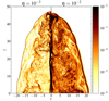 |
Fig. 7. Jet-dissipated power of the η = 10−3 (left panel) and the η = 10−2 (right panel) resistivity models at t = 300 in logarithmic scale. |
3.3. Variable resistivity models
A constant resistivity profile, albeit a very simple and effective strategy, may not consistently model the differences between the jet and the ambient medium. In this section we compare two more consistent, non-constant (in both time and space) resistivity models. The assumption of a resistivity confined in the jet is justified, as in Fendt & Čemeljić (2002), by the turbulent (and thus resistive) nature of the accretion disks. For instance, Qian et al. (2018), Vourellis et al. (2019) assumes a resistivity caused by the thin accretion disk rotation, which triggers the magneto-rotational instability. A similar assumption is made by Bugli et al. (2014), Tomei et al. (2020) in the context of mean-field dynamo in thick accretion tori. Moreover, turbulence is also supposed to be generated in the vicinity of black holes (Nathanail et al. 2022), leading to the formation of plasmoids for up to ∼40 gravitational radii. It is therefore natural to expect that the turbulent/resistive nature of the accretion flow is present also in the outflow at a greater distance from the accreted matter.
A simple yet effective way to model a more consistent diffusivity profile is to relate it to the passive scalar tracer:
 (32)
(32)
Since the passive tracer has values between 0 (ambient) and 1 (jet), the resistivity will always be bound between 10−6 and 10−3. Here the resistivity is mostly determined by the mixing of jet and ambient medium, while the electromagnetic components are only included from the full evolution of the RRMHD equations.
A more consistent resistivity profile is computed, similar to that in Fendt & Čemeljić (2002), by fixing the Lundquist number, S, yielding
 (33)
(33)
where  is the Alfvén speed and L, a typical length scale of the system, is set to be equal to the injection radius, rj = 1. Here, in contrast to Fendt & Čemeljić (2002), we consider the whole magnetic field (i.e., toroidal and poloidal) instead of only the poloidal field. We chose a value of S = 103 in order to reproduce a proper physical resistivity (i.e., higher than the numerical dissipation) in a suitable range to model astrophysical plasmas.
3.3.1. Magnetic field and magnetization
In Fig. 8, we show the toroidal current and the poloidal magnetic field of the constant low resistivity model (here used as a proxy for the numerical dissipation) compared with the two more consistent resistivity profiles (henceforth Tr-case and S-case). As a first consideration, we notice how the turbulent pattern of the poloidal magnetic field features the same level of turbulence (see Appendix B). Another similarity between all these runs is the formation of current sheets, highlighted by the toroidal component of the (classical) current, (∇ × B)ϕ, through the entire jet domain. The jet head and axis, as well as the region between the jet and the bow shock, remain the locations where current sheets are more likely to be located, but the turbulent region (especially in the S-case) is equally promising as a source of nonthermal particles due to magnetic reconnection.
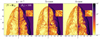 |
Fig. 8. Toroidal current (left panel blocks, computed from the curl of the magnetic field) and poloidal magnetic field (right panel blocks) for different values of the resistivity, in logarithmic scale. The left, middle, and right panel blocks show results computed, respectively, with a constant resistivity of η = 10−6, the Tr-case, and the S-case. |
However, the injected energy (shown in Fig. 9), in both cases with nonuniform resistivity, saturates at lower values (∼75% of the low constant resistivity case). This different saturation is caused by the different values that the resistivity can assume during the temporal evolution. By computing the average value of the jet resistivity as
 (34)
(34)
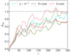 |
Fig. 9. Jet-injected electromagnetic energy of different resistivity models at t = 300 in logarithmic scale. The solid lines represent the energy normalized to the final value of the run with constant (in space and time) resistivity η = 10−6, while the dashed lines represent the same quantities normalized to the final values of each corresponding simulation. |
we notice a different saturation of such a value. More specifically, already at t ∼ 30, the average jet resistivity has reached a value of 2.5 × 10⁻⁴ in the S-case, which remains quite constant throughout the rest of the simulation. On the other hand, the average jet resistivity in the Tr-case starts with a value of ∼10−3 as the jet is injected (t ≳ 0), since the jet and ambient matter have not started to interact yet; then at around t ∼ 100 the jet and the ambient medium have already interacted and the average jet resistivity slowly converges to 4.5 × 10⁻⁴ until the end of the simulation.
This confirms the trend seen in Fig. 2, where a higher resistivity leads to a weaker injected energy. Moreover, it explains why the case S = 103 reaches the saturation of the injected energy earlier on; since the resistivity decreases because of the mixing, the saturation value increases as the turbulence develops.
We also notice that the spatial resistivity profile shows clear differences between the different resistivity models. More specifically, the Tr-case shows a resistivity dominated by the jet at earlier time (see the left panel of Fig. 10), and even at later times a difference of almost two orders of magnitude are present between the resistivity at the lower regions and the jet head. On the other hand, the S-case shows a more uniform diffusivity distribution, since a stronger magnetic field triggers a higher resistivity that diffuses the magnetic field. This “cycle” of magnetic field and diffusivity has already converged at t ≲ 50, as shown in the left panels of Fig. 10.
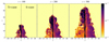 |
Fig. 10. Resistivity computed at different times (t = 100, 200, 300, respectively, in the left, middle, and right panel blocks) with the two different variable resistivity models (Tr-case in the left panels and S-case in the right panels, respectively). |
3.3.2. The resistive electric field
As for the constant diffusivity models, the nonideal electric field is a key component in order to investigate the role of the resistive features. In particular, in Fig. 11 we show the parallel component of the electric field with respect to the magnetic field.
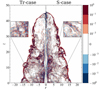 |
Fig. 11. Parallel (normalized, as in Fig. 6) component of the electric field respect to the magnetic field for the Tr-case (left panel) and the S-case (right panel) resistivity models at t = 300 in symmetric logarithmic scale. |
In both cases, the polarity of the parallel electric field near the boundary between jet and environment is the opposite with respect to the cases shown in Sect. 3.2.2 (i.e., η = 10−3 and η = 10−2). This feature is not surprising, since while investigating constant diffusivity models (see Sect. 3.2.2) we noticed such inversion in the presence of a numerical resistivity (which is the case at the interface between the jet and the ambient medium for both variable diffusivity models).
However, the parallel electric field arises near the jet base because of the higher physical resistivity at the jet base. The development of a strong parallel component in this region was also seen in the η = 10−3 and η = 10−2 cases. As a result, the jet location where the parallel field becomes more relevant is near the axes, in agreement with the η = 10−3 case.
The spatial structure of E ⋅ B is significant less smooth than the cases with constant resistivity because of the lower values of resistivity outside the very inner propagation region. Moreover, the two models show a consistent difference in terms of the spatial distribution of the parallel field. In particular, both cases show a relevant parallel component in the turbulent region, which is suppressed in the η = 10−3 case.
The sharp gradient of the parallel field at the interface between the jet and the ambient medium is likely due to the numerical diffusivity, as in both models the value of η drops abruptly in the jet’s environment. For the same reason, there is also a lack of diffused parallel field beyond that interface, as opposed to the models with constant resistivity (see the first panel of Fig. 6).
4. Discussion and conclusions
In this paper we present the first systematic numerical study, in the regime of RRMHD, of astrophysical relativistic jets endowed with both poloidal and toroidal magnetic field components propagating through a uniform magnetized medium. We combined a high resolution grid in cylindrical coordinates with high-order numerical algorithms and realistic physical assumptions in order to achieve the best level of refinement, while preserving the robustness required to overcome the numerical issues that often arise when simulating relativistic flows in a strongly magnetized regime.
The following summarizes our approaches and results:
-
We extended the IMEX scheme to the use of the Taub EoS in order to couple an accurate and robust evolution scheme for the electric field in nonideal conditions and the proper treatment of the gas-varying conditions from the jet to the ambient medium. We also augmented the stability of the IMEX scheme by improving the choice of the initial primitive variables used during the implicit step.
-
We investigate the role of a constant (in space and time) resistivity coefficient. More specifically, we find that a high resistivity coefficient, say η ∼ 10−2 in typical code units, corresponding to a Lundquist number of roughly S ∼ 100 (normalized to the injection length and for an Alfvén speed close to the speed of light), almost completely suppresses the turbulence in the propagating jet and therefore the formation of relativistic current sheets. Conversely, a lower resistivity (at least η ≲ 10−3, or S ≳ 103) triggers the formation of multiple zones that could be prone (in terms of magnetization and field topology) to the plasmoid instability.
-
The electric field, in the presence of a physical resistivity, develops a component parallel to the magnetic field that can be used as an indicator of nonideal processes occurring at the turbuent scale, even in the absence of magnetic reconnection events. We found that different values of resistivity strongly impact the emergence of the resistive/parallel electric field, leading to a different spatial structure and dissipated power.
-
The combination of high-order numerical algorithms and high resolution enables us to find with increased accuracy the formation of X- and O-points within the jets, despite the lack of resolution required to resolve the particle acceleration scales. However, selected zones of the large-scale jets can provide more consistent recipes in order to investigate the reconnection process at smaller scales.
-
We also adopted and compared more consistent diffusivity models with a variable coefficient, η, one based on a passively evolved scalar jet tracer, and another one fixing a constant value for the Lundquist number. Such models feature a more refined level of turbulence with respect to the case of intermediate constant diffusivity, consistent with the fact that the resistivity in the jet varies in the range 10−5 < η < 10−3. However, the injected energy saturates at different levels and at different times, because of the spatial and temporal variations in the resistivity. In our opinion, the recipe based on a constant Lundquist number, that is, η = vAL/S (L is a typical scale, here the injection width, and vA is the Alfvén speed), is to be preferred for both computational reasons (it is not subject to the numerical diffusion of an advected passive scalar) and physical ones (the resistivity is basically proportional to the local magnetization), so we recommend its use.
In conclusion, let us briefly discuss some important physical implications and possible lines of future development of the present work.
As illustrated by our simulations, the importance of addressing the large difference in scale between jet and fundamental plasma dynamics cannot be overstated. The use of high-accuracy numerical schemes is thus crucial to quantitatively assess the impact of turbulent diffusion in relativistic jets. Future work will therefore need to improve upon this aspect, for example by considering global high-order schemes (Berta et al. 2023).
Another debated issue is the possible role played by the resistive electric field, that is the nonideal component proportional to the current density in the simplest Ohmic-type modelization, especially for the acceleration of the highest energy particles (see, e.g., Kowal et al. 2009; Medina-Torrejón et al. 2021; Sironi 2022; Puzzoni et al. 2022 and references therein). A possible scenario arising from PIC simulations is that the nonideal field (at X-points) plays an important role in nonthermal particle acceleration in microscopic current sheets as it starts the acceleration process. After this, the Fermi-type acceleration via the ideal electric field in the evolving plasmoids takes over and most of the particle energy is gained (e.g., Guo et al. 2019). At the much larger macroscopic scale of astrophysical jets, further acceleration is likely to take place via the ideal electric field of MHD turbulence (e.g., Medina-Torrejón et al. 2023). This large-scale Fermi acceleration can be studied using test particles or PIC-MHD methods (Mignone et al. 2018a; Vaidya et al. 2018; Medina-Torrejón et al. 2023), even in the context of propagating relativistic jets.
Due to the large difference between them, the precise interplay between goings-on at microscopic scales (i.e., the current sheets typically studied via PIC simulations) and the vast scales typical of MHD simulations of astrophysical sources is still very unclear. However, we would like to stress here that since the real resistivity is orders of magnitude lower than the values adopted in this paper (and the numerical diffusivity typical of any ideal relativistic MHD simulation), the latter should not be strictly interpreted as the microscopic resistivity coming from the PIC simulations, but rather as an effective “sub-grid” resistivity attempting to model the impact of unresolved and nonideal kinetic processes on larger scales. The effectiveness of such sub-grid models (which in several cases combine turbulent diffusion and mean-field dynamo action) has been positively tested in different astrophysical contexts by means of high-resolution studies (e.g., Liska et al. 2020; Tomei et al. 2020; Guilet et al. 2022; Reboul-Salze et al. 2022; Kiuchi et al. 2023). More refined resistivity models (see, e.g., Selvi et al. 2023) will be able to mimic with even better consistency the impact of microscopic kinetic process on the large-scale scenario.
Other than AGN and blazar jets, the type of resistive simulations described here could also apply to different type of sources. A noticeable example is provided by the short-GRB jets arising from BNS merger multimessenger events (Pavan et al. 2021, 2023), where the magnetic field is known to play a crucial role (Ciolfi 2020). For relativistic jets propagating in such a complex and structured magnetized environment, a finite conductivity is expected to be important and to lead to very different observational signatures, so this will certainly be a direction for future investigation.
Unfortunately, in Del Zanna & Bucciantini (2018), Mignone et al. (2019) the last term with the Levi-Civita tensors was forgotten, while all the other equations in those works are correct.
Acknowledgments
We thank Christian Fendt for useful comments/discussions. L.D.Z., A.P., R.C., and A.M. acknowledge support from the PRIN-INAF 2019 Grant “Short gamma-ray burst jets from binary neutron star mergers” (Ob. fu. 1.05.01.85.16). All the simulations were performed on GALILEO100 and MARCONI100 clusters at CINECA (Bologna, Italy). In particular, we acknowledge CINECA for the availability of high performance computing resources and support through an award under the MoU INAF-CINECA (Grant INA23_C9B05) and through a CINECA-INFN agreement, providing the allocations INF22_teongrav and INF23_teongrav. This project has received funding from the European Union’s Horizon Europe research and innovation programme under the Marie Skłodowska-Curie grant agreement No 101064953 (GR-PLUTO), and by ICSC – Centro Nazionale di Ricerca in High Performance Computing, Big Data and Quantum Computing, funded by European Union – NextGenerationEU.
References
- Abbott, B. P., Abbott, R., Abbott, T. D., et al. 2017, ApJ, 848, L12 [Google Scholar]
- Anile, A. M. 2005, Relativistic Fluids and Magneto-fluids (Cambridge: Cambridge University Press) [Google Scholar]
- Balsara, D. 2001, ApJS, 132, 83 [NASA ADS] [CrossRef] [Google Scholar]
- Beckwith, K., & Stone, J. M. 2011, ApJS, 193, 6 [NASA ADS] [CrossRef] [Google Scholar]
- Begelman, M. C., Blandford, R. D., & Rees, M. J. 1984, Rev. Mod. Phys., 56, 255 [Google Scholar]
- Berta, V., Mignone, A., Bugli, M., & Mattia, G. 2023, J. Comput. Phys., submitted [arXiv:2310.11831] [Google Scholar]
- Blandford, R., Meier, D., & Readhead, A. 2019, ARA&A, 57, 467 [NASA ADS] [CrossRef] [Google Scholar]
- Bodo, G., Tavecchio, F., & Sironi, L. 2021, MNRAS, 501, 2836 [NASA ADS] [CrossRef] [Google Scholar]
- Bucciantini, N., & Del Zanna, L. 2013, MNRAS, 428, 71 [NASA ADS] [CrossRef] [Google Scholar]
- Bugli, M., Del Zanna, L., & Bucciantini, N. 2014, MNRAS, 440, L41 [CrossRef] [Google Scholar]
- Cerutti, B., Werner, G. R., Uzdensky, D. A., & Begelman, M. C. 2014, ApJ, 782, 104 [CrossRef] [Google Scholar]
- Chernoglazov, A., Ripperda, B., & Philippov, A. 2021, ApJ, 923, L13 [NASA ADS] [CrossRef] [Google Scholar]
- Ciolfi, R. 2020, Gen. Relat. Gravit., 52, 59 [CrossRef] [Google Scholar]
- Comisso, L., & Sironi, L. 2018, Phys. Rev. Lett., 121, 255101 [NASA ADS] [CrossRef] [Google Scholar]
- Dedner, A., Kemm, F., Kröner, D., et al. 2002, J. Comput. Phys., 175, 645 [Google Scholar]
- Del Zanna, L., & Bucciantini, N. 2018, MNRAS, 479, 657 [NASA ADS] [Google Scholar]
- Del Zanna, L., Bucciantini, N., & Londrillo, P. 2003, A&A, 400, 397 [NASA ADS] [CrossRef] [EDP Sciences] [Google Scholar]
- Del Zanna, L., Zanotti, O., Bucciantini, N., & Londrillo, P. 2007, A&A, 473, 11 [NASA ADS] [CrossRef] [EDP Sciences] [Google Scholar]
- Del Zanna, L., Papini, E., Landi, S., Bugli, M., & Bucciantini, N. 2016, MNRAS, 460, 3753 [Google Scholar]
- Del Zanna, L., Tomei, N., Franceschetti, K., Bugli, M., & Bucciantini, N. 2022, Fluids, 7, 87 [NASA ADS] [CrossRef] [Google Scholar]
- Event Horizon Telescope Collaboration 2019, ApJ, 875, L1 [Google Scholar]
- Felker, K. G., & Stone, J. M. 2018, J. Comput. Phys., 375, 1365 [NASA ADS] [CrossRef] [Google Scholar]
- Fendt, C., & Čemeljić, M. 2002, A&A, 395, 1045 [NASA ADS] [CrossRef] [EDP Sciences] [Google Scholar]
- Gottlieb, S., Shu, C.-W., & Tadmor, E. 2001, SIAM Rev., 43, 89 [NASA ADS] [CrossRef] [Google Scholar]
- Guilet, J., Reboul-Salze, A., Raynaud, R., Bugli, M., & Gallet, B. 2022, MNRAS, 516, 4346 [NASA ADS] [CrossRef] [Google Scholar]
- Guo, F., Li, X., Daughton, W., et al. 2019, ApJ, 879, L23 [Google Scholar]
- Harten, A., Lax, P., & Leer, B. 1983, SIAM Rev., 25, 35 [CrossRef] [Google Scholar]
- Kiuchi, K., Reboul-Salze, A., Shibata, M., & Sekiguchi, Y. 2023, ArXiv e-prints [arXiv:2306.15721] [Google Scholar]
- Komissarov, S. S. 2007, MNRAS, 382, 995 [CrossRef] [Google Scholar]
- Komissarov, S. S., Barkov, M., & Lyutikov, M. 2007, MNRAS, 374, 415 [Google Scholar]
- Kowal, G., Lazarian, A., Vishniac, E. T., & Otmianowska-Mazur, K. 2009, ApJ, 700, 63 [Google Scholar]
- Lee, C.-F., Hwang, H.-C., Ching, T.-C., et al. 2018, Nat. Comm., 9, 4636 [NASA ADS] [CrossRef] [Google Scholar]
- Leismann, T., Antón, L., Aloy, M. A., et al. 2005, A&A, 436, 503 [NASA ADS] [CrossRef] [EDP Sciences] [Google Scholar]
- Liska, M., Tchekhovskoy, A., & Quataert, E. 2020, MMRAS, 494, 3656 [CrossRef] [Google Scholar]
- Londrillo, P., & Del Zanna, L. 2004, J. Comput. Phys., 195, 17 [NASA ADS] [CrossRef] [Google Scholar]
- Loureiro, N. F., & Uzdensky, D. A. 2016, Plasma Phys. Control. Fusion, 58, 014021 [CrossRef] [Google Scholar]
- Lyubarsky, Y. E. 2005, MNRAS, 358, 113 [NASA ADS] [CrossRef] [Google Scholar]
- Lyutikov, M., & Uzdensky, D. 2003, ApJ, 589, 893 [NASA ADS] [CrossRef] [Google Scholar]
- Medina-Torrejón, T. E., de Gouveia Dal Pino, E. M., Kadowaki, L. H. S., et al. 2021, ApJ, 908, 193 [CrossRef] [Google Scholar]
- Medina-Torrejón, T. E., de Gouveia Dal Pino, E. M., & Kowal, G. 2023, ApJ, 952, 168 [CrossRef] [Google Scholar]
- Mignone, A. 2014, J. Comput. Phys., 270, 784 [Google Scholar]
- Mignone, A., & Bodo, G. 2006, MNRAS, 368, 1040 [Google Scholar]
- Mignone, A., & McKinney, J. C. 2007, MNRAS, 378, 1118 [Google Scholar]
- Mignone, A., & Tzeferacos, P. 2010, J. Comput. Phys., 229, 2117 [Google Scholar]
- Mignone, A., Plewa, T., & Bodo, G. 2005, ApJS, 160, 199 [CrossRef] [Google Scholar]
- Mignone, A., Bodo, G., Massaglia, S., et al. 2007, ApJS, 170, 228 [Google Scholar]
- Mignone, A., Ugliano, M., & Bodo, G. 2009, MNRAS, 393, 1141 [NASA ADS] [CrossRef] [Google Scholar]
- Mignone, A., Zanni, C., Tzeferacos, P., et al. 2012, ApJS, 198, 7 [Google Scholar]
- Mignone, A., Bodo, G., Vaidya, B., & Mattia, G. 2018a, ApJ, 859, 13 [CrossRef] [Google Scholar]
- Mignone, A., Mattia, G., & Bodo, G. 2018b, Phys. Plasmas, 25, 092114 [NASA ADS] [CrossRef] [Google Scholar]
- Mignone, A., Mattia, G., Bodo, G., & Del Zanna, L. 2019, MNRAS, 486, 4252 [NASA ADS] [CrossRef] [Google Scholar]
- Miranda-Aranguren, S., Aloy, M. A., & Rembiasz, T. 2018, MNRAS, 476, 3837 [Google Scholar]
- Mizuno, Y. 2013, ApJS, 205, 7 [NASA ADS] [CrossRef] [Google Scholar]
- Nathanail, A., Mpisketzis, V., Porth, O., Fromm, C. M., & Rezzolla, L. 2022, MNRAS, 513, 4267 [NASA ADS] [CrossRef] [Google Scholar]
- Núñez-de la Rosa, J., & Munz, C.-D. 2016, MNRAS, 460, 535 [CrossRef] [Google Scholar]
- Nurisso, M., Celotti, A., Mignone, A., & Bodo, G. 2023, MNRAS, 522, 5517 [NASA ADS] [CrossRef] [Google Scholar]
- Palenzuela, C., Lehner, L., Reula, O., & Rezzolla, L. 2009, MNRAS, 394, 1727 [Google Scholar]
- Pareschi, L., & Russo, G. 2005, J. Sci. Comput., 25, 129 [MathSciNet] [Google Scholar]
- Pavan, A., Ciolfi, R., Kalinani, J. V., & Mignone, A. 2021, MNRAS, 506, 3483 [CrossRef] [Google Scholar]
- Pavan, A., Ciolfi, R., Kalinani, J. V., & Mignone, A. 2023, MNRAS, 524, 260 [NASA ADS] [CrossRef] [Google Scholar]
- Perucho, M., Martí, J.-M., & Quilis, V. 2019, MNRAS, 482, 3718 [NASA ADS] [CrossRef] [Google Scholar]
- Petropoulou, M., Sironi, L., Spitkovsky, A., & Giannios, D. 2019, ApJ, 880, 37 [Google Scholar]
- Puzzoni, E., Mignone, A., & Bodo, G. 2021, MNRAS, 508, 2771 [CrossRef] [Google Scholar]
- Puzzoni, E., Mignone, A., & Bodo, G. 2022, MNRAS, 517, 1452 [NASA ADS] [CrossRef] [Google Scholar]
- Qian, Q., Fendt, C., Noble, S., & Bugli, M. 2017, ApJ, 834, 29 [Google Scholar]
- Qian, Q., Fendt, C., & Vourellis, C. 2018, ApJ, 859, 28 [NASA ADS] [CrossRef] [Google Scholar]
- Reboul-Salze, A., Guilet, J., Raynaud, R., & Bugli, M. 2022, A&A, 667, A94 [NASA ADS] [CrossRef] [EDP Sciences] [Google Scholar]
- Rezzolla, L., & Zanotti, O. 2013, Relativistic Hydrodynamics (Oxford: Oxford University Press) [CrossRef] [Google Scholar]
- Ripperda, B., Bacchini, F., Porth, O., et al. 2019a, ApJS, 244, 10 [NASA ADS] [CrossRef] [Google Scholar]
- Ripperda, B., Porth, O., Sironi, L., & Keppens, R. 2019b, MNRAS, 485, 299 [CrossRef] [Google Scholar]
- Ripperda, B., Bacchini, F., & Philippov, A. A. 2020, ApJ, 900, 100 [NASA ADS] [CrossRef] [Google Scholar]
- Ripperda, B., Liska, M., Chatterjee, K., et al. 2022, ApJ, 924, L32 [NASA ADS] [CrossRef] [Google Scholar]
- Selvi, S., Porth, O., Ripperda, B., et al. 2023, ApJ, 950, 169 [NASA ADS] [CrossRef] [Google Scholar]
- Sironi, L. 2022, Phys. Rev. Lett., 128, 145102 [CrossRef] [Google Scholar]
- Sironi, L., & Spitkovsky, A. 2014, ApJ, 783, L21 [NASA ADS] [CrossRef] [Google Scholar]
- Sironi, L., Petropoulou, M., & Giannios, D. 2015, MNRAS, 450, 183 [Google Scholar]
- Synge, J. 1957, The Relativistic Gas (New York: North-Holland Publishing Company) [Google Scholar]
- Takamoto, M., & Inoue, T. 2011, ApJ, 735, 113 [CrossRef] [Google Scholar]
- Taub, A. H. 1948, Phys. Rev., 74, 328 [NASA ADS] [CrossRef] [Google Scholar]
- Tomei, N., Del Zanna, L., Bugli, M., & Bucciantini, N. 2020, MNRAS, 491, 2346 [Google Scholar]
- Tomei, N., Del Zanna, L., Bugli, M., & Bucciantini, N. 2021, Universe, 7, 259 [NASA ADS] [CrossRef] [Google Scholar]
- Vaidya, B., Mignone, A., Bodo, G., Rossi, P., & Massaglia, S. 2018, ApJ, 865, 144 [Google Scholar]
- Vourellis, C., Fendt, C., Qian, Q., & Noble, S. C. 2019, ApJ, 882, 2 [NASA ADS] [CrossRef] [Google Scholar]
- Weisskopf, M. C., Hester, J. J., Tennant, A. F., et al. 2000, ApJ, 536, L81 [NASA ADS] [CrossRef] [Google Scholar]
- Woosley, S. E. 1993, ApJ, 405, 273 [Google Scholar]
- Zhang, H., Sironi, L., & Giannios, D. 2021, ApJ, 922, 261 [NASA ADS] [CrossRef] [Google Scholar]
- Zhdankin, V., Uzdensky, D. A., Perez, J. C., & Boldyrev, S. 2013, ApJ, 771, 124 [NASA ADS] [CrossRef] [Google Scholar]
Appendix A: Numerical benchmarks
The implementation in the PLUTO code of the IMEX scheme coupled with the Taub EoS (see Section 2.4) has been tested through a series of test problems, which we report here. In particular, we show two 1D shock tubes (for which the impact of the EoS has been described in Mignone & McKinney 2007) and numerical benchmarks for a 2D Kelvin Helmholtz instability, employing Cartesian coordinates. Since, to the extent of our knowledge, the exact solution of the Riemann problem of the RRMHD equations has not been recovered yet, for the shock tube tests we focused on the regimes where the solution approaches the ideal one (η → 0) and where the solution approaches the frozen limit (η → ∞). In the frozen limit, the hydrodynamic quantities are decoupled from the electromagnetic ones (Mignone et al. 2018b), and therefore the choice of EoS should not affect the solution for the electric and magnetic fields, while the fluid variables obviously evolve differently. Unless stated otherwise, we adopted the same numerical algorithms used for the main simulations.
A.1. Shock tube no. 1 (ST1)
The first shock tube problem (ST1), performed previously by Balsara (2001), Del Zanna et al. (2003), represents a 1D explosion driven by an initial pressure difference (a factor 30 in thermal pressure and 100 in magnetic pressure). We choose a domain of x ∈ [ − 0.5, 0.5] (therefore the discontinuity is placed at x = 0) and a resolution of Nx = 400 grid cells. The initial conditions for the discontinuous quantities are:
 (A.1)
(A.1)
while we set ρ = 1.0, Bx = 5.0, and v = E = 0 throughout the entire domain. We performed two runs with constant uniform resistivity with, respectively, η = 10−6 (to reproduce the ideal limit) and η = 1040 (to reproduce the frozen limit). The final time of each simulation is t = 0.4. As pointed out by Balsara (2001), the emerging wave pattern (in the ideal regime) consists of a contact discontinuity separating two (fast and slow) left-going rarefaction waves from two (fast and slow) right-going shocks. In the frozen limit the solution consists of a similar wave pattern; however, the fast and slow waves are replaced by, respectively, light and sound waves. No rotational discontinuity is seen.
The shock tube results are compared with two reference runs: one computed by solving the ideal relativistic MHD equations with the Taub EoS and one computed by solving the RRMHD equations in the frozen limit with the ideal EoS (Γ = 5/3). Both reference runs were performed by employing the same numerical algorithms stated before (since the ideal relativistic MHD equations do not have a stiff component, the time integration was computed through a 3rd RK time integrator) and a resolution of Nx = 12800.
In Fig. A.1 we show density and the Lorentz factor in the left (top and bottom, respectively) panels, while the squares of the magnetic and electric fields are shown in the right (top and bottom, respectively) panels. For the sake of readability, the solid lines (which represent the reference simulations, the ideal regime in red and the frozen limit with ideal EoS in blue, respectively) are superimposed by a fraction of the data points (1/4, i.e., 100 data points are shown) computed through our novel scheme (triangles for the ideal regime and circles for the frozen limit, respectively). As expected, no impact of the EoS is found on E2 and B2 in the frozen limits, as well as both the electromagnetic field and the fluid variables in the ideal limit. We note that, in the frozen limit, the sound and light waves are split between the fluid and the electromagnetic variables. As a result, in the frozen limit the wave pattern is always composed of two waves for each variable (plus the contact wave for the density).
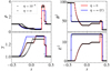 |
Fig. A.1. ST1: comparison of fluid and electromagnetic quantities. On the left panels are shown the fluid density (top) and the Lorentz factor (bottom), while on the right panel the squared norms of the magnetic (top) and electric (bottom) fields are shown. The solid lines represent the reference simulation in the ideal (red) and frozen (blue) limits, respectively, while the test simulations are shown through triangles (ideal limit) and circles (frozen limit). |
A.2. Shock tube no. 2 (ST2)
The second shock tube problem (ST2), again performed by Balsara (2001), Del Zanna et al. (2003), consists of a stronger 1D blast wave (here the jump in thermal pressure is of a factor as high as 104), which yields a more relativistic configuration. The setup is very similar to the previous benchmark; in fact, the only change is in the initial conditions, where discontinuous quantities are initialized as:
 (A.2)
(A.2)
while we set ρ = 1.0, Bx = 10.0, and v = E = 0. The results are shown in the same fashion as the previous benchmark. The solution is composed of two left (fast and slow) rarefaction waves and two right (fast and slow) shocks in the ideal regime, and of two light and sound (left and right) waves in the frozen limit. Again, no rotational discontinuity is shown.
Both the frozen and the ideal limits are reproduced with a great degree of accuracy, as shown in Fig. A.2. The sharp discontinuities located at x ≈ 0.4 are captured in both regimes despite the lower resolution. As pointed out in Mignone & McKinney (2007), the sound speed is highly overestimated while applying an ideal EoS. Such behavior can clearly be seen in the frozen limits, where the density and the Lorentz factor feature discontinuities propagating at the sound speed (as shown by the circles and the solid blue line).
A.3. Kelvin-Helmholtz instability (KHI)
In order to compare the different equations of state and to validate the numerical algorithms adopted in the paper, we performed the Kelvin-Helmholtz instability test of Mizuno (2013). The domain consists of a Cartesian box with x ∈ [ − 0.5, 0.5] and y ∈ [ − 1.0, 1.0], and is filled with an initial constant gas pressure, p = 1.0. The shear velocity profile is given by
 (A.3)
(A.3)
where vsh = 0.5 and a = 0.01 are, respectively, the maximum shear velocity and the characteristic thickness of the double shear layer. The initial density is set to
 (A.4)
(A.4)
where ρh = 1 and ρl = 10−2. The magnetic field is provided in terms of the plasma-β:
 (A.5)
(A.5)
The equilibrium is perturbed by adding
 (A.6)
(A.6)
where the perturbation is characterized by the amplitude A0 = 0.1 and the characteristic length scale of decay α = 0.1. Lastly, we set vz = 0 and we computed the electric field from its ideal condition. The final time of the simulation is t = 15.
In Fig. A.3 we show the growth rate, defined as the volume average of  (top panels) and the growth of the volume-averaged poloidal field (bottom panels) using the ideal (left panels) and the Taub (right panels) EoSs, and the UCT (solid lines) and GLM (x-symbols) algorithms to preserve the non-evolutionary Maxwell equations.
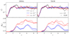 |
Fig. A.3. Kelvin Helmholtz instability. On the left/right panels are plotted the growth rate (top) and the poloidal magnetic field (bottom), shown with ideal/Taub EoS. |
We find good agreement with the values obtained by Mizuno (2013), Mignone et al. (2019); as expected, the growth rate does not show any dependence on the resistivity, regardless of the EoS. Conversely, a higher resistivity is able to quench the poloidal magnetic field amplification, since the latter is caused by the stretching due to the main vortex formation. Moreover, the ideal EoS leads to a stronger amplification of the poloidal magnetic field, in agreement with Mizuno (2013). We also notice very good agreement between the UCT and the GLM algorithms until t = 3, in other words after the nonlinear regime has already taken place.
Appendix B: Turbulence level and resolution
In order to quantify the agreement in the level of turbulence among different models in the paper, we computed the effective resolution of our simulations by computing the normalized gradient ⟨|∇Q|/Q⟩ of the density ρ and the magnetic energy B2/2, similarly to Mignone et al. (2009), Beckwith & Stone (2011).
In Fig. B.1 we show a comparison between all the runs performed in the paper and a reference simulation computed in the ideal relativistic MHD regime and using the same numerical setup presented in Mignone et al. (2009) (but with a resolution matching the one used for our models). All the quantities are normalized to the ones at the final time of the ideal simulation. As expected, all the runs show excellent agreement (i.e., discrepancies are ≲15%) in density (left panel) regardless of the specific value of η, while the magnetic field turbulence is affected by a sufficiently strong physical resistivity. In particular, we notice that the low-resistivity case and the non-constant diffusivity runs show a turbulence that is comparable with the ideal simulation, while the runs with higher resistivity show a lower level of turbulence (65% and 40%, respectively, for the cases η = 10−3 and η = 10−2).
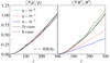 |
Fig. B.1. Effective turbulence resolution (computed as ⟨|∇Q|/Q⟩) of density (left panel) and magnetic energy (right panel) computed for different resistivity models and the ideal simulation using the same setup as Mignone et al. (2009). |
On the other hand, the turbulent scale required a sufficiently high resolution in order to be properly resolved. A "poor" resolution would lead to a higher numerical diffusivity that would strongly affect the turbulent scale and therefore the dynamical evolution of the jet. In order to prove that our resolution is enough to capture the magnetic dissipation scales dictated by the physical resistivity, we compared the normalized gradients for the cases η = 10−3 and η = 10−2 by adopting different grid resolutions. As shown in Fig. B.2, the magnetic turbulence (right panel) shows very good agreement even at half of the reference resolution (i.e., 24 cells per rj), while the poorest resolution model (i.e., 12 cells per rj) shows significant qualitative differences. Concerning the density turbulence, despite slight differences between 36 and 48 cells per rj (≲10%), we find that our reference resolution is high enough to reach convergence. Lower grid resolutions, on the other hand, lead to a more suppressed fluid turbulence.
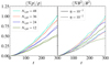 |
Fig. B.2. Same as Fig. B.1, but for different resolution and constant resistivity η = 10−3 (solid line) and η = 10−2 (dashed line). |
All Figures
|
Fig. 1. Density (left panels) and inverse of the plasma-β (right panels) for different values of the resistivity, in logarithmic scale at t = 300. The left, middle, and right panel blocks show results computed with resistivity values of η = 10−6, η = 10−3, and η = 10−2, respectively. |
| In the text | |
|
Fig. 2. Jet-injected electromagnetic energy. The solid lines represent the energy normalized to the final value of the run with η = 10−6, while the dashed lines represent the same quantities normalized to the final values of each corresponding simulation. |
| In the text | |
|
Fig. 3. Jet head (circles) and width (crosses) positions for different values of resistivity, computed as functions of time. |
| In the text | |
|
Fig. 4. Toroidal component of the magnetic field’s curl (left panel blocks, representing a proxy for the toroidal current) and poloidal magnetic field (right panel blocks) for different values of resistivity, in logarithmic scale at t = 300. The left, middle, and right panel blocks show results computed with resistivity values of η = 10−6, η = 10−3, and η = 10−2, respectively. |
| In the text | |
|
Fig. 5. Current sheet forming in the turbulent jet region for the case η = 10−3 at t = 300. The right panel shows the ratio between the electric and magnetic components of the electromagnetic energy. The four left panels show zoomed-in portions of the jet domain (see the rectangles in the right plot), where the poloidal magnetic field (color) and magnetic field lines (white lines) are plotted in order to highlight the reversal of the magnetic field and the formation of magnetic islands due to magnetic reconnection. |
| In the text | |
|
Fig. 6. Normalized parallel component of the electric field. For each panel group, E ⋅ B (left panel blocks) and E ⋅ v (right panel blocks) are shown for different values of the diffusivity at t = 300 in a symmetric logarithmic scale. The parallel components are normalized with respect to the corresponding quantities. The left and right panels of each block show results computed with resistivity values of η = 10−3 and η = 10−2, respectively. |
| In the text | |
|
Fig. 7. Jet-dissipated power of the η = 10−3 (left panel) and the η = 10−2 (right panel) resistivity models at t = 300 in logarithmic scale. |
| In the text | |
|
Fig. 8. Toroidal current (left panel blocks, computed from the curl of the magnetic field) and poloidal magnetic field (right panel blocks) for different values of the resistivity, in logarithmic scale. The left, middle, and right panel blocks show results computed, respectively, with a constant resistivity of η = 10−6, the Tr-case, and the S-case. |
| In the text | |
|
Fig. 9. Jet-injected electromagnetic energy of different resistivity models at t = 300 in logarithmic scale. The solid lines represent the energy normalized to the final value of the run with constant (in space and time) resistivity η = 10−6, while the dashed lines represent the same quantities normalized to the final values of each corresponding simulation. |
| In the text | |
|
Fig. 10. Resistivity computed at different times (t = 100, 200, 300, respectively, in the left, middle, and right panel blocks) with the two different variable resistivity models (Tr-case in the left panels and S-case in the right panels, respectively). |
| In the text | |
|
Fig. 11. Parallel (normalized, as in Fig. 6) component of the electric field respect to the magnetic field for the Tr-case (left panel) and the S-case (right panel) resistivity models at t = 300 in symmetric logarithmic scale. |
| In the text | |
|
Fig. A.1. ST1: comparison of fluid and electromagnetic quantities. On the left panels are shown the fluid density (top) and the Lorentz factor (bottom), while on the right panel the squared norms of the magnetic (top) and electric (bottom) fields are shown. The solid lines represent the reference simulation in the ideal (red) and frozen (blue) limits, respectively, while the test simulations are shown through triangles (ideal limit) and circles (frozen limit). |
| In the text | |
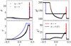 |
Fig. A.2. Same quantities as in Fig. A.1, but here for the ST2 test. |
| In the text | |
|
Fig. A.3. Kelvin Helmholtz instability. On the left/right panels are plotted the growth rate (top) and the poloidal magnetic field (bottom), shown with ideal/Taub EoS. |
| In the text | |
|
Fig. B.1. Effective turbulence resolution (computed as ⟨|∇Q|/Q⟩) of density (left panel) and magnetic energy (right panel) computed for different resistivity models and the ideal simulation using the same setup as Mignone et al. (2009). |
| In the text | |
|
Fig. B.2. Same as Fig. B.1, but for different resolution and constant resistivity η = 10−3 (solid line) and η = 10−2 (dashed line). |
| In the text | |
Current usage metrics show cumulative count of Article Views (full-text article views including HTML views, PDF and ePub downloads, according to the available data) and Abstracts Views on Vision4Press platform.
Data correspond to usage on the plateform after 2015. The current usage metrics is available 48-96 hours after online publication and is updated daily on week days.
Initial download of the metrics may take a while.