| Issue |
A&A
Volume 693, January 2025
|
|
|---|---|---|
| Article Number | A4 | |
| Number of page(s) | 18 | |
| Section | Planets, planetary systems, and small bodies | |
| DOI | https://doi.org/10.1051/0004-6361/202452127 | |
| Published online | 23 December 2024 | |
Homogeneous planet masses
I. Reanalysis of archival HARPS radial velocities
1
European Southern Observatory,
Karl-Schwarzschild-Str. 2,
85748
Garching bei München,
Germany
2
Mullard Space Science Laboratory, University College London,
Dorking
RH5 6NT,
UK
3
University Observatory Munich, Ludwig-Maximilians-Universität,
Scheinerstr. 1,
81679
Munich,
Germany
4
Sub-department of Astrophysics, Department of Physics, University of Oxford,
Oxford
OX1 3RH,
UK
5
Department of Physics, University of Warwick,
Coventry
CV4 7AL,
UK
★ Corresponding author; This email address is being protected from spambots. You need JavaScript enabled to view it.
Received:
5
September
2024
Accepted:
6
November
2024
Abstract
Empirical exoplanet mass–radius relations have been used to study the demographics and compositions of small exoplanets for many years. However, the heterogeneous nature of these measurements hinders robust statistical analysis of this population, particularly with regard to the masses of planets. For this reason, we perform a homogeneous and consistent re-analysis of the radial velocity (RV) observations of 87 small exoplanets using publicly available HARPS RV data and the fitting toolkit Pyaneti. For the entire sample, we ran 12 different models to investigate the impact of modelling choices, including the use of multidimensional Gaussian processes (GPs) to mitigate stellar activity. We find that the way orbital eccentricity is modelled can significantly impact the RV amplitude found in some cases. We also find that the addition of a GP to mitigate stellar activity impacts the RV amplitude found; though the results are more robust if the GP is modelled on activity indicators in addition to the RVs. The RV amplitude found for every planet in our sample using all the models is made available for other groups to perform demographics studies. Finally, we provide a list of recommendations for the RV community moving forward.
Key words: techniques: radial velocities / planets and satellites: detection / planets and satellites: terrestrial planets
© The Authors 2024
 Open Access article, published by EDP Sciences, under the terms of the Creative Commons Attribution License (https://creativecommons.org/licenses/by/4.0), which permits unrestricted use, distribution, and reproduction in any medium, provided the original work is properly cited.
This article is published in open access under the Subscribe to Open model. This email address is being protected from spambots. You need JavaScript enabled to view it. to support open access publication.
1 Introduction
While many exoplanets have now been confirmed, significantly fewer have a mass measurement. This means that efforts to characterise the planets and their planetary systems in more detail is hindered. Planet mass measurements are important for several reasons: combined with measurements of radius they provide a bulk density estimate that can be used to constrain compositions (Rice 2014; Goffo et al. 2023); the predominant method for finding masses also provides information on system architectures and multiplicity; and a precise mass measurement is essential for atmospheric characterisation (Batalha et al. 2019; Di Maio et al. 2023). Despite this importance, only 181 of known small (R < 4 R⊕) exoplanets have a mass measurement, and even fewer have precise (uncertainty <20%) mass measurements. To fully understand the exoplanet systems we have detected so far, it is essential that we have precise mass measurements.
Transit observations show a distinct bimodality in planet radius distribution, with few planets found around 1.5–2 Earth radii (Fulton et al. 2017; Van Eylen et al. 2018). This radius ‘valley’ separates the smaller super-Earths – which are thought to be rocky in nature – from the larger (2–4 Earth radii) mini-Neptunes whose composition remains unknown. A variety of models have been proposed to explain the appearance of this radius valley. Some suggest that it is a result of atmospheric loss through either photo-evaporation (Owen & Wu 2017; Fulton et al. 2017; Van Eylen et al. 2018), core-powered mass loss (Collier Cameron & Jardine 2018; Gupta & Schlichting 2019; Gupta & Schlichting 2021), or a combination of the two. Others have suggested that the radius valley is the result of a diversity in core composition at formation, with some planets being formed with rocky cores and some with ice and/or water; see e.g. Luque & Pallé (2022). Some potential water-world planets are presented in Osborne et al. (2024); Diamond-Lowe et al. (2022); Cadieux et al. (2022). To fully understand these possible causes of the radius valley, a good measure of small planet compositions is essential. By characterising small planet masses, we enable their compositions and internal structure to be constrained.
Many current and future exoplanet-focused missions aim to characterise the atmospheres of small planets. Around 30% of the observing time requested for JWST in Cycle 3 was for the topic of exoplanets and discs, and a new Directors Discretionary Time proposal is focused specifically on finding the atmospheric components of small planets orbiting M type stars. Further ahead, the Plato mission (Rauer et al. 2014) is due to launch in 2026 with the aim of characterising the bulk properties (mass, radius, and composition) of small planets orbiting bright stars. The Ariel mission will also launch towards the end of the decade, and will focus on characterising the atmospheres of around 1000 exoplanets (Tinetti et al. 2018). For all these missions, it is essential to not only have precise mass measurements, but also to understand the impact of homogeneous (or inhomogeneous) modelling on the planet masses found.
The vast majority of the existing mass measurements come from radial velocity (RV) measurements. This is where high-resolution spectrographs are used to measure the Doppler reflex motion of the star, which is induced by the presence of an orbiting planet. The amplitude of this motion is proportional to the mass of the planet sin i, where i is the orbital inclination. Therefore, only in cases where we know the inclination of the orbit do we find a true mass. Typically, transit observations are used to provide this inclination. Some RV instruments have been working for many years now; for example, the High Accuracy Radial Velocity Planet Searcher (Mayor et al. 2003; Pepe et al. 2002, HARPS) and the northern-hemisphere counterpart, HARPS-N (Cosentino et al. 2012). Some are more recent, such as ESPRESSO (Pepe et al. 2021) and NEID (Schwab et al. 2018). There are also some upcoming RV instruments, such as HARPS-3 (Thompson et al. 2016) and KPF (Gibson et al. 2016). While the technology of these instruments has improved considerably over the years, the detection of masses for very small planets still remains extremely challenging. This difficulty is primarily attributed to the effects of stellar activity on the RV signals themselves. For reference, the RV amplitude of the Earth on the Sun is 0.09 m s−1, whereas the typical stellar activity signal of the Sun is on the order of 10 m s−1; see for example Klein et al. (2024). This means that, with current technology, we are unable to detect an Earth-analogue orbiting a Sun-like star.
Whilst these continuing efforts of the EPRV community have enabled many more small exoplanets to gain precise mass measurements, there is a cost: each exoplanet mass is typically found using one of a variety of methods. Specifically, choices of whether or not a planetary orbit is fixed as circular or is allowed to vary in eccentricity; whether or not a long-term trend parameter is included; and how stellar activity in mitigated, namely through the used of GPs or other methods. There are also potential impacts from differing data sets with different observational sampling and cadence, and possible instrumental systematic uncertainties; see Montet (2018) for discussions on RV survey biases. This inconsistency means that it is challenging to perform robust statistical analysis using exoplanet masses. By changing a few choices in the modelling of data for a single system, the extracted mass can vary significantly.
To be able to complete statistical studies and truly understand the demographics of these systems, we need a homogeneous analysis of exoplanet masses. Some recent surveys have chosen to tackle this issue as new data comes in by performing a homogeneous RV analysis (see e.g. Polanski et al. 2024) or by designing their survey in a more unbiased way, as presented by Teske et al. (2021). Dai et al. (2019) performed a homogeneous analysis of the masses (and compositions) of 11 hot-Earth planets using archival data, but since then many more small planets have been observed with RVs meaning this very small sample could be expanded.
In this paper we present a homogeneous analysis of the RV observations of a sample of small exoplanets. This is the first time such a large-scale homogeneous analysis of RV observations has been completed. We choose to focus on small planets for multiple reasons: they are most likely to be impacted by model choices and activity mitigation techniques; and they are a primary focus for upcoming missions such as Ariel, the Extremely Large Telescope (ELT), and the future Habitable Worlds Observatory (HWO). Additionally, the internal composition of small planets is not well understood.
We focus specifically on HARPS data for several reasons: we want to have a consistent choice of instrument rather than using data from multiple sources; HARPS is one of the top performing high-resolution spectrographs, and was designed for precision RV observations; also, it has been collecting RVs for over 20 years, yielding a considerable archive of publicly available data2. In an ideal world, there would be one set ‘best method’ for modelling exoplanet RVs; however, much work is still ongoing on this topic and the community as a whole has yet to reach a consensus. Instead, we present here a variety of modelling choices commonly used by the community as a comparison. We also provide recommendations for best practices for teams modelling their own RV data. Finally, we make available our entire workflow for this project, meaning that other teams can apply the procedures to their own data sets, or complete their own homogeneous analysis of the same data but using their method of choice. The final set of planet masses and a new, homogeneously derived mass–radius diagram for small planets will be presented in Paper II: Osborne et al., in prep.
2 Sample selection
To reach our aim of producing a homogeneously derived sample of small planet masses, we start by using the NASA Exoplanet Archive3. We query the archive for all confirmed planets with a radius of less than 4 R⊕ and a declination (Dec) of below +20 degrees, taking the default parameters. We note that individual systems within the Archive often have multiple published solutions; we choose to take the default values at this stage for simplicity. We cut on Dec, even though this will be done implicitly when we cross-reference with the HARPS archive; however, this approach significantly reduces the number of systems we have to cross-check. This leaves us with 1770 planets.
The next stage is to check which of these possible targets has RV data available in the HARPS public archive. There are some challenges related to the fact that this large archive spans several principle investigators and many observing seasons, including instrument upgrades. In particular, inconsistent naming of targets makes it difficult to accurately assess how many observations each star has. To overcome this, we used the catalogue of HARPS observations in Barbieri (2023) who were able to construct a table of HARPS RVs for the entire 20 years; these authors checked the coordinates of individual systems in order to properly match up any variation in naming.
The final sample was made by cross-referencing our targets from the NASA Archive with those of the HARPS archive. We removed any individual observations that had a signal-to-noise ratio (S/N) of less than 25, and also set a minimum threshold of at least 50 HARPS observations to ensure we have sufficient data epochs to perform GP regression. For some targets, there is a large amount of data available, but these are from observations of transits, which were typically obtained for studies of planet obliquity (e.g. Knudstrup et al. 2024). In these cases, many observations are taken over the course of one night and so the total number of observations appears much higher; however, the phase coverage of these observations is not as good. Additionally, the Rossiter-McLaughlin effect would have to be modelled for these data (Rossiter 1924; McLaughlin 1924), which would unnecessarily increase the complexity of our models. Therefore, we removed such data before modelling (see Appendix A.1 for details). In the case of TIC 301289516, the removal of the intransit data means we are left with only 35 RV observations, which is below our minimum threshold for modelling. Therefore, we removed this target from the sample. From this, we have our final list of 87 small planets orbiting 44 stars. The total number of planets orbiting the 44 target stars is 113; however, the extra 26 are not in the small planet range (or do not have a published radius). We account for these planets in our modelling but not in our model comparison analysis.
Figure 1 shows histograms of the targets in our sample. Panel a shows the distribution in effective temperature of the 44 stars, and panel b the stellar mass. These plots show that the sample covers a fairly wide range of stellar types, with peaks around M-dwarfs and K-dwarfs. These are often specifically targeted in RV surveys as the amplitude of the Doppler reflex motion of planets around less massive stars is larger than for the same planet around a more massive star. The stars in the sample are all brighter than V magnitude 15, and have a median brightness of V magnitude 11. The stars are uniformly distributed across the southern sky with Dec ranging from +10 to −80 degrees. Panel c shows the distribution of the orbital periods of the planets in our sample, and panel d shows the planet radii. The majority of planets have short (<20 days) orbits, which is expected as these planets are by far the easiest to detect in transits. The distribution of planet radii peaks at around 2.0–2.5 R⊕ and drops off towards larger radii, as seen in demographic studies of small planets. The lack of planets at very short radii (<1 R⊕) is likely due to observation biases. Interestingly, the radius valley is seen in our sample between 1.5 and 2.0 R⊕, even with a relatively small sample. Our sample of planets is therefore a reasonable representation of the wider distribution of small exoplanets found in demographics studies; see Zhu & Dong (2021) for a review of exoplanet statistics. We also show the number of planets per target star in our sample, in panel e. The majority of planets in our sample are in multi-planet systems, most commonly in a two-planet system.
Finally, in panel f, we show the number of observations per star available within the HARPS data. The majority of our targets have below 200 observations; however, 9 targets have more than this, with one target having over 650 epochs of RV observations.
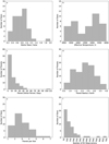 |
Fig. 1 Histograms showing the properties of the stars and planets in our sample: (a) Stellar mass. (b) Stellar effective temperature. (c) Planet orbital period. (d) Planet radius. (e) Multiplicity (number of planets per star). (f) Number of RV observations per system. |
3 HARPS observations
For our analysis, we used RV measurements and activity indicators from the HARPS spectrograph, which are based on publicly available reduced data from the ESO archive, as described in Barbieri (2023). Single-sentence paragraphs are not permitted and must be joined to one or other of the surrounding paragraphs. HARPS is a stabilised high-resolution spectrograph with a resolving power of 110 000, and is capable of sub-m s−1 RV precision for bright, slowly rotating stars. The instrument is mounted on the ESO 3.6 m telescope at the La Silla Observatory in Chile. The observations used in this study all use the high-accuracy mode with a 1 arcsec science fibre on the science target. The second fibre can be used for simultaneous wavelength calibrations. The stars in this sample span a wide range of magnitudes and thus exposure times from a few minutes up to an hour.
The data available through the ESO archive have been processed using the online HARPS pipeline (Pepe et al. 2002), which includes the extraction of 2D spectra that are flux corrected to match the slope of the spectra across echelle orders. RV information is extracted from the spectra by cross correlating with a binary mask that matches the stellar type of the star (Baranne et al. 1996). The S/N cut at 25 enforced when cross referencing with the list of small, known planets from the NASA Exoplanet Archive means that most RVs have precisions of 1–5 m s−1. The median RV uncertainty of this entire dataset is 1.7 m s−1, but this increases up to 12.2 m s−1 for some systems. We note that a few individual data points appear to have very large uncertainties; it is possible that their S/N is incorrectly labelled in the database and so they are not removed by the cut on S/N as they should be; however these do not significantly affect our results. In the later analysis, we use activity indicators based on the cross-correlation function (CCF). These are the bisector inverse slope (BIS) and full width at half-maximum (FWHM). We use these activity indicators as we find these are more robust for the largest sample of spectra than chromospheric activity indicators, such as Ca II H&K, and Hα, which may be more sensitive to low data fidelity.
The only additional step to the data collection was to also do a sigma-clip on the RV data. We used the astropy sigma-clip tool to cut out any RVs more than 3 sigma away from the median, with a maximum of two iterations of this. This finds the median and standard deviation of the data and then removes points that are more than three standard deviations above or below that median value. This is done for two iterations. For most targets, the sigma-clipping does not remove any data because the standard deviation is large anyway. For a few targets with many (>500) observations, it does remove more observations, but still leaves most for the modelling. For one single target, we have only 49 RV observations left after sigma-clipping, this is below our original threshold of 50 epochs, but we chose to include it in the sample anyway.
For a few targets, we also needed to remove specific data points that were clear outliers; see Appendix A.1 for details of this. After the sigma-clipping and removal of data for specific targets, we are left with 6428 individual RV observations. The baseline of observations ranges from approximately 60–6700 days, with a median baseline of around 600 days. The full data used for the final fits for all targets are available online.
It is becoming increasingly common in RV analysis to use GPs to help mitigate the effects of stellar activity (e.g. Haywood et al. 2014; Grunblatt et al. 2015). One promising way to do this is a multidimensional GP, where you fit both the RV data and some activity indicators simultaneously (for an explanation of this process, see e.g. Barragán et al. 2019b; Aigrain & Foreman-Mackey 2023). There are a range of different activity indicators that can be used. In our analysis, we chose to include some of the most commonly used ones: the FWHM and the BIS.
While we have chosen to use HARPS data to ensure the consistency in the RV instrument used, given the long time HARPS has been observing, there are some offsets in the data. In particular, the HARPS fibre was upgraded in 2015, causing a possible RV offset. It is recommended to account for this shift by modelling the HARPS pre-upgrade data as if they were from a different instrument from that providing the HARPS post-upgrade data. For this reason, we label all RV data as either ‘HARPS_pre’ or ‘HARPS_post’. Within the modelling, we set these as two separate instruments – meaning we account for an offset between them. In most cases, the data are all after the upgrade, but in a few cases, the data are from before the upgrade or are a mixture of pre- and post-fibre-upgrade data.
4 Automating the process
One of the biggest challenges of this project was in the initial setup of the RV modelling. We wanted to move away from an ‘artisanal’ approach of looking at one system at a time, to automating a process to model many systems at once. This is for two reasons: we want our method to be generally applicable to any system; and we did not want to introduce any biases by manually setting the priors and input parameters.
To overcome this, we first query the NASA archive to find the required parameters for each individual target: the stellar mass, radius, and temperature, and the planet period, transit midpoint, radius, and mass. We use the composite parameters table from the archive for these values. The planet orbital period and transit midpoint (for non-transiting planets, this parameter has the same name but refers to the time of conjunction) are used as priors in our RV modelling. The other parameters are used for comparison in our results and discussion, but are not used directly in the modelling. We separate the HARPS archive data into individual files for each star, applying our sigma-clipping and removal of specific data where necessary. For each model, we create an input file for the fitting toolkit that can be used for all targets; that is, we have one input file per model, as opposed to having one per target. This significantly reduces the time needed to set up each model run.
5 Radial velocity modelling choices
Distinguishing between planetary and stellar signals in RV data remains a challenge in exoplanet detection. The task is particularly difficult when dealing with active stars, where stellar activity can produce RV signals that mimic or obscure those of orbiting planets. Gaussian processes have emerged as one of the most powerful tools for addressing this issue. GPs offer a highly flexible and non-parametric approach to modelling complex stochastic variations, such as those induced by quasi-periodic stellar activity using tailored quasi-periodic kernels (see Aigrain & Foreman-Mackey 2023).
The benefits of using GPs extend beyond their flexibility. They can incorporate prior knowledge about the system, such as the expected periodicity of stellar activity, and can be combined with other models to account for additional physical processes. This adaptability makes GPs particularly well-suited for analysing spectroscopic time series of active stars, where traditional methods often struggle. Indeed, numerous studies have demonstrated the effectiveness of GPs and their variants – such as multidimensional GPs – in identifying RV signals of planets in the presence of significant stellar activity (see Rajpaul et al. 2015; Barragán et al. 2022). The multidimensional variant of GPs has demonstrated its effectiveness in enhancing the precision of planetary detection, particularly in scenarios where activity indicators provide significant information about the underlying stellar signals (see Barragán et al. 2023). This approach leverages the underlying relation between RV data and activity indicators, allowing for a more accurate separation of planetary and stellar signals. However, the advantages of this multidimensional GP framework diminish under certain conditions. Specifically, when the data suffer from suboptimal sampling or are dominated by large amounts of white noise, the activity indicators may fail to capture information about the stellar signals. In such cases, the use of a multidimensional GP does not offer any significant improvement over traditional methods, as the lack of reliable activity information limits the framework’s ability to accurately model the stellar signal (see Barragán et al. 2024).
A commonly employed kernel that allows stochastic periodic behaviour to be modelled is the quasi-periodic (QP) kernel (as introduced by Roberts et al. 2013), defined as
![Mathematical equation: $\[\gamma_{\mathrm{QP}}(t_{i}, t_{j})=A^{2} \exp \left\{-\frac{\sin ^{2}\left[\pi\left(t_{i}-t_{j}\right) / P_{\mathrm{GP}}\right]}{2 \lambda_{\mathrm{p}}^{2}}-\frac{\left(t_{i}-t_{j}\right)^{2}}{2 \lambda_{\mathrm{e}}^{2}}\right\},\]$](/articles/aa/full_html/2025/01/aa52127-24/aa52127-24-eq1.png) (1)
(1)
where A, the amplitude, is a parameter that works as a scale factor that determines the typical deviation from the mean function, PGP represents the characteristic periodicity of the GP, λp denotes the inverse of the harmonic complexity (indicating the complexity within each period), and λe represents the timescale of long-term evolution.
Once we have our data files for each system, we then have to choose how we model the RVs to find the planet masses. We chose to use the package Pyaneti (Barragán et al. 2019b, 2022) for all of our modelling, as it offers a variety of options for the fitting and is partly written in fortran90, meaning it runs much faster than an entirely Python-based code. Pyaneti is also a fairly common choice of package within the RV modelling community and makes use of multidimensional GPs (Rajpaul et al. 2015; Jones et al. 2017; Gilbertson et al. 2020) to mitigate stellar activity. For a full description of how pyaneti implements the QP kernel described in Eq. (1) within the multi-GP framework, see Barragán et al. (2022). Other RV fitting toolkits that make use of multidimensional GPs include PyORBIT (Malavolta et al. 2016, 2018) and S+LEAF (Delisle et al. 2022). In addition to our goal of providing a homogeneously derived sample of small planet masses, we also wanted to investigate how the choices in modelling affect the derived planet mass. For this reason, we chose to run 12 different models on the data. We wanted to compare the impact of using a GP versus no GP; the dimension of GP used; adding a long-term trend parameter; and modelling orbits as circular or eccentric. See Table 1, which outlines all the models we used.
For all runs, we performed Markov chain Monte Carlo (MCMC) samplings using the sampler included in pyaneti, which is based on an ensemble sampler (Foreman-Mackey et al. 2017). We sample the parameter space with 200 Markov chains. Each chain is initiated randomly with values within the prior ranges. We create posterior distributions with the last 1000 iterations of converged chains with a thin factor of 10. This generates distributions with 200 000 independent points per each sampled parameter.
As well as the specific model choices, we also wanted to be consistent in our application of priors for the modelling parameters. We chose to set a Gaussian prior on both the orbital period, P, and time of conjunction, Tc, listed in the NASA archive using the 1σ errors. Typically, these values have been found through transit fitting of the planets. For several systems, there are no listed values of this in the archive, and for these we manually checked the original publications and added in the values ourselves; details of this procedure are provided in Appendix A.2. For all other planetary orbit parameters, we chose to use wide uniform (uninformative) priors. For the eccentricity of the planetary orbit, we set either an eccentricity fixed at zero (for our circular model cases) or parameterised the eccentricity and argument of periastron to
![Mathematical equation: $\[e \omega_{1}=\sqrt{e ~\sin~ \omega_{*}} ~\text{and} ~e \omega_{2}=\sqrt{e ~\cos~ \omega_{*}}.\]$](/articles/aa/full_html/2025/01/aa52127-24/aa52127-24-eq2.png) (2)
(2)
This has the benefit of not truncating at zero, which is often a problem in modelling eccentricities (Lucy & Sweeney 1971). However, after running models including eccentricity, we noticed that, in some cases, a very high eccentricity is found, which seems unlikely for so many systems. This is likely due to the model fitting high-eccentricity orbits to spurious outliers in the data (Hara et al. 2019). For this reason, we also chose to run two additional models (models e and n, as described in Table 1), which put a prior on the eccentricity as a beta distribution. We used the form of Van Eylen et al. (2019) for single-planet systems, as this is the more general case.
For the GP hyperparameters, we again used wide uniform priors. Except in the case of the GP period, PGP, where we set this based on the stellar type. It has been shown that the GP period links strongly to the stellar rotation period (Nicholson & Aigrain 2022). For each star in our sample, we used the published stellar effective temperature and converted this to a B − V magnitude; using the relation from Mamajek & Hillenbrand (2008), we then estimated the maximum stellar rotation period for a given stellar age. Taking the upper limit of 9 Gyr, we assigned maximum rotation periods of 60, 50, 40, and 20 days for stars with temperatures of <4000 K, 4000–5000 K, 5000–6000 K, and >6000 K, respectively. We also then set the maximum timescale of evolution of active regions, λe, to be twice this rotation period. We note that future work may benefit from using more physically motivated GP hyperparameter priors based on stellar type and age.
The choice of priors for the multi-GP amplitudes was informed by the results of previous analyses that reflect the underlying correlations between the RVs and the CCF-derived activity indicators. (e.g. Barragán et al. 2019a, 2022, 2023). Specifically, previous studies observed that when the RV amplitudes (A0 and B0 are positive, the corresponding amplitudes for the FWHM are also positive, while those for the BIS are negative. For this reason, we set A0 and B0 to be positive, and left the amplitudes for the other hyper-parameters to vary more freely.
Overview of the 12 models applied to RVs and activity indicators in this study.
6 Results and discussion
We remodelled 6428 HARPS RV measurements for 44 stars harbouring 87 small, transiting planets. In this section, we summarise our findings and analyse the impact of model choice when fitting RV signals. For three of our targets, TOI-269, TOI-4399, and HD 3167, our models cannot provide a good fit to the available data. TOI-269 is an active M dwarf star where a custom RV extraction was used in the discovery paper alongside additional photometric data to provide a good fit (Cointepas et al. 2021). TOI-4399 is a very young star with strong activity signals and no published mass measurement (only an upper limit, Zhou et al. 2022). Our modelling suggests that additional data are required for this system in order to fully characterise the planetary mass. HD 3167 has only 50 RV observations but is a four-planet system, which leaves only a low degree of freedom when fitting more than 20 parameters, depending on the model choice. When modelling this system with a GP, this issue is amplified and the degrees of freedom are too few to fit the data well. For the following sections, we remove these three target stars from our analysis, resulting in a total of 83 small planets orbiting 41 stars. For completeness, the final results tables include the fits for these three planets.
The extracted RV amplitude, eccentricity, Bayesian information criterion (BIC), and the Akaike Information Criterion (AIC) for all models for each planet are shown online in Table B.1. The full posterior distributions and plots of each system, plus the full list of best-fit parameters and GP hyperparameters, are available online. The masses given in the ‘params’ file in these full results online should be interpreted as an m sin i value, and we note that the stellar parameters used to calculate these are from the default NASA Exoplanet Archive table, meaning they are heterogeneous in nature themselves. Paper II will provide a more homogeneous set of planet masses using a consistent stellar characterisation method. Here we summarise the main findings by comparing the impact of different modelling choices.
Priors used for all parameters in all models.
6.1 Impact of long-term trends
We compare the extracted K amplitude (RV amplitude) for each target with the different models. Panel a of Figure 2 shows the extracted K amplitude for the three models a–c, which have no GP added to mitigate stellar activity. The difference between the models is that model b has a long-term linear trend added, model c has a long-term quadratic trend added, and model a has no long-term trend. The purpose of adding a long-term trend in RV modelling is typically to account for potential changes in the instrument or telescope over long baselines, or to account for the impact of a longer-period unknown planet (or star) in the system (e.g. Espinoza et al. 2019; Korth et al. 2023). In some cases, a significant measurement of a long-term trend in RV data has been used to claim the discovery of a planet candidate (Lubin et al. 2022). We wanted to test whether adding a model of a long-term trend to all systems – regardless of whether we think there is a potential for an additional planet – makes a difference to the extracted RV amplitude. Panel a of Fig. 2 shows that the addition of any long-term trend makes only a very small difference to the K amplitude found for most targets. This is likely because no trends are evident in the data for these targets. However, in a few cases, a more noticeable difference is seen, and although the error bars typically overlap, the median amplitude found can vary by 1 m s−1 or more. The difference between a linear and quadratic long-term trend is very minor, and the 1σ error bars overlap almost completely for all planets.
In panel b of Fig. 2, we show a histogram of the root mean squared (RMS) of the residuals for the three models a–c. The highest RMS of residuals is for model a, with no long-term trend added. The overall distribution is very similar for all three models.
Panel c of Figure 2 shows a histogram of the difference in RV amplitude of our models compared to the most simple model; that is, the RV amplitude for model c minus the RV amplitude for the same planet for model a. In both the linear and quadratic trend cases, the distribution centres around 0 m s−1, and almost all targets have a difference within ±1 m s−1.
The amplitude of the trend itself for both the linear and quadratic cases is shown in panel d of Fig. 2. We note that the quadratic trend case has been multiplied by 1000 to allow it to be visible on the same axes. For the linear case first (model b), the amplitude of the trend is below 0.20 m s−1 days−1 in all cases, with most targets exhibiting a value of lower than 0.05 m s−1 days−1. For the quadratic trend case, all targets have trend amplitudes of below 0.35 ×10⁻³ m s−1 days−2, with almost all targets showing values of less than half this amount. Based on these results, the indiscriminate addition of a long-term trend to the model does not make a significant difference on the planet mass found because the amplitude of the trend is very small.
Finally, in panel e of Fig. 2, we show the distribution of RV amplitude uncertainties for the three models a–c. The peak of the distribution in all cases is around 0.6 m s−1, with the highest uncertainties being of around 5 m s−1. The difference between the three models is not significant, and it is likely that the systems in our sample do not have an external high-mass companion, or that the RV observations we have are not sensitive to the long-term trend.
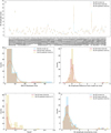 |
Fig. 2 Impact of long-term trends. Panel a: comparison of the RV amplitude found for each target for three different models, a–c. Error bars show the 1σ uncertainty from the MCMC posteriors. Target names are given as TIC IDs with the letter of the planet. Panel b: histogram showing the root-mean-squared error of the residuals to the fit. Panel c: histogram showing the RV amplitude found compared to model a. Panel d: histogram showing the amplitude of the trend found (for the linear trend in m s−1 days−1, for the quadratic trend in m s−1 days−2). The asterisk marks cases where the value for the quadratic trend amplitude has been multiplied by 1000 to plot on the same axes. Panel e: histogram showing the 1σ uncertainty in the RV amplitude found for the different models. |
6.2 Impact of eccentricity
When investigating how modelling orbits as circular or eccentric impacts the planet masses found, we take the no-GP model and either set a uniform eccentricity prior, model d, or we set the prior on eccentricity in the form of a beta distribution, model e. Both of these cases are described in Sect. 5. Figure 3 shows the results of these models compared to the circular case (model a).
In panel a of Fig. 3, we show how the RV amplitude changes for the three models for each planet in our sample. For some very small planets, the eccentric case gives an RV amplitude that is significantly different from the circular or beta distribution case; for example for TIC 437444661 d, and TIC 4610830 f. Even for planets where the 1σ error bars overlap, the difference in the median value of RV amplitude varies by as much as a factor of 3; for example, for TIC 428829990 d, it ranges from approximately 2 m s−1 to 7 m s−1. For all planets, the circular and beta-distribution models, that is, a and e, give the most similar results, with d, the eccentric case, giving the most different ones. Panel b in Fig. 3 shows the RMS of the residuals for the three models. The distributions for all three models are very similar, with no significant differences between them.
When comparing the RV amplitude found for models d and e to that found for model a, as shown in panel c of Fig. 3, we find that a uniform prior on the eccentricity (model d) gives, on average, higher values of RV amplitude, and therefore higher planet masses. For this eccentric case, the RV amplitude difference is found to be slightly offset from 0 m s−1 and has a much wider range, up to around ± 6 m s−1. For the beta distribution case, model e, the amplitude difference centres around 0 m s−1 and has a much smaller range of values, with almost all planets showing a less than 1 m s−1 difference in RV amplitude compared to the circular case. The model with a beta distribution on eccentricity gives much more similar RV amplitudes to the circular case, whereas the uniform prior on eccentricity gives higher RV amplitudes on average. This highlights the importance of choosing the prior on eccentricity with care.
We also performed this analysis for the 3D GP models, which have different eccentricities: the circular case (model k), the case with a uniform prior on eccentricity (model m), and the case with a beta distribution on eccentricity (model n). We find very similar results: the beta distribution gives the most similar results to the circular case. The model with a uniform prior on eccentricity tends to find higher RV amplitudes on average.
The distributions of eccentricity values found for the models with a uniform prior on e (model d) and a beta distribution (model e) are shown in panel d of Fig. 3. For model d, the distribution is almost flat, with eccentricity values ranging all the way up to 0.9. For the beta distribution case, model e, the eccentricities found centre close to zero, with the highest value being 0.2, fairly closely following the prior distribution set. Given the very high values of eccentricity found in the case for model d, we wanted to check that the wide priors set on the RV amplitude were not contributing to this. We ran model d again for all targets but restricted the RV amplitude to be less than 50 m s−1. We found that the eccentricity and RV amplitude did not change by more than 1% in any case, and so the wide priors on RV amplitude are not the reason for the high eccentricities. In some ways, it is surprising to find such high values of eccentricity, especially as we chose to parametrise the eccentricity and argument of periastron as in Eq. (2), which should help with this issue. It is possible that the model is finding such high eccentricities due to spurious data points (Hara et al. 2019).
Finally, panel e of Fig. 3, shows the RV amplitude uncertainty for each planet found with models a, d, and e. The circular and beta distribution models, a and e, have the most similar RV uncertainties, both with distributions peaking below 1 m s−1 and only a few higher outliers. For the eccentric case, model (d), the distribution in RV amplitude uncertainty peaks at a higher value and has higher outliers of up to 7 m s−1.
Based on our results, it is clear that using a uniform prior on eccentricity is not a suitable approach for modelling large sets of RV data. Instead, we suggest using an informative prior distribution on the eccentricity, such as a beta distribution. We note that the RV amplitude (and therefore planet mass) found for the whole sample does not change much between simply fixing the orbits as circular and using a beta distribution in eccentricity. However, we believe that the use of a beta distribution is more physically motivated, as we would not expect every planet in our sample to be on a perfectly circular orbit. Alternatively, the simultaneous modelling of photometric data may help accurately constrain the eccentricity, though testing this in more detail is beyond the scope of this paper.
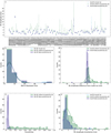 |
Fig. 3 Impact of orbital eccentricity. Panel a: comparison of the RV amplitude found for each target for three different models, a, d, and e. Error bars show the 1σ uncertainty from the MCMC posteriors. Target names are given as TIC IDs with the letter of the planet. Panel b: Histogram showing the RMS error of the residuals to the fit. Panel c: histogram showing the RV amplitude found compared to model a. Panel d: histogram showing the value of eccentricity found. Panel e: histogram showing the 1σ uncertainty in the RV amplitude found for the different models. |
6.3 Impact of GP dimension
We compare the K amplitude found with different dimensionalities of GP: no GP, model a; a 1D GP (fitting just to the RVs), model f; a 2D GP (fitting to the RVs and an activity indicator, in this case the FWHM), model h; and a 3D GP (fitting to the RVs and two activity indicators, in this case FWHM and BIS), model k. In all cases, the models are for a circular orbit.
Figure 4 shows the results of these four models with different dimensions of GP. In panel a we compare the extracted RV amplitude for all planets in our sample with the different models. There are two things of note: the biggest error bars tend to be from the no GP case, and the biggest differences also tend to be for the no GP case. However, for nearly all the planets in the sample, the dimension of the GP does not significantly change the extracted RV amplitude. Although we note that the median value of RV amplitude for a given planet indeed does vary a little between the models, which would have an impact on statistical studies of the population.
Panel b of Fig. 4 shows the RMS of the residuals for the four models. All the GP models have very similar distributions, with the no GP case having the largest RMS values. Therefore, the inclusion of a GP indeed reduces the RMS of the residuals on average.
Panel c of Fig. 4 shows the difference in RV amplitude found for each model compared to the no GP case. Here, there is a slight shift seen for the 1D GP case compared to the 2D and 3D cases. The 1D GP case finds slightly higher RV amplitudes on average, and is most different from the other GP models.
Panel d of Fig. 4 shows the difference in RV amplitude found for the 2D and 3D GP models compared to the 1D GP case. The 2D and 3D GP models overlap very well in terms of RV amplitude. They both show some differences from the 1D GP model (which would be at zero in this plot). The 1D GP model is the most inconsistent of the three models.
Finally, in panel e of Fig. 4, we show the uncertainty in the RV amplitude found for every planet with each model. All models have a peak in uncertainty at below 1 m s−1. The no GP case has a slightly shifted peak uncertainty and also has the highest outliers. The models including a GP show a very similar distribution in RV amplitude uncertainty.
Based on these results, if using a GP, we would recommend using a multidimensional GP that fits to an activity indicator. This is because the 2D and 3D GP results seem the most robust compared to the 1D case; the 1D GP model find the biggest difference in RV amplitude.
6.4 Model comparison
We compared each of our models by computing the BIC and the AIC. Table B.1 gives the value of each of these for each model of every system. However, we note that none of these metrics are perfect indicators of goodness of fit, and additionally, the use of different data sets (in the case of the 2D and 3D GP models) means that you cannot directly compare these metrics. Regardless, we provide this information as an overview. For the models that use only the RV data, the lowest AIC model for 78 planets is the 1D GP circular model f, followed by the 1D GP model with a uniform prior on eccentricity g for 11 planets. The remaining planets all prefer a no GP model. For the 2D GP models, 85 planets prefer the circular model h over the uniform prior eccentric model j. For the 3D GP case, 80 planets prefer the circular case k, 18 the eccentric model with beta distribution n, and 15 the uniform eccentric model n. In general, the circular models seem to be preferred by the AIC, possibly because these have fewer parameters and so are not penalised by the goodness-of-fit metrics; though in some cases the non-circular models are still preferred.
To define our ‘best’ model for the adopted set of planet parameters for each target, we first find the lowest AIC model from the models that use only the RV data (models a to f). If the best model for a given target corresponds to the 1D GP model, we take this as an indication that a GP is required for that specific target. For the targets that require a GP, we assign the 3D GP with beta distribution as the best model. For the targets that prefer a no GP model, we assign the no GP beta distribution model as the best model.
We note that the beta distribution models do not always give the ‘best’ fit in terms of AIC and BIC. However, we choose these as our final models as the treatment of eccentricity is the most realistic: not all planets in our sample will be on circular orbits, and using a uniform prior for eccentricity gives spuriously large eccentricity values. Additionally, the beta distribution is an empiric result based on transit observations of small planets and so has good physical motivation (Van Eylen et al. 2019). We chose the 3D GP case rather than the 1D or 2D case because the 1D GP case appears to be the least consistent with the others (in terms of extracted RV amplitude), and because the 3D GP case makes use of the most information – in the form of the FWHM and BIS indicators. We note that the 3D GP model will always have a lower value of AIC compared to the 2D GP case because it has more data points, but this is not why we chose this model. The fitted planet parameters for the best model chosen for each target are shown in Table B.2.
Panel a of Fig. 5 shows the RV amplitude of the best model for each planet in our sample compared to the default published value from the NASA Exoplanet Archive (though we note that some planets do not have a published RV amplitude, and that for many of those that do have one, the data are different from those used here). For some planets, there is a significant difference between the two. Even where the 1σ error bars overlap, the difference in the median RV amplitude for a given planet can vary by up to a factor of 2. This would have a big impact on the calculated bulk density of the planet and therefore change the estimated composition.
In panel b we show a histogram of the RV amplitude differences from our best model compared to the default published values (for targets that have this published value). The distribution here does peak around 0 m s−1; however, some targets have difference in amplitude of up to 5 m s−1. On the one hand, this is reassuring as it seems that our results are broadly consistent with the literature. On the other hand, there are still differences seen for some targets, which would have an impact on the overall demographics of this sample. This highlights the need for a homogeneous analysis approach if we want to study populations of planets rather than individual systems.
Finally, in panel c we present a histogram of the RV amplitude uncertainties for our best model compared to those of the default published amplitudes. It is clear that these latter amplitudes have a lower uncertainty on average compared to our best model. We discuss why this may be the case in Sect. 7 (most likely due to additional data being used in the published works) and note that the aim of this work is not to find the most precise planet masses, but rather to provide a sample where the masses have been found homogeneously. Overall, this comparison shows that a homogeneous approach finds a different distribution in RV amplitudes for some targets (and therefore planet mass) compared to a heterogeneous sample.
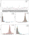 |
Fig. 4 Impact of GP dimension. Panel a: comparison of the RV amplitude found for each target for four different models, a, f, h, and k. Error bars show the 1σ uncertainty from the MCMC posteriors. Target names are given as TIC IDs with the letter of the planet. Panel b: histogram showing the RMS error of the residuals to the fit. Panel c: histogram showing the RV amplitude found compared to model a. Panel d: histogram showing the RV amplitude found for models h and k compared to model f. Panel e: histogram showing the 1σ uncertainty in the RV amplitude found for the different models. |
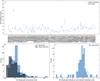 |
Fig. 5 Panel a: RV amplitude found with the best model for each planet in our sample (blue stars) compared to the default published value from the NASA Exoplanet Archive (grey squares). Some planets do not have a published RV amplitude on the archive. Panel b: histogram showing the RV amplitude of our best model for each planet subtracted by the default published value. Panel c: histogram showing the RV amplitude uncertainty for our best model compared to the uncertainties of the default published amplitudes. |
6.5 TIC 98720809: A representative example
In this section, we show the full results for one example, TIC 9870809, a two-planet system that has a very consistent RV amplitude found across all models with a GP. For this target, we take the 120 HARPS RV observations (all post-fibre-upgrade) and the priors found from the NASA Exoplanet Archive composite parameters table. This gives the priors listed in Table A.2.
Our best model for this target is the 3D GP model with beta distribution on the eccentricity, and we focus on that specific case here. After the MCMC fitting, we find the parameters given in Table A.3. Figure 6 shows the full time series data for this target, with the best-fit model shown for the 3D GP with beta distribution on eccentricity case. The impact of the GP is clear in this plot: the planet signal alone would not reproduce the observations well without an activity model. In Figs. 7 and 8 we show the phase-folded RV data with best-fit model (including the GP) for planets b and c, respectively. Finally, the full posterior distribution found for all fitted parameters is shown in Fig. A.1.
As a comparison, we now show the result plots for this same target but without a GP added to mitigate stellar activity. Specifically, we show the no GP model with a beta distribution on eccentricity, so that we can directly compare. In Fig. 9 we show the time-series data with this no GP model; the data are very clearly not well fitted by this model, demonstrating the positive effect of the addition of a GP in this case. In Figs. 10 and 11, we show the phase-folded RV data with best-fit model (including the GP) for planets b and c, respectively. Again, it is clear that this model does not fit the data well, and in this case the planet signals would not be recovered. Finally, Fig. A.2 shows the full posterior distribution of fitted parameters for this no GP model. In this case, the RV amplitude found for both planets is not significant; that is, it is within 1σ of 0 m s−1 and so using only this model with these data would result in non-detections for both planets.
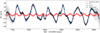 |
Fig. 6 Best-fitting two-planet orbital model for TIC 9870809. HARPS data shown by blue circles as a function of time. The best-fitting model for the planet signals is shown in red, the 3D GP model in blue, and the combined planets and GP shown in black. The dark and light shaded areas show the 1σ and 2σ credible intervals of the corresponding GP model, respectively. |
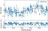 |
Fig. 7 Phase-folded RV data from HARPS (blue circles) alongside the best-fitting planet model for TIC 9870809 b (with the effect of the other planet and the GP model subtracted). The lower part shows the residuals from the fit. There appears to be no trends visible in the residuals. |
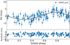 |
Fig. 8 Phase-folded RV data from HARPS (blue circles) alongside the best-fitting planet model for TIC 9870809 c (with the effect of the other planet and the GP model subtracted). The lower part shows the residuals from the fit. There appears to be no trends visible in the residuals. |
7 Caveats and recommendations
This work presented a number of challenges, which are mostly related to the use of archival data. Barbieri (2023) discusses the possibility that some data and/or targets are potentially missing from our sample, which could impact the RV amplitudes found. We also note that we did not reprocess the raw observations to find the RVs ourselves; this would likely reduce some of the challenges we faced and could be a useful additional step in future work.
Another difficulty with using archival data is that we have no control of the observing strategy. In some cases, the cadence and baselines of observations for a target are not ideal for fitting GPs. Having long gaps between seasons of data makes it harder for the GP to capture the stellar activity signal. In future we recommend teams to think about trying to reduce the length of the gaps between their observing seasons where possible. We also recommend that large RV surveys be designed to mitigate the biases inherent to the observing strategy where possible, following the work of Teske et al. (2021) for example.
Another caveat of our results is that we used only the RVs available from HARPS. For some of our targets, there are additional data available from other RV instruments. In some cases, this means that the published K amplitudes are more precise than the ones we have found in our work. We would recommend that future studies investigate the impact of adding additional data.
Finally, we note that some activity indicators or combinations of indicators may be more capable of mitigating different manifestations of stellar activity than others. The typical activity seen in an M dwarf star is not the same as a G type star, and so having a one-size-fits-all approach may not be the most effective. However, the aim of this work is not to provide the ‘best’ RV amplitude for each small planet, but is instead to create a database of homogeneously derived planet parameters that can be used for demographics studies.
Based on the experience of this experiment, we propose a general set of recommendations for observing and modelling RVs of planet hosting stars in large batches:
Avoid having multiple seasons of observations with large (>1 year) gaps in between if a GP is required to mitigate stellar activity signals.
Avoid modelling orbits as eccentric without a prior on the eccentricity (e.g. in the form of a beta distribution).
If using a GP, it should be used in combination with at least one activity indicator.
Using a heterogeneously derived sample of planet masses will likely induce some biases when looking at a large sample: to complete demographics studies, we recommend modelling planet masses in a homogeneous way.
As a community, we should collate a database of homogeneously derived masses wherever possible.
Plenty of work still needs to be done to understand the importance of homogeneous mass analysis in exoplanets. In future work, it will be beneficial to look at: the impact of how the RVs are extracted from the spectra; the potential systematic difference between the RV fitting toolkits; and the degree to which a joint fit with photometry changes planet masses. We also note that it would be important to test the robustness of the RV amplitude found when changing the priors on the GP and also the choice of GP kernel, particularly for different stellar types.
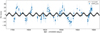 |
Fig. 9 Planet model with no GP beta distribution on eccentricity for TIC 9870809. HARPS data shown by blue circles as a function of time. The best-fitting model for the planet signals is shown in black. The model does not fit the data well. |
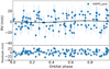 |
Fig. 10 Phase-folded RV data from HARPS (blue circles) alongside the planet model with no GP beta distribution on eccentricity for TIC 9870809 b (with the effect of the other planet subtracted). The planet signal is hardly visible. |
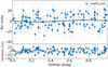 |
Fig. 11 Phase-folded RV data from HARPS (blue circles) alongside the planet model with no GP beta distribution on eccentricity for TIC 9870809 c (with the effect of the other planet subtracted). The lower part shows the residuals from the fit. The planet signal is hardly visible. |
8 Conclusions
In this work, we re-fitted all publicly available HARPS RV observations for 44 stars hosting small planets with a planet radius of smaller than 4 R⊕. For each target system, we used 12 different models to investigate how model choice impacts the planet mass found.
We find that the addition of long-term trends to the model (either linear or quadratic in nature) makes a difference in some specific cases but that overall this model choice has only a very small impact. Almost all targets have an RV amplitude within 1 m s−1 of that found with a model with no trend.
The impact of eccentricity is much more significant. We find that the RV amplitudes found for fixed circular orbits differ (in some cases significantly) from those found for orbits that are modelled as eccentric with wide uniform priors. We recommend using a prior on the eccentricity, such as the beta distribution presented in Van Eylen et al. (2019) to ensure that the model does not find very high values of eccentricity.
Finally, we find that the addition of a GP, and in particular a multidimensional GP that fits on RVs and activity indicators, indeed impacts the mass found. On average, the RV amplitude found is within 1 m s−1 of that found for the no GP case; however this can vary by up to more than 6 m s−1. The 1D GP model, fitted just on the RVs, is the most different from the others. Therefore, we recommend using either a 2D or a 3D GP model for active stars. A 3D GP model takes longer computationally and so a 2D GP may be better where time is restricted and/or many targets need to be modelled.
Overall, our results demonstrate the importance of considering homogeneity in the analysis of RV observations to find planet masses. This will be particularly important for future surveys, such as the PLATO mission, which aims to provide a catalogue of accurate and precise planet parameters for many new systems. To ensure this sample is accurate at the population level, it will be necessary for the analysis to be done in a homogeneous way.
In Sect. 7 we describe some of the caveats of our work. In particular, we note that the RV amplitudes found in this work may not be the most precise for each individual planet in the sample. Rather, our aim is to provide a sample of masses determined homogeneously. We also note that future work should investigate the impacts of different models for different stellar types, and whether a joint model with photometric data would be of benefit. In Paper II (Osborne et al., in prep.), we will investigate how the mass–radius distribution changes for our homogeneous sample from that seen for the heterogeneous sample. We will also comment on the future characterisation possibilities of these small planets.
Data availability
All data required to complete the analysis are publicly available on the ESO archive. However we also provide the full list of radial velocities used in our analysis at the CDS via anonymous ftp to cdsarc.cds.unistra.fr (130.79.128.5) or via https://cdsarc.cds.unistra.fr/viz-bin/cat/J/A+A/693/A4.
The full results table, Table B.1 is available at https://zenodo.org/records/14170646, and the best model results table, Table B.2 is available at https://zenodo.org/records/14215941.
Acknowledgements
We thank the anonymous referee for their constructive and insightful suggestions. H.L.M.O. would like to thank the Science and Technology Facilities Council (STFC) and the European Southern Observatory (ESO) for funding support through PhD studentships. V.V.E. has been supported by UK’s Science & Technology Facilities Council through the STFC grants ST/W001136/1 and ST/S000216/1. This work is based on observations collected at the European Organisation for Astronomical Research in the Southern Hemisphere under ESO programmes: 183.C-0972 192.C-0852, 60.A-9036, 072.C-0488, 198.C-0836, 091.C-0936, 1102.C-0923, 1102.C-0249, 60.A-9700, 0102.C-0584, 096.C-0499, 106.21TJ, 0100.D-0444, 188.C-0265, 198.C-0169, 0100.C-0750, 098.C-0304, 098.C-0739, 0102.C-0451, 0101.C-0510, 192.C-0224, 0103.C-0759, 0102.D-0483, 0102.C-0525, 196.C-1006, 085.C-0019, 087.C-0831, 096.C-0460, 1102.C-0249, 1102.C-0249, 60.A-9709, 1102.C-0923, 0103.C-0442, 0103.C-0874, 1102.C-0339, 183.C-0437, 1102.C-0339, 082.C-0718, 0100.C-0808, 099.C-0491, 0101.C-0788, 0103.C-0548, 0102.C-0338, 0101.C-0829, 0104.C-0413, 105.20N0, 198.C-0838, 191.C-0873, 095.C-0718, 0100.C-0884, 283.C-5022, 098.C-0860, 097.C-0948, 074.C-0364, 0101.C-0497, 0101.C-0407, 282.C-5036, 082.C-0308, and 088.C-0323. All data is publicly available on the ESO archive. We thank the PIs of the programmes: Udry, Mayor, Diaz, Gandolfi, Armstrong, Demedeiros, Lorenzo-Oliveira, Melendez, Santerne, Ehrenreich, Lagrange, Benatti, Berdinas, Lo Curto, Nielsen, Bonfils, Allart, Trifonov, Brahm, Albrecht, Astudillo, NIRPS GTO Team, and Robichon. We also thank the many people involved in the observing and archiving of the data, without whom this work would not have been possible.
Appendix A Individual systems
We aimed in all cases to treat the data homogeneously for every target so that the same steps could be applied to everything automatically. However, in a few cases we noticed some issues with individual systems which required us to make manual changes to the input files for those. We tried to keep everything else homogeneous in our analysis, and in most cases it just involved excluding some of the RV data points. These specific cases are detailed below.
A.1 Removal of RV data
For the system TIC 173103335, we noticed that quite a bit of RV data was largely offset (more than 30 km/s) from the rest of the RVs. If we include this data in the fit then the model struggles to find a solution, particularly in the cases including a GP where the additional GP hyperparameters allow for possible over fitting. For this reason, we removed the largely outlying data from this system (we cut out all data with RV values <10km/s. As this is archival data it is difficult to know why in some cases there would be such a large offset; we believe it is likely due to the incorrect stellar mask being applied for the CCF data reduction in the HARPS pipeline.
For TIC 220479565, we again see that this system appears to have some largely offset RV data which makes the modelling very challenging. We choose to cut all data where the RV is negative (i.e. we cut at RV = 0 km/s). In the case of TIC 260004324 we also cut the outlying data points at the threshold of 42.5 km/s. This successfully removes the largely outlying RV data. TIC 56815340 has a large amount of in-transit RV observations, this means that many exposures are taken over the course of one observing night. Because of this, the fitting with a GP takes much longer and can be confused by the many points over one night. For this reason, we remove any data for this target where there are more than 5 observations in a single date.
A.2 Defining priors
For the majority of our targets, the NASA Exoplanet Archive provides details of the orbital period and time of mid-transit, Tc (or time of inferior conjunction for non-transiting companions). However, a few systems do not have Tc listed and so for these we search the published literature for these planets and manually input the values. Table A.1 gives the specific values for these priors and the reference they were taken from. For one system, TIC 280304863, there was no Tc given for planet d, so for this planet we set a wide Gaussian priors on the Tc for planet c.
The Tc values added manually for targets where the NASA Exoplanet Archive does not provide these.
Priors used for the 3D GP model with beta distribution on eccentricity for TIC 9870809.
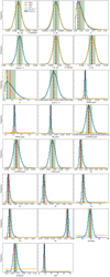 |
Fig. A.1 Full posterior distribution of fitted parameters for TIC 98720809 with the 3D GP beta distribution model. |
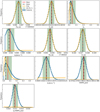 |
Fig. A.2 Full posterior distribution of fitted parameters for TIC 98720809 with the no GP beta distribution model. |
Appendix B Stellar IDs observation summary
The different identifiers of all stars in our sample.
References
- Aigrain, S., & Foreman-Mackey, D. 2023, ARA&A, 61, 329 [NASA ADS] [CrossRef] [Google Scholar]
- Baranne, A., Queloz, D., Mayor, M., et al. 1996, A&AS, 119, 373 [NASA ADS] [CrossRef] [EDP Sciences] [Google Scholar]
- Barbieri, M. 2023, arXiv e-prints [arXiv:2312.06586] [Google Scholar]
- Barragán, O., Aigrain, S., Kubyshkina, D., et al. 2019a, MNRAS, 490, 698 [Google Scholar]
- Barragán, O., Gandolfi, D., & Antoniciello, G. 2019b, MNRAS, 482, 1017 [Google Scholar]
- Barragán, O., Aigrain, S., Rajpaul, V. M., & Zicher, N. 2022, MNRAS, 509, 866 [Google Scholar]
- Barragán, O., Gillen, E., Aigrain, S., et al. 2023, MNRAS, 522, 3458 [CrossRef] [Google Scholar]
- Barragán, O., Yu, H., Freckelton, A. V., et al. 2024, MNRAS, 531, 4275 [CrossRef] [Google Scholar]
- Batalha, N. E., Lewis, T., Fortney, J. J., et al. 2019, ApJ, 885, L25 [Google Scholar]
- Bonfils, X., Almenara, J. M., Cloutier, R., et al. 2018, A&A, 618, A142 [NASA ADS] [CrossRef] [EDP Sciences] [Google Scholar]
- Cadieux, C., Doyon, R., Plotnykov, M., et al. 2022, AJ, 164, 96 [NASA ADS] [CrossRef] [Google Scholar]
- Cloutier, R., Astudillo-Defru, N., Doyon, R., et al. 2017, A&A, 608, A35 [NASA ADS] [CrossRef] [EDP Sciences] [Google Scholar]
- Cointepas, M., Almenara, J. M., Bonfils, X., et al. 2021, A&A, 650, A145 [NASA ADS] [CrossRef] [EDP Sciences] [Google Scholar]
- Collier Cameron, A., & Jardine, M. 2018, MNRAS, 476, 2542 [Google Scholar]
- Cosentino, R., Lovis, C., Pepe, F., et al. 2012, Proc. SPIE, 8446, 84461V [Google Scholar]
- Dai, F., Masuda, K., Winn, J. N., & Zeng, L. 2019, ApJ, 883, 79 [NASA ADS] [CrossRef] [Google Scholar]
- Delisle, J. B., Unger, N., Hara, N. C., & Ségransan, D. 2022, A&A, 659, A182 [NASA ADS] [CrossRef] [EDP Sciences] [Google Scholar]
- Demangeon, O. D. S., Zapatero Osorio, M. R., Alibert, Y., et al. 2021, A&A, 653, A41 [NASA ADS] [CrossRef] [EDP Sciences] [Google Scholar]
- Diamond-Lowe, H., Kreidberg, L., Harman, C. E., et al. 2022, AJ, 164, 172 [NASA ADS] [CrossRef] [Google Scholar]
- Di Maio, C., Changeat, Q., Benatti, S., & Micela, G. 2023, A&A, 669, A150 [NASA ADS] [CrossRef] [EDP Sciences] [Google Scholar]
- Espinoza, N., Hartman, J. D., Bakos, G. Á. et al. 2019, AJ, 158, 63 [Google Scholar]
- Foreman-Mackey, D., Agol, E., Ambikasaran, S., & Angus, R. 2017, AJ, 154, 220 [Google Scholar]
- Fulton, B. J., Petigura, E. A., Howard, A. W., et al. 2017, AJ, 154, 109 [Google Scholar]
- Gibson, S. R., Howard, A. W., Marcy, G. W., et al. 2016, SPIE Conf. Ser., 9908, 990870 [Google Scholar]
- Gilbertson, C., Ford, E. B., Jones, D. E., & Stenning, D. C. 2020, ApJ, 905, 155 [Google Scholar]
- Goffo, E., Gandolfi, D., Egger, J. A., et al. 2023, ApJ, 955, L3 [NASA ADS] [CrossRef] [Google Scholar]
- Grunblatt, S. K., Howard, A. W., & Haywood, R. D. 2015, ApJ, 808, 127 [NASA ADS] [CrossRef] [Google Scholar]
- Gupta, A., & Schlichting, H. E. 2019, MNRAS, 487, 24 [Google Scholar]
- Gupta, A., & Schlichting, H. E. 2021, MNRAS, 504, 4634 [NASA ADS] [CrossRef] [Google Scholar]
- Hara, N. C., Boué, G., Laskar, J., Delisle, J. B., & Unger, N. 2019, MNRAS, 489, 738 [Google Scholar]
- Haywood, R. D., Collier Cameron, A., Queloz, D., et al. 2014, MNRAS, 443, 2517 [Google Scholar]
- Jones, D. E., Stenning, D. C., Ford, E. B., et al. 2017, arXiv e-prints [arXiv:1711.01318] [Google Scholar]
- Klein, B., Aigrain, S., Cretignier, M., et al. 2024, MNRAS, 531, 4238 [Google Scholar]
- Knudstrup, E., Albrecht, S. H., Winn, J. N., et al. 2024, A&A, 690, A379 [NASA ADS] [CrossRef] [EDP Sciences] [Google Scholar]
- Korth, J., Gandolfi, D., Šubjak, J., et al. 2023, A&A, 675, A115 [NASA ADS] [CrossRef] [EDP Sciences] [Google Scholar]
- Lubin, J., Van Zandt, J., Holcomb, R., et al. 2022, AJ, 163, 101 [NASA ADS] [CrossRef] [Google Scholar]
- Lucy, L. B., & Sweeney, M. A. 1971, AJ, 76, 544 [NASA ADS] [CrossRef] [Google Scholar]
- Luque, R., & Pallé, E. 2022, Science, 377, 1211 [NASA ADS] [CrossRef] [Google Scholar]
- Luque, R., Pallé, E., Kossakowski, D., et al. 2019, A&A, 628, A39 [NASA ADS] [CrossRef] [EDP Sciences] [Google Scholar]
- Malavolta, L., Nascimbeni, V., Piotto, G., et al. 2016, A&A, 588, A118 [NASA ADS] [CrossRef] [EDP Sciences] [Google Scholar]
- Malavolta, L., Mayo, A. W., Louden, T., et al. 2018, AJ, 155, 107 [NASA ADS] [CrossRef] [Google Scholar]
- Mamajek, E. E., & Hillenbrand, L. A. 2008, ApJ, 687, 1264 [Google Scholar]
- Mayor, M., Pepe, F., Queloz, D., et al. 2003, The Messenger, 114, 20 [NASA ADS] [Google Scholar]
- McLaughlin, D. B. 1924, ApJ, 60, 22 [Google Scholar]
- Montet, B. T. 2018, Res. Notes Am. Astron. Soc., 2, 28 [Google Scholar]
- Nicholson, B. A., & Aigrain, S. 2022, MNRAS, 515, 5251 [NASA ADS] [CrossRef] [Google Scholar]
- Osborn, H. P., Armstrong, D. J., Adibekyan, V., et al. 2021, MNRAS, 502, 4842 [NASA ADS] [CrossRef] [Google Scholar]
- Osborne, H. L. M., Van Eylen, V., Goffo, E., et al. 2024, MNRAS, 527, 11138 [Google Scholar]
- Otegi, J. F., Bouchy, F., Helled, R., et al. 2021, A&A, 653, A105 [NASA ADS] [CrossRef] [EDP Sciences] [Google Scholar]
- Owen, J. E., & Wu, Y. 2017, ApJ, 847, 29 [Google Scholar]
- Pepe, F., Mayor, M., Rupprecht, G., et al. 2002, The Messenger, 110, 9 [NASA ADS] [Google Scholar]
- Pepe, F., Cristiani, S., Rebolo, R., et al. 2021, A&A, 645, A96 [NASA ADS] [CrossRef] [EDP Sciences] [Google Scholar]
- Polanski, A. S., Lubin, J., Beard, C., et al. 2024, ApJS, 272, 32 [NASA ADS] [CrossRef] [Google Scholar]
- Queloz, D., Bouchy, F., Moutou, C., et al. 2009, A&A, 506, 303 [NASA ADS] [CrossRef] [EDP Sciences] [Google Scholar]
- Rajpaul, V., Aigrain, S., Osborne, M. A., Reece, S., & Roberts, S. 2015, MNRAS, 452, 2269 [Google Scholar]
- Rauer, H., Catala, C., Aerts, C., et al. 2014, Exp. Astron., 38, 249 [Google Scholar]
- Rice, K. 2014, Challenges, 5, 296 [NASA ADS] [CrossRef] [Google Scholar]
- Roberts, S., Osborne, M., Ebden, M., et al. 2013, Phil. Trans. R. Soc. London Ser. A, 371, 20110550 [Google Scholar]
- Rossiter, R. A. 1924, ApJ, 60, 15 [Google Scholar]
- Schwab, C., Liang, M., Gong, Q., et al. 2018, SPIE Conf. Ser., 10702, 1070271 [Google Scholar]
- Teske, J., Wang, S. X., Wolfgang, A., et al. 2021, ApJS, 256, 33 [NASA ADS] [CrossRef] [Google Scholar]
- Thompson, S. J., Queloz, D., Baraffe, I., et al. 2016, SPIE Conf. Ser., 9908, 99086F [Google Scholar]
- Tinetti, G., Drossart, P., Eccleston, P., et al. 2018, Exp. Astron., 46, 135 [NASA ADS] [CrossRef] [Google Scholar]
- Van Eylen, V., Agentoft, C., Lundkvist, M. S., et al. 2018, MNRAS, 479, 4786 [Google Scholar]
- Van Eylen, V., Albrecht, S., Huang, X., et al. 2019, AJ, 157, 61 [Google Scholar]
- Zhou, G., Wirth, C. P., Huang, C. X., et al. 2022, AJ, 163, 289 [NASA ADS] [CrossRef] [Google Scholar]
- Zhu, W., & Dong, S. 2021, ARA&A, 59, 291 [NASA ADS] [CrossRef] [Google Scholar]
According to the NASA Exoplanet Archive Composite Planet Parameters Table Accessed 31-07-2024.
https://exoplanetarchive.ipac.caltech.edu/ Accessed 24-01-2024.
All Tables
The Tc values added manually for targets where the NASA Exoplanet Archive does not provide these.
Priors used for the 3D GP model with beta distribution on eccentricity for TIC 9870809.
All Figures
|
Fig. 1 Histograms showing the properties of the stars and planets in our sample: (a) Stellar mass. (b) Stellar effective temperature. (c) Planet orbital period. (d) Planet radius. (e) Multiplicity (number of planets per star). (f) Number of RV observations per system. |
| In the text | |
|
Fig. 2 Impact of long-term trends. Panel a: comparison of the RV amplitude found for each target for three different models, a–c. Error bars show the 1σ uncertainty from the MCMC posteriors. Target names are given as TIC IDs with the letter of the planet. Panel b: histogram showing the root-mean-squared error of the residuals to the fit. Panel c: histogram showing the RV amplitude found compared to model a. Panel d: histogram showing the amplitude of the trend found (for the linear trend in m s−1 days−1, for the quadratic trend in m s−1 days−2). The asterisk marks cases where the value for the quadratic trend amplitude has been multiplied by 1000 to plot on the same axes. Panel e: histogram showing the 1σ uncertainty in the RV amplitude found for the different models. |
| In the text | |
|
Fig. 3 Impact of orbital eccentricity. Panel a: comparison of the RV amplitude found for each target for three different models, a, d, and e. Error bars show the 1σ uncertainty from the MCMC posteriors. Target names are given as TIC IDs with the letter of the planet. Panel b: Histogram showing the RMS error of the residuals to the fit. Panel c: histogram showing the RV amplitude found compared to model a. Panel d: histogram showing the value of eccentricity found. Panel e: histogram showing the 1σ uncertainty in the RV amplitude found for the different models. |
| In the text | |
|
Fig. 4 Impact of GP dimension. Panel a: comparison of the RV amplitude found for each target for four different models, a, f, h, and k. Error bars show the 1σ uncertainty from the MCMC posteriors. Target names are given as TIC IDs with the letter of the planet. Panel b: histogram showing the RMS error of the residuals to the fit. Panel c: histogram showing the RV amplitude found compared to model a. Panel d: histogram showing the RV amplitude found for models h and k compared to model f. Panel e: histogram showing the 1σ uncertainty in the RV amplitude found for the different models. |
| In the text | |
|
Fig. 5 Panel a: RV amplitude found with the best model for each planet in our sample (blue stars) compared to the default published value from the NASA Exoplanet Archive (grey squares). Some planets do not have a published RV amplitude on the archive. Panel b: histogram showing the RV amplitude of our best model for each planet subtracted by the default published value. Panel c: histogram showing the RV amplitude uncertainty for our best model compared to the uncertainties of the default published amplitudes. |
| In the text | |
|
Fig. 6 Best-fitting two-planet orbital model for TIC 9870809. HARPS data shown by blue circles as a function of time. The best-fitting model for the planet signals is shown in red, the 3D GP model in blue, and the combined planets and GP shown in black. The dark and light shaded areas show the 1σ and 2σ credible intervals of the corresponding GP model, respectively. |
| In the text | |
|
Fig. 7 Phase-folded RV data from HARPS (blue circles) alongside the best-fitting planet model for TIC 9870809 b (with the effect of the other planet and the GP model subtracted). The lower part shows the residuals from the fit. There appears to be no trends visible in the residuals. |
| In the text | |
|
Fig. 8 Phase-folded RV data from HARPS (blue circles) alongside the best-fitting planet model for TIC 9870809 c (with the effect of the other planet and the GP model subtracted). The lower part shows the residuals from the fit. There appears to be no trends visible in the residuals. |
| In the text | |
|
Fig. 9 Planet model with no GP beta distribution on eccentricity for TIC 9870809. HARPS data shown by blue circles as a function of time. The best-fitting model for the planet signals is shown in black. The model does not fit the data well. |
| In the text | |
|
Fig. 10 Phase-folded RV data from HARPS (blue circles) alongside the planet model with no GP beta distribution on eccentricity for TIC 9870809 b (with the effect of the other planet subtracted). The planet signal is hardly visible. |
| In the text | |
|
Fig. 11 Phase-folded RV data from HARPS (blue circles) alongside the planet model with no GP beta distribution on eccentricity for TIC 9870809 c (with the effect of the other planet subtracted). The lower part shows the residuals from the fit. The planet signal is hardly visible. |
| In the text | |
|
Fig. A.1 Full posterior distribution of fitted parameters for TIC 98720809 with the 3D GP beta distribution model. |
| In the text | |
|
Fig. A.2 Full posterior distribution of fitted parameters for TIC 98720809 with the no GP beta distribution model. |
| In the text | |
Current usage metrics show cumulative count of Article Views (full-text article views including HTML views, PDF and ePub downloads, according to the available data) and Abstracts Views on Vision4Press platform.
Data correspond to usage on the plateform after 2015. The current usage metrics is available 48-96 hours after online publication and is updated daily on week days.
Initial download of the metrics may take a while.