| Issue |
A&A
Volume 693, January 2025
|
|
|---|---|---|
| Article Number | A270 | |
| Number of page(s) | 13 | |
| Section | Astrophysical processes | |
| DOI | https://doi.org/10.1051/0004-6361/202451914 | |
| Published online | 28 January 2025 | |
Dynamic and radiative implications of jet–star interactions in AGN jets
1
Departament d’Astronomia i Astrofísica, Universitat de València, C/ Dr. Moliner, 50, E-46100 Burjassot, València, Spain
2
Observatori Astronòmic, Universitat de València, C/ Catedràtic Josè Beltràn 2, E-46980 Paterna, València, Spain
3
Max-Planck-Institut für Radioastronomie, Auf dem Hügel 69, 53121 Bonn, Germany
⋆ Corresponding author; This email address is being protected from spambots. You need JavaScript enabled to view it.
Received:
18
August
2024
Accepted:
10
December
2024
Abstract
Context. The interactions between jets from active galactic nuclei (AGN) and their stellar environments significantly influence jet dynamics and emission characteristics. In low-power jets, such as those in Fanaroff-Riley I (FR I) galaxies, the jet–star interactions can notably affect jet deceleration and energy dissipation.
Aims. Recent numerical studies suggest that mass loading from stellar winds is a key factor in decelerating jets, accounting for many observed characteristics in FR I jets. Additionally, a radio-optical positional offset has been observed, with optical emission detected further down the jet than radio emission. This observation may challenge traditional explanations based solely on recollimation shocks and instabilities.
Methods. We used the radiative transfer code RIPTIDE to generate synthetic synchrotron maps from a population of re-accelerated electrons in both radio and optical bands from jet simulations incorporating various mass-loading profiles and distributions of gas and stars within the ambient medium.
Results. Our findings emphasize the importance of mass entrainment in replicating the extended and diffuse radio/optical emissions observed in FR I jets and in explaining the radio–optical offsets. These offsets are influenced by the galaxy’s physical properties, the surrounding stellar populations, and observational biases. We successfully reproduce typical radio–optical offsets by considering a mass-loading equivalent to 10−9 M⊙ ⋅ yr−1 ⋅ pc−3. Overall, our results demonstrate that positive offset measurements are a promising tool for revealing the fundamental properties of galaxies and potentially their stellar populations, particularly in the context of FR I jets.
Key words: galaxies: jets / galaxies: kinematics and dynamics / quasars: general / galaxies: star clusters: general
© The Authors 2025
 Open Access article, published by EDP Sciences, under the terms of the Creative Commons Attribution License (https://creativecommons.org/licenses/by/4.0), which permits unrestricted use, distribution, and reproduction in any medium, provided the original work is properly cited.
This article is published in open access under the Subscribe to Open model. This email address is being protected from spambots. You need JavaScript enabled to view it. to support open access publication.
1. Introduction
Jets from active galactic nuclei (AGN) represent some of the most powerful and persistent structures in the Universe. Given the complexity and simultaneous occurrence of the high-energy processes within these jets, an obvious first step was to categorize them. According to the Fanaroff-Riley (FR) classification (Fanaroff & Riley 1974), radio-loud AGN are divided into FR I and FR II types based on large-scale morphology and radio luminosity. We observe key distinctions between FR I and FR II jets across two primary dimensions: dynamics and emission characteristics. Dynamically, FR I jets become decollimated at kiloparsec scales and appear to decelerate, whereas FR II jets remain collimated and retain relativistic speeds over larger distances. In terms of emission, FR I jets exhibit diffuse and extended radio emission, while FR II jets display localized emission at knots within the jet or at termination lobes (e.g., Bridle & Perley 1984). The reasons behind these differences are still not fully understood. It is uncertain whether the observed distinctions are solely due to variations in processes near the jet base – such as during jet launching or acceleration phases – or extend to phenomena occurring along the jet propagation (Laing et al. 1996). Nevertheless, observations at kiloparsec scales suggest that both jet types maintain relativistic speeds, underscoring the significant role of the surrounding ambient medium at these scales in influencing the deceleration and morphological characteristics of FR I jets (Laing & Bridle 2014).
Interactions between FR I jets and their environments can manifest in various ways. A frequently considered mechanism involves the entrainment of colder, denser ambient gas during jet propagation (Bicknell 1984, 1994). Nonlinear perturbations – such as pinching – triggered by recollimation shocks (Falle 1991; Perucho & Martí 2007; Mizuno et al. 2015; Fichet de Clairfontaine et al. 2021, 2022), or relativistic centrifugal instabilities (Matsumoto & Masada 2013; Matsumoto et al. 2017; Gourgouliatos & Komissarov 2018), can destabilize the jet, facilitating local matter entrainment and contributing to its deceleration. Despite extensive observations, definitive conclusions regarding these phenomena remain elusive (Perucho 2019).
An intriguing hypothesis is that jet deceleration occurs through mass loading from stellar mass loss, a scenario proposed by Komissarov (1994) and extensively explored through numerical simulations (Bowman et al. 1996; Perucho et al. 2014; Anglés-Castillo et al. 2021). Jet–star interactions are inevitable, with their occurrences potentially reaching up to 108 within the first kiloparsec of the jet (Vieyro et al. 2017). This process is treated as a hydrodynamical problem, with mass loading conceptualized as a mass injection along the jet trajectory. Simulations indicate that mass loading in low-power jets (Lj = 1042−43 erg · s−1) causes deceleration, potentially enhancing jet–interstellar medium(ISM) mixing, which can further slow the jet. If the jet initially comprises electron–positron pairs, mixing with the material can transform it into a lepto-hadronic (electron–proton) jet, increasing local internal energy through dissipation and potentially leading to the production of nonthermal emissions (Perucho et al. 2017; Vieyro et al. 2017; Torres-Albà & Bosch-Ramon 2019). Additionally, a toroidal magnetic field configuration may limit jet expansion and thereby influence mass-loading effects (Anglés-Castillo et al. 2021).
The hydrodynamical implications of mass loading are critical for understanding jet dynamics, especially regarding the complexity and diversity of the physics at play (Boccardi et al. 2017; Blandford et al. 2019). The impact of mass loading could be linked to the presence of radio–optical offsets. These offsets have been observed and described extensively in the past (e.g., Petrov & Kovalev 2017b; Kovalev et al. 2017; Petrov & Kovalev 2017a; Petrov et al. 2019; Plavin et al. 2019; Kovalev et al. 2020; Plavin et al. 2022; Secrest 2022; Lambert et al. 2024). In particular, Plavin et al. (2019) (below shown as P19) analyzed the variation of peak-emission positions between sources detected using very-long-baseline interferometry (VLBI) in the radio spectrum and Gaia data release 2 (DR 2) in the optical spectrum. These authors quantified the offset between the radio-to-optical peak coordinate positions and the jet-flow direction through the angle Ψ (see their Figure 1). When Ψ ∼ 0°, the Gaia position is located downstream from the VLBI position, indicating a positive radio–optical offset. Conversely, Ψ ∼ 180° indicates that the Gaia peak position is closer to the jet base compared to the radio peak, indicating a negative radio–optical offset.
After cross-identifying a sample of 4023 sources, including quasars, BL Lacertae (BL Lacs), Seyfert 1 and 2, radio galaxies, and unknown types, P19 observed anisotropy in the Ψ distribution, with two dominant values: Ψ ∼ 0° and Ψ ∼ 180°. This distribution suggests that the offset is significantly influenced by the contribution of the jet to the total optical emission. These authors found that jets with Ψ ∼ 0° constitute the majority of AGN with significant detectable offset, and that these objects exhibit a median radio–optical offset ranging from 0.70 milliarcseconds (mas) for quasars to 7.2 mas for Seyfert 2 galaxies. For the population where Ψ ∼ 180°, an influence of the accretion disk is invoked, with bluer Gaia index colors, thus moving the optical centroid towards the AGN nucleus. For positive radio-optical offsets (Ψ ∼ 0°), a bright and extended optical jet could account for the positional discrepancy. P19 concluded that the sign of the offset (positive or negative) reflects the competition between the contributions from the accretion disk (negative offset) and the jet (positive offset). Radio–optical offset characteristics for the various types of AGN mentioned are displayed in Table 1. These findings have been confirmed in a more recent study by Lambert et al. (2024).
Object type and their median radio–optical offset value, sign (positive or negative), and Gaia color index (evaluated in the blue and red bands) as written in P19.
Considering only diffusive acceleration and synchrotron radiation from a population of nonthermal electrons, such an offset implies a distinct dissipation process occurring further from the base of the jet, leading to optical emissions that are spatially separated from those in the radio spectrum. This process likely results in the fluid having an increased internal energy, thereby elevating the minimum Lorentz factor, γ′e, min, of the nonthermal electrons. Essentially, the internal energy input raises the average kinetic energy of the electrons, which shifts the entire energy distribution upwards, including the minimum Lorentz factor of the nonthermal population. In this scenario, the synchrotron radiative cooling is expected to be negligible, and is thus not taken into account. The gain of energy through the increase in internal energy is expected to be the dominant effect here. As the mass-loading scenario shows promising results in these objects, it would be interesting to try to incorporate mass loading in order to reproduce the presence of such radio–optical offsets. Notably, the star mass-loading hypothesis elucidates the rise in internal energy at a specific distance from the jet base (Bowman et al. 1996; Perucho et al. 2014; Anglés-Castillo et al. 2021).
Motivated by these observations, the aim of the present study is to investigate the radiative contributions from the mass-loaded jets previously detailed in Anglés-Castillo et al. (2021). We explored various mass-loading profiles to elucidate the presence of positive radio–optical offsets and their characteristics. Employing the RIPTIDE code (Fichet de Clairfontaine et al. 2021, 2022), we computed synthetic synchrotron maps that consider relativistic effects and the source distance from Earth. Our analysis of these maps provides insights into the nature of the observed offsets, enhancing our understanding of jet dynamics and interactions within their host galaxies. Moreover, our results demonstrate the feasibility of deriving information about host galaxies using jets as a probe.
The paper is organized as follows. Section 2 describes our numerical setup, which consists of the numerical code used to carry out the jet simulations and the radiative transfer code. We then present our results in Sect. 3, before discussing them in the context of past radio–optical offset observations and other observational evidence in Sect. 4. Finally, we present our conclusions in Sect. 5. Throughout this paper, quantities given in the jet co-moving frame are primed, and we assume a flat ΛCDM cosmology with H0 = 69.6 km · s−1 · Mpc−1, Ω0 = 0.29, and ΩΛ = 0.71.
2. Numerical setup
2.1. Jet simulation
As presented in Anglés-Castillo et al. (2021), we carry out simulations following the approach described in Komissarov et al. (2015). Briefly, under the approximations of a narrow jet (jet radius much smaller than its length) and a flow speed close to the speed of light, models of steady axially symmetric jets can be built by solving the time-dependent (magneto-) hydrodynamical equations for the transversal flow with the time coordinate playing the role of the axial coordinate in the steady flow (quasi-one-dimensional approximation), with the appropriate boundary conditions at the jet–ambient medium interface.
The code therefore solves the equations of relativistic magneto-hydrodynamics (RMHD) as a two-dimensional axisymmetric problem. The jet density ρj, Lorentz factor γj, and axial magnetic field component  are initially constant across the jet. The toroidal magnetic field configuration is also fixed, and its profile is shown in Anglés-Castillo et al. (2021). As detailed in the paper, jets are injected in pressure equilibrium with the surrounding medium by matching the total pressure at the jet/ambient medium boundary, as described in Martí (2015) and Martí et al. (2016). The code incorporates the Synge relativistic gas equation of state (Synge & Morse 1958) following approximations displayed in Choi & Wiita (2010). The total jet power is defined1 as
 (1)
(1)
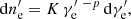
where Rj is the jet radius, hj is the specific enthalpy, and vj is the jet velocity. The specific enthalpy is calculated as in Choi & Wiita (2010),
![Mathematical equation: $$ \begin{aligned} h&= \dfrac{5c^2}{2\xi } + \left(2 - \kappa \right) c^2 \left[ \dfrac{9}{16}\dfrac{1}{\xi ^2} + \dfrac{1}{\left(2 - \kappa + \kappa \mu \right)^2}\right]^{1/2}, \\ &+ \kappa c^2 \left[\dfrac{9}{16} \dfrac{1}{\xi ^2} + \dfrac{\mu ^2}{\left(2 - \kappa + \kappa \mu \right)^2}\right]^{1/2} \end{aligned} $$](/articles/aa/full_html/2025/01/aa51914-24/aa51914-24-eq3.gif) (2)
(2)
with ξ = ρc2/p (p being the gas pressure), κ = np/ne being the ratio of proton and electron number density, and μ = mp/me.
For the particular configuration of the magnetic field used, the transversal equilibrium at injection leads to
 (3)
(3)
where pj, 0, pa, 0, and  are the mean jet pressure, the ambient pressure, and the jet axial magnetic field at injection, respectively. The fact that this pressure is independent of the toroidal magnetic field is a consequence of the particular profile of the toroidal magnetic field used, as discussed in Martí (2015). As described in the following section, all the parameters defining the jet and ambient medium for the base model used in this work correspond to model J4_C of Anglés-Castillo et al. (2021).
The simulation box extends over a uniform grid described in cylindrical coordinates, r and z, respectively, over 20 pc and 2000 pc with an initial jet radius of Rj = 1 pc. The number of computational cells in each direction of the grid is set to 1600 × 10 000 and the axisymmetry of the problem imposes reflection at r = 0. As the mass-loading scenario shows promising results for FR I jets, the total power injected into the jet is set to Lj = 1043 erg · s−1. At the injection, the jet is purely leptonic with a fraction Xe = ρe/ρ = 1.0, where ρe and ρ are the leptonic and full rest-mass densities, respectively. As the jet propagates, the composition is set to evolve through mass loading of the star. Table 2 sums up the parameters used at the injection point (labeled with subscript 0), either in the ambient medium or in the jet (respectively labeled a and j). From those parameters, one can derive the mean gas pressure in the jet pj, 0, the axial field  and toroidal field Bj, 0ϕ(r), and the maximum toroidal field Bm, j, 0ϕ. Such derivations can be seen in Anglés-Castillo et al. (2021), and full details of the parameters can be seen on their Table 1. We select the model labeled J4_C as our fiducial model, which corresponds to an average case of a jet with a significant amount of kinetic energy flux (Fk ∼ 28%; see their Table 2).
Jet, ambient medium, and stellar wind parameters used in the simulations, based on the J4_C jet set up shown in Anglés-Castillo et al. (2021).
2.2. Ambient medium and mass load
We consider an ambient medium pressure profile as described in Anglés-Castillo et al. (2021) (see also Perucho et al. 2014), namely a power law that reproduces a typical galactic atmosphere with
 (4)
(4)
where rc represents the inner core radius, and α = −1.095. Table 2 shows the mass-loading rate of ionized hydrogen (proton–electron) at the jet base, Q0. Along the jet propagation axis, the average mass-loading rate follows the profile
 (5)
(5)
where rc, s is the stellar core radius; as in Anglés-Castillo et al. (2021), we set αs = −1.095. Here, we make the assumption that the mass-loading profile follows the stellar distribution profile. This is motivated by the fact that mass loading should be driven by jet–star interactions, either from direct mass loading from stellar winds, and/or by mass entrainment from the ambient medium due to the development of small-scale instabilities at the jet boundary triggered by stars entering and leaving the jet (Perucho 2020). Moreover, from both analytic estimates and numerical simulations, it is known that stars can cross the jet without direct interaction, as the equilibrium point between the stellar wind and the jet flow is far beyond the star surface (Komissarov 1994; Bosch-Ramon et al. 2012; Perucho et al. 2017). The total number of stars in a jet within its initial 10 kpc is expected to be in the range of 108–109 (Wykes et al. 2014; Vieyro et al. 2017). Finally, the stellar distribution profile used here is valid for giant elliptical galaxies, which are the typical hosts of FR I/II jets.
2.3. Radiative transfer with the RIPTIDE code
We used the RIPTIDE code to compute synthetic synchrotron emission maps (Fichet de Clairfontaine et al. 2021, 2022). We first consider a population of nonthermal electrons with the associated number density described by the power-law distribution
 (6)
(6)
where K is the normalization constant of the power law with spectral index p = 2.2 – which is a typical value for mildly relativistic shock acceleration (Ostrowski & Bednarz 2002; Lemoine & Pelletier 2003) –, extending between γ′e, min and γ′e, max.
The normalization constant and the minimum electron Lorentz factor can be derived as described in Gómez et al. (1995):
 (7)
(7)
 (8)
(8)
where n′e is the number density of the nonthermal electrons, and e′e its corresponding energy density. Finally, CE = γ′e, max/γ′e, min = 103, which is constant, as we are neglecting radiative losses. This last assumption is supported by the fact that at 1 kpc from the jet base, considering typical values of γ′e, max = 105 and B′ = 1 mG, the synchrotron radiative cooling timescale remains longer than the adiabatic one, with cooling lengths of several kiloparsecs, which is longer than the simulated jet. In the previous expression, both parameters n′e and e′e are retrieved from the numerical simulations, assuming that they are proportional to the leptonic number density and the leptonic internal energy density, respectively (Böttcher & Dermer 2010; Mimica & Aloy 2012; Fromm et al. 2016). In this work, the respective proportionality constants are set to ξe = 0.1 and ϵe = 0.1 following previous procedures (Gómez et al. 1995; Mimica & Aloy 2012; Fromm et al. 2016; Fichet de Clairfontaine et al. 2021).
Accepting that our model is phenomenological, our approach is based on simple assumptions about the electron nonthermal population, leaving aside the details of the acceleration mechanisms responsible for the transfer of internal energy from the jet flow. Beyond this limitation, in the adopted model, γ′e, min is proportional to e′e/n′e, which is the (average) energy per (nonthermal) particle, which is reasonable. Additionally, this energy per (nonthermal) particle is proportional on its own to the internal energy per fluid particle. Furthermore, the fact that we fix the ratio between the maximum and minimum Lorentz factors of the power-law distribution, CE, also seems plausible given the properties of the jets at the studied scales. Once this simple model was chosen, the welcome result is that, in many instances, γ′e, min (and the whole particle distribution) shifts to larger values downstream from the jet (due to the dissipation of kinetic energy), which is on the basis of the positive radio-optical offsets obtained in the present work.
The synchrotron emissivity jν′ and absorption αν′ coefficients are computed in the jet frame according to the approximations shown in Katarzyński et al. (2001). Transformation into the observer frame is accounted for through the following relations (Rybicki & Lightman 1979):
 (9)
(9)
 (10)
(10)
These relations, which are valid for a steady jet flow, depend on the Doppler factor δ = (γj(1−βj⋅cos(θobs)))−1, with βj = vj/c and θobs being the angle between the direction of the jet axis and the line of sight. Now, the resulting specific intensity at a given cell with index i along a line of sight for an observer in the absolute frame is
 (11)
(11)
where Iν, i − 1 is the incident intensity on the cell i, τν, i is the optical depth due to synchrotron self-absorption and Sν, i = jν, i/αν, i is the synchrotron source function, which is considered constant inside the cell. For each line of sight, the emergent specific intensity is then Iν = Iν, N, with N being the total number of jet cells crossed by the line of sight. The incident specific intensity entering the jet is set to Iν, 0 = 0.
The computed synchrotron intensity Iν is converted into a synchrotron flux Fν:
 (12)
(12)
with Se being the emitting surface and DL the luminosity distance that depends on the shift of the source z. We neglect the impact of the light-travel-time delays, as we are interested in the steady state of the source (e.g., Fichet de Clairfontaine et al. 2022).
We apply an optical flux selection criterion based on the sensitivity of the Gaia mission to the integrated optical flux, as computed from our RIPTIDE model. Specifically, in the AB magnitude system, the Gaia telescope has a flux sensitivity of FAB,Gaia = 10−4 Jy at a 3σ confidence level according to the DR3 catalog (Gaia Collaboration 2021). This means that only sources with an optical flux above this threshold are considered for analysis. Similarly, we apply a radio flux threshold at the milli-Jansky (mJy) level. However, this radio flux cut does not significantly affect our results, as the optical flux selection is more restrictive and is thus the primary factor that determines which sources are included in our study. For our continuous radio and optical emission maps, we define the coordinates in terms of the centroid position (maximum flux position) of the emission, and we build the angle between the radio and the optical peak, denoted as Ψ (as in P19).
3. Radio–optical positive offsets
3.1. Energy dissipation
At the scale relevant to this study, jets are accelerated and we expect that magnetic acceleration has already taken place (e.g., Ricci et al. 2024). Thus, the jet must carry a non-negligible amount of kinetic and internal energy. Here, we chose the simulation labeled J4_C from Anglés-Castillo et al. (2021) as it represents a mildly kinetic jet and is positioned between the two cases studied in their paper: a kinetically dominated jet (J4_A) and an internal-energy-dominated jet (J8_X). Our choice of J4_C allows the exploration of an intermediate scenario. Additionally, we tested the energy dissipation behavior across these three cases and verified that while the J8_X configuration shows no energy dissipation, both J4_C and J4_A exhibit similar levels of energy dissipation due to their kinetic properties, which is consistent with Anglés-Castillo et al. (2021). This also aligns with the conclusions of Bowman et al. (1996) and the findings in Anglés-Castillo et al. (2021), which highlight that energy dissipation occurs primarily in kinetically-dominated jets due to mass-loading processes, increasing internal energy.
To study the presence and characteristics of radio-optical offsets, we first investigated the impact of different stellar distributions by setting rc,s = 1.0 kpc and 1.5 kpc. Figure 1 shows 2D maps of the nonthermal electron number density n′e (left) and the nonthermal electron energy density e′e (right) for an average mass-loading rate of Q0 = 5 × 10²³ g · yr−1 · pc−3. For such a low Q0 value, the jet still appears collimated (θopen ∼ 0°), while a local increase in the nonthermal energy density can be seen due to mass loading (with a maximum value at an axial distances of Z ∼ 0.9 kpc and Z ∼ 1.2 kpc, respectively), which is related to the value of rc, s. Due to the incorporation of protons, the ratio of the number of protons per electron κ increases with Z.
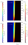 |
Fig. 1. Jet simulations with Q0 = 5 × 1024 g · yr−1 · pc−3, the nonthermal electron density (left), and their associated nonthermal energy density (right) for the two stellar distributions rc,s= 1.0 kpc (top) and rc,s= 1.5 kpc (bottom). Axes are given in parsecs. |
The ambient medium can also play a role in the radiative jet profile, allowing jet expansion within steep pressure profiles, or the opposite. To investigate the dependence of n′e and e′e on the ambient gas density and stellar distributions, we computed the electron number density n′e and the associated nonthermal energy density e′e profiles for various values of rc and rc, s. Figure 2 shows various profiles of those variables for different sets of rc and rc, s for a fixed value of Q0 = 5 × 10²³ g · yr−1 · pc−3. As shown, the position of maximum energy dissipation (maximum of the nonthermal energy density) evolves according to the value of the core radii. In parallel, the electron number density decreases at different rates. We suggest that a positive radio–optical offset is likely to occur when the position of the maximum energy dissipation is away from the jet base because of the evolution of γe, min along the jet axis. Indeed, this displacement can be attributed to the fact that, as energy dissipation peaks further away from the jet base, the resulting emission at different wavelengths becomes spatially separated: both optical and radio emission would be localized along the jet axis, although at different axial positions.
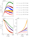 |
Fig. 2. Axial distance dependence of the nonthermal electron energy density e′e, density n′e, and minimum Lorentz factor γ′e, min evaluated along the jet inner axis, given in parsecs. In all cases, an average mass-loading rate of Q0 = 5 × 10²³ g · yr−1 · pc−3 was used. |
To study the presence and characteristics of radio–optical offsets, we produced synthetic images computed using RIPTIDE on the jet simulations. Unless stated otherwise, we construct emission maps for two frequencies in the observer’s frame νobs = 4.3 × 10¹⁰/5 × 1014 Hz (corresponding to typical VLBI/optical frequency) and for a given pair of jet viewing angle θobs and shift z, and thus evaluated in the jet frame. The axis of the emission maps is given in milliarcseconds for comparison with observations (P19). For reference, Figure 3 shows emission maps associated with the simulations shown in Figure 1, with a radio emission map shown on the left and the optical one on the right. Optical emission maps display a dimmer jet at the base, which becomes brighter with distance due to the increase in γ′e, min triggered by mass loading. A clear radio–optical positive offset dapp is seen in both cases, with values (∼0.4 and ∼ 1 mas, respectively) depending on the choice of the stellar distribution (rc, s).
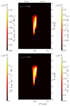 |
Fig. 3. Synthetic synchrotron flux maps in the radio (ν = 3 × 10¹¹ Hz, left) and in the optical band (ν = 5 × 10¹⁴ Hz, right) from simulations shown in Figure 1. We display the results for the two stellar distributions rc,s = 1.0 kpc (up) and rc,s= 1.5 kpc (down) for a viewing angle θobs = 10°, a redshift z = 1.4, a fixed |

To study the radio–optical positional offsets, dapp, for a range of Ṁ values, we measured the offset values for a set of emission maps by fixing the jet observation angle, θobs = 5°, and redshift, z = 1. These values are the medians derived by the authors from the collection of quasars in P19.
Figure 4 shows the variation of dapp with Ṁ for the same set of core radii rc and rc, s. The radio–optical offset decreases with increasing values of the mass-loading rate. For low Ṁ, not only does the energy dissipation occur at a lower rate but also the optical emission peak appears at a larger distance from the jet base. This configuration thus results in higher values of the radio–optical offset, as dissipation takes place in an extended region, as opposed to strong mass loading, in which deceleration is fast and therefore dissipation takes place at the jet base. Therefore, the tendency for dapp separation to decrease with Ṁ is mainly due to the increase in the mass load in the jet per unit of distance.
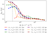 |
Fig. 4. Dependence of the apparent radio–optical offset dapp on the average mass load Q0 for various ambient medium and stellar core radii (rc and rc, s). Offsets on the right side of the vertical black dashed lines represent minimum offsets detectable by Gaia according to our selection criteria. |
Consequently, the location of maximum energy dissipation begins to drift closer toward the jet base, causing the radio and optical centroid emissions to converge closer to the origin. At high Ṁ values, this convergence intensifies, and the radio-optical emission offset approaches zero, indicating a minimal spatial separation between these emissions close to the jet base. As a competing effect, the optical flux increases with increasing values of Ṁ, making the jet detectable by Gaia. The vertical dashed line represents, in that case, the lowest Ṁ value that allows detection by Gaia. Therefore, one needs a proper range of Ṁ that allows a sufficiently high optical flux for detection and also extended dissipation. Overall, our results suggest the existence of an ideal average mass-loading range, allowing us to observe a detectable and non-zero radio–optical offset spanning from 5 × 10²³ to 5 × 1024 g · yr−1 · pc−3.
Regarding the role of the gas and stellar distributions of the host galaxy, we observe that increasing rc, s generally results in larger values of dapp, indicating that the peak energy dissipation occurs further from the jet base. Conversely, smaller values of rc favor fast jet expansion, causing the capture of more stars inside the jet and favoring jet deceleration, which in turn causes the peak energy dissipation to move closer to the jet base. It appears that the larger the galaxy, the greater the radio–optical offset value, putting aside observational biases regarding the viewing angle and redshift.
3.2. Distribution of radio–optical offsets
Interestingly, from all our simulated cases, we find a typical offset value close to the median one found by P19, with dapp ∼ 0.7 mas, and typical quasar parameters of θobs = 5° and z = 1 (see Figure 4). However, the reliability of this result should be taken with caution, since our analysis considers all the jets that are detectable, without accounting for the angular-resolution limits of Gaia. To extend this study to a larger range of observation angles and redshift, and simulate observations of jets, we randomize a set of 1000 sources with a uniform distribution of observation angles from 1° to 30°, and a uniform distribution of different redshifts from 0.5 and 2. The choice of uniform distributions is solely based on avoiding the introduction of additional bias.
For each set of sources, we used eight values of Q0 ranging from 5 × 10²³ to 5 × 1024 g · yr−1 · pc−3. Additionally, we tested the two cases of different stellar distributions, rc,s = (1.0,1.5) kpc, for a common ambient medium (rc = 1.0 kpc), which allows us to study the impact of the stellar distribution in isolation, a choice based on the findings shown in Figure 4. The results are shown in Figure 5, where the left column represents the distributions of the angles between the optical and radio peak directions Ψ2 as measured from the jet base (see Sect. 1) and the right column shows the distributions of offsets dapp for different average mass-loading rates and stellar core sizes. We limit the results shown to the cases for which the optical emission can be detected by Gaia according to its sensitivity. Although we consider a straight (linear) jet here, one could simulate bent jets to study how the peak positions of the optical emission evolve in response to Doppler boosting, which may also cause a small, non-zero Ψ. Taking into account the limited angular resolution of Gaia will reduce the presence of non-zero Ψ values.
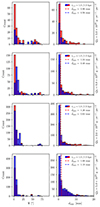 |
Fig. 5. Histograms of the radio–optical angle (Ψ, left) and apparent offset (dapp, right) for the set of randomized synthetic emission maps. Each row represents histograms for a given average mass-loading Q0 and for a given star distribution (rc,s= 1.0 kpc in blue and rc,s = 1.5 kpc in red; dark blue represents the overlap). Vertical dashed lines in the panels of the right column represent the associated median radio–optical offset. |
In all cases, positive offsets are obtained with dapp ≳ 0 mas and Ψ ∼ 0°. A stellar distribution with rc,s = 1.0 kpc leads to smaller median offsets, dapp (as seen in the histograms of Figure 5), as already discussed.
Figure 6 presents the dependency of the offset values dapp for jet cases detectable by Gaia – extracted from our dataset of 1000 synthetic jet emission maps – on redshift z (left column) and viewing angle θobs (right column). Each plot includes solid lines that illustrate the average radio–optical offset for different mass-loading profiles in each redshift (0.1) or viewing angle (1.0°) bin, as detailed in the legend; we also show the angular resolution provided by Gaia. The top and bottom rows of each column correspond to star distributions with core radii rc, s of 1.0 kpc and 1.5 kpc, respectively. This layout highlights the effects of observational biases, such as those related to redshift and observation angle, on the apparent displacement for a constant mass-loading value.
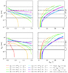 |
Fig. 6. Dependence of the apparent radio–optical offset dapp on the redshift z (left column) and jet observation angle θobs (right column). For various average mass-loading rates Q0 (see legend), solid lines represent the average across our randomized set of jets. Results are displayed for the two stellar distributions tested (rc,s = 1.0 kpc first row and rc,s = 1.5 kpc second row), with a fixed gas distribution of r_{\mathrm{c}} = 1.0 kpc. The horizontal black lines illustrate the medians dapp obtained by P19 for quasars (0.7 mas, dashed line), radio galaxies (2.3 mas, dash dotted line), and Seyfert 2 (7.2 mas, dotted line) in the case of significant offset detection. We also show the typical Gaia angular resolution as a solid black line for qualitative comparisons. |
Indeed, due to the selection effect imposed by the sensitivity of Gaia, a larger radio–optical offset will be detectable for low-redshift sources and large observation angles. The physical impact of the mass-loading profile can be seen by the great differences between 5 × 10²³ and 5 × 1024 g · yr−1 · pc−3, where the offset dapp can vary by a factor 10 (for a constant redshift, or a constant observation angle). For large mass-loading values, the average profiles of dapp seem to converge as the effect of mass loading saturates. Assuming the mass loading is mainly driven by stellar winds, we can relate the detectability of the flux of the jets by Gaia to the distribution of stars in the host galaxy. Jets that experience lower mass loading are more likely to be detected for larger stellar core radii, as more stars interact with the jet. For example, a jet encountering an average mass load of approximately Q0 = 5 × 1024 g · yr−1 · pc−3 is detectable when the core radius of the star distribution, rc, s, is about 1.5 kpc, but not at 1.0 kpc. In general, increasing the core radius, rc, s, leads to a larger apparent distance, dapp, and a greater optical flux for a given average mass-loading rate, Q0.
On Figure 6, we also highlight median offsets for quasars, dapp = 0.7 mas, radio galaxies, 2.3 mas, and Seyfert 2 galaxies, 7.2 mas, which is in remarkable agreement with the observational values given by P19 from their sample. These median values are particularly interesting, as they underline the dependence of the radio–optical offset on the Doppler effect. Indeed, from our results, quasar objects can be observed at larger redshifts (between 1 and 1.5) and lower observation angles 0° to 10°, while radio galaxies should be observed at lower redshifts and larger observation angles, which is even more pronounced for Seyfert 2 galaxies. Those findings align perfectly with both P19 and our current knowledge on AGN classification (e.g., Netzer 2015).
Regarding the effects of the stellar distribution, we note that a decrease in the stellar core radius from rc,s = 1.5 kpc to rc,s = 1.0 kpc shifts the apparent radio–optical offset to smaller values (requiring an increase in the viewing angle by several degrees in order to recover the original apparent offset). A larger stellar core holds the dissipation of energy over longer distances, causing the peak energy dissipation to move away from the jet base. Assuming a range of average mass-loading profiles, the different jet profiles can exhibit varied deceleration characteristics, which influence the optimal observation angles for detecting similar displacement values. It is important to note that, as we do not impose any dependence of the average mass-loading rate on galaxy redshift, the differences in detectability and dapp values are primarily due to selection biases related to the observational setup.
3.3. Color magnitude of the jet
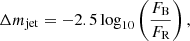
P19 show how the presence of a bluer object is generally linked to the presence of an accretion disk (and of a so-called big blue bump component), which translates into a negative radio–optical offset. Indeed, in those cases, the optical centroid is shifted towards the base of the jet. Therefore, redder objects seem to be linked to objects showing positive radio–optical offsets and a relatively weak accretion disk component. Although the inclusion of an accretion disk component is beyond the scope of the present paper, one can estimate the magnitude difference Δmjet between the blue and red bands of the Gaia telescope in the jet. This parameter is estimated as
 (13)
(13)
where FR and FB are respectively the fluxes as measured in the red and blue bands of Gaia. For simplicity, we consider the wavelength centered in the middle of each band, respectively, at R ∼ 850 nm and B ∼ 550 nm (Jordi et al. 2010). Consequently, a larger positive value of Δmjet indicates a redder jet.
Figure 7 shows the variation of Δmjet as a function of the average mass-loading rate for the two-star core radii rc,s = 1.0 kpc and 1.5 kpc. The results for the two stellar core radii are almost indistinguishable, with red fluxes dominating over blue fluxes. In both cases, the red excess tends toward a minimum increasing Q0, as larger mass-loading rates increase the amount of dissipated energy and therefore the optical flux.
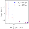 |
Fig. 7. Dependence of the average magnitude difference Δmjet between blue (B) and red (R) bands with the mass-loading rate Q0. Results are displayed for the two stellar distributions tested, rc,s = 1.0 kpc in blue, and 1.5 kpc in red, with associated 1σ standard deviation uncertainty bars as we average over the θobs and z distribution. |
Smaller Q0 values lead to larger radio–optical offsets, and are correlated with redder magnitude, as observed and discussed in P19. Putting aside the accretion disk contribution to the overall magnitude, our results show that redder objects should imply lower mass-loading rates, and observable (discernible) positive radio–optical offsets according to our results. For larger values of Q0, the difference in color magnitude saturates as the increase in Q0 causes dapp to converge to zero.
Petrov & Kovalev (2017a) underline that the optical centroid detected by Gaia is dominated by compact, jet-related emission rather than by diffuse stellar light from the host galaxy. However, if a significant part of the mass loading in the jet originates from stellar winds, the presence of a stellar population could impact the radio–optical offset and potentially alter the magnitude estimates in our analysis. As the optical emission of the jet is highly compact compared to the extended stellar distribution, the impact of the stellar luminosity on the optical centroid position is expected to be limited. A detailed inclusion of this component falls outside the scope of this paper, but future work could include a consideration of specific stellar types and distributions, as the influence on Gaia’s optical centroid may vary in galaxies with substantial mass loading from stellar sources. Still, our results are consistent with the observational results of P19, although we cannot compare the magnitude difference calculated in the present study with the Gaia color observed because of both physical (the accretion disk and stellar population are not simulated here) and instrumental aspects.
4. Discussion
4.1. The mass-loading scenario
We used RMHD numerical simulations of jets including source terms that account for mass loading, following previous work by Anglés-Castillo et al. (2021). With these simulations, we studied the possible role of dissipation in the presence of radio–optical offsets by means of the radiative transfer code RIPTIDE. We have chosen a fixed jet power of Lj = 1043 erg · s−1 – a typical value for FR I jets (Perucho 2020) –, for which the proposed scenario shows promising results. Our choice of approach is based on the fact that efficient dissipation is known to largely coincide with the region in which jet deceleration takes place (see Figure 1), as shown by Laing & Bridle (2014). Due to the conversion of kinetic energy into internal energy, the minimal Lorentz factor of the nonthermal electrons increases with distance according to their nonthermal energy density (see Figure 2). The presence of nonthermal emission from a population of accelerated particles is suggested from optical polarimetry observations (Kovalev et al. 2020), and we indeed derive positive radio–optical offsets from our synchrotron maps. Jet–star interactions are unavoidable in the jets (Wykes et al. 2014; Vieyro et al. 2017), and they may play a relevant role in jet deceleration according to several theoretical (e.g., Komissarov 1994; Perucho 2020) and observational works (Mingo et al. 2019). Although the setup differs, our radio emission maps bear similarities to those observed in Mimica et al. (2009), particularly in the case of stationary, pressure-matched jets relative to the ambient medium. Despite not accounting for radiative losses due to their specific parameters, these latter authors demonstrate that such losses shorten the emission morphology, while the centroid remains in the same position. Nevertheless, at the scale studied here, we consider that the leading cooling process is driven by adiabatic expansion. It should be noted that jet bends or other dissipation processes such as shocks or turbulence could imply an additional shift of the radio–optical centroid beyond those analyzed here based on the jet mass loading.
As our model to explain radio–optical offsets is based on the dissipation of kinetic energy, we have chosen one of the models analyzed in Anglés-Castillo et al. (2021) with a large fraction of kinetic flux as the base jet model of our study. At the scales relevant to this study, jets appear to be relativistic and tend to carry a significant amount of kinetic energy, which is consistent with theoretical and numerical findings. Among them, our results align with the condition set in Perucho (2019) (see equation (27)). In addition, these findings indicate that beyond the acceleration region, typically a few parsecs from the jet base, jets are predominantly kinetically dominated (Vlahakis & Königl 2004; Komissarov et al. 2009; Komissarov 2012; Ricci et al. 2024). This aligns with the dissipation mechanisms required to produce the observed radio–optical offsets. Here we show that, for a certain regime of average mass-loading rates, ranging from 5 × 10²³ to 5 × 1024 g · yr−1 · pc−3, the dissipation produced in the jet may result in radio-to-optical peak offset values of between dapp ≃ 0.4 mas and 10 mas, which is consistent with observations of different types of AGN (see Figure 4 for application to quasars). Indeed, jets at large redshifts and small observation angles are consistent with the quasar population. In contrast, smaller redshifts and larger observation angles are consistent with radio galaxies and Seyfert types (P19). In this sense, the impact of Doppler boosting appears crucial to our understanding of the characteristics of radio-optical offsets (Secrest 2022).
Our results indicate the presence of a higher average mass-loading rate for radio galaxies and Seyfert 2 galaxies. The latter type is known to host star-forming regions, which could locally enhance the average stellar mass-loss rate (Rodriguez Espinosa et al. 1987), potentially affecting the radio–optical offset. Our color magnitude estimation indicates that detectable offsets are correlated with relatively red objects (see Figure 7), which is also consistent with observations (P19; Lambert et al. 2024). Although we did not model the emission from the stellar population, its contribution into the optical centroid, and therefore on the radio–optical offset, should be limited (Petrov & Kovalev 2017a). Nevertheless, our color–magnitude estimate cannot be compared directly to observations, as we did not account for instrumental effects.
Our results implicitly predict a non-negligible gamma-ray (and very high-energy gamma-ray) emission from jet–star interactions. Indeed, jet–star interactions are often listed to explain multiwavelength, and especially gamma-ray, emission in jetted AGN (Barkov et al. 2010; Bosch-Ramon et al. 2012; de la Cita et al. 2016; Vieyro et al. 2017; Torres-Albà & Bosch-Ramon 2019). This could at least partly explain, for example, the extended emission detected from Centaurus A in the tera-electronvolt (TeV) band (H. E. S. S. Collaboration 2020), where the mass-loading scenario has been invoked to explain its broadband emission and the production of very energetic cosmic rays (Wykes et al. 2013, 2014). Accounting in the future for radiative cooling (if relevant) and the presence of other dissipative processes (such as mass entrainment at the jet boundaries) will refine our results, and will clarify the role of jet–star interactions in more complex jets.
4.2. Implications on the jet power
We fixed the jet power at Lj = 1043 erg · s−1, a typical value for FR I jets (e.g., Perucho 2020). However, jet power typically ranges from Lj = 1042 erg · s−1 to Lj ≤ 1048 erg · s−1 (Ghisellini & Celotti 2001). High jet power reduces the effects of mass entrainment and energy dissipation due to mass loading (Perucho et al. 2014), probably bringing the offset to zero or negative values. Conversely, lower jet power efficiently dissipates energy along the deceleration region, which could explain the radio–optical offsets observed. For jets with powers higher than our initial value, detectable radio–optical offsets should persist down to the optical detection limit and turn out null or negative due to the lack of energy dissipation. Lower jet power should also result in reduced offsets, converging to zero, due to intense energy dissipation.
In summary, in our framework, there are three power regimes: (1) jets with the lowest powers would be decelerated close to the forming region, thus dissipating most of their kinetic energy, and this would result in zero or undetectable offsets; (2) the regime studied here would show positive offsets for the expected stellar populations in their host galaxies, and (3) high-powered jets undergo little dissipation within their host galaxies, as shown by their bulk velocities at kiloparsec scales, which means that they would tend to have zero or negative offsets, as expected from the conical jet-expansion models (Blandford & Königl 1979; Marscher & Gear 1985).
However, the above statements leave us to question why Plavin et al. (2019) observe such a fraction of positive offsets. The answer should be related to the jet-power distribution, as well as the stellar populations interacting with the jet. Jets of sufficiently low power (< 1042 erg · s−1) will not show extended emission, as they must be decelerated inside the host galaxy. Therefore, the fraction of positive offsets observed suggests a distribution of jet power peaking around 1043 erg · s−1. The presence of positive radio–optical shift, as explained in our model, will lead to low-power jets interacting with mainly main sequence stars with weak stellar winds within their first kiloparsecs (similar to the case studied here), and high-power jets with a lower density of red-giant stars. This aspect is explored in more detail in the following section.
4.3. Implications on the mass-loading origin
All jets must entrain some amount of stellar matter, which may or may not significantly decelerate the jet depending on the jet power and stellar populations (Hubbard & Blackman 2006; Perucho et al. 2014; Anglés-Castillo et al. 2021). If we assume that the mass entrained by the jet is only that driven by stellar winds, then the average mass-loading necessary to account for the observed radio–optical offsets translates into an average stellar mass-loss rate per unit volume ranging from 10−10 to 10−9 M⊙ · yr−1 pc−3.
While K-M type stars are the most abundant in giant elliptical galaxies (van Dokkum & Conroy 2010), they have low mass-loss rates (< 10−12 M⊙ · yr−1), implying unrealistically large stellar densities to account for the needed mass loads. However, in the case of red giants, whose wind losses span from 10−10 to 10−5 M⊙ · yr−1 (Reimers 1975), number densities of 10−3 − 1 star per cubic parsec should be sufficient to account for the observed radio–optical offsets. The density of red giants depends on the star formation history, and on the age of the galaxy. As jet-hosting galaxies have typically low star-formation rates and host old populations of stars (Zhu et al. 2010; Heckman & Best 2014), it is likely that red giants are relatively abundant and that their density is within the range mentioned above. It is worth mentioning that jet–red-giant interactions have already been studied in the past to explain several aspects of jet physics and its potential impact on the nonthermal emission of jets (Barkov et al. 2010; Bosch-Ramon et al. 2012; Khangulyan et al. 2013; Perucho et al. 2017).
Our results suggest that misaligned jets, such as those in radio galaxies and particularly Seyfert galaxies, should show a higher mass-loading rate than those associated with quasars on average, for fixed jet power, that is, to explain the observed offsets. In the case where stellar wind dominates mass loading, this would require the presence of star-forming regions, and different stellar populations with a larger fraction of very luminous stars that exhibits very high stellar wind loss, as we discuss below.
However, even if we assume that the main source of dissipation is the interaction with stars, distinguishing between different average stellar mass-loss rates can be challenging due to overlapping effects, particularly at lower dapp values. This overlap introduces a degeneracy that is not only dependent on rc, s, the stellar core radius, but also on other factors, such as the ambient gas and the jet properties. The observed degeneracy occurs because different combinations of mass-loading values and core radii can produce similar dapp outcomes. This is especially the case when only considering one observational parameter: for example, a larger gas core radius might mimic the effects of a higher mass-loading rate in terms of reducing dapp.
The impacts of other jet parameters and the power-law indices for ambient gas and stellar distributions on the radio-optical offset are complex and are beyond the scope of this paper. However, one possible approach to addressing the rc, s degeneracy is to analyze the average ratio between the radio and optical fluxes (estimated at 4.3 × 10¹⁰ Hz and ν = 5 × 10¹⁴ Hz, respectively) for all selected sources at a given average mass-loading value Q0. By averaging the flux ratio over many sources, the specific geometric conditions of individual sources tend to cancel out. The results are displayed in Figure 8. The figure shows that the differences in flux ratio between the two stellar core radii are limited, but could allow us – through observational data – to distinguish the profile of mass loading. If the shift is mainly caused by stellar winds, this analysis would be feasible only for measured, positive radio–optical offsets. For instance, knowing z, the stellar mass-loss rates per unit volume (by characterizing the stellar populations and densities in galaxies) and rc, s might help to constrain θobs. Alternatively, using independent measures of the viewing angle and rc, s, one could constrain the population and distribution of stars in the core of galaxies.
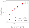 |
Fig. 8. Dependence of the average optical/radio flux, Foptic/Fradio (as measured at ν = 3 × 10¹⁰ Hz and ν = 5 × 10¹⁴ Hz, respectively) on the average mass-loading rate Q0. Results are displayed for the two stellar distributions tested, rc,s = 1.0 kpc in blue, and 1.5 kpc in red with associated 1σ standard deviation uncertainty bars as we average over the θobs and z distribution. |
In high-power jets, the fraction of energy dissipated is much smaller and, although an increased average stellar mass-loss rate could result in observable radio-optical offsets (see Figure 4), the values necessary to produce observed positive offsets are probably too large to be realistic. Therefore, the offsets are expected to be visible mainly in the case of low-power jets. In this case, we could expect observable offsets to emerge for more realistic average stellar mass-loss rates (see Figure 2). However, in all cases, a non-uniform stellar distribution, where densities vary significantly across the galactic atmosphere (Gebhardt & Thomas 2009; Vieyro et al. 2017), must be considered for quantitative comparisons with observations.
From a broader perspective, a more plausible hypothesis might be that mass loading could be driven not only by stellar wind but also by mass entrainment. For instance, Matsumoto et al. (2017), Gourgouliatos & Komissarov (2018), Perucho (2020) discussed how small-scale instabilities or the penetration of stars into the jet can initiate mixing layers, leading to mass loading and jet deceleration. This weakens the capacity of our model, to constrain the stellar population.
4.4. Observational biases
Doppler boosting has a crucial impact on the detection of radio–optical offsets. We have shown that the sources showing an offset of close to zero are over-represented in the set selected according to Gaia sensitivity (see Figure 5), which is in agreement with Petrov & Kovalev (2017b), Petrov et al. (2019). This is mainly due to the contribution of jets with small viewing angles, for which the emission is Doppler boosted. In that case, the majority of the sources are detected in the optical band regardless of the average stellar mass-loss rate (see Figure 6, right).
The influence of cosmological distance on the detection is most evident in the case of low average mass loading (Q0 ≤ 5 × 10²³ g · yr−1 · pc−3), where low-redshift sources can be over-represented (see Figure 6, left). This effect is weaker in the case of medium to high average mass-loading rates (Q0 > 5 × 10²³ g · yr−1 · pc−3), because the strong dissipation makes them brighter and therefore detectable at larger distances. Thus, the recent and future improvements in Gaia’s sensitivity, which has been enhanced through continuous advancements in its instruments and data-processing techniques (Gaia Collaboration 2021), are crucial to leveraging the impact of observational biases to fully test our predictions with observations.
Finally, observational results from Secrest (2022) indicate that the prevalence of radio–optical offsets tends to decrease with increasing optical variability, which could be the consequence of the small line-of-sight angles typical of highly variable sources. This result will be investigated in a follow-up study.
4.5. Predictions from the mass-loading scenario
The mass-loading scenario presented in this paper may provide not only predictions of measurable observables, such as radio–optical offsets and color magnitudes, but also constraints on the jet power, a parameter notoriously difficult to deduce from observations (Hardcastle 2018; Perucho 2019). Jet power is typically inferred from secondary indicators, such as luminosity (Daly et al. 2012; Godfrey & Shabala 2013) and emission line features, which can be affected by multiple factors, including Doppler boosting, viewing angle, and interaction with the ambient medium (Ghisellini & Celotti 2001; Fujita et al. 2016; Foschini et al. 2024).
Our results demonstrate that there is a plausible, independent way to estimate jet power in cases where radio–optical offsets are detected, which we explain here. For a given jet host galaxy with a known redshift z, optical observations can provide an estimate of the stellar distribution rc, s, the color index, or the radio-to-optical flux ratio (see Figure 8), and together with radio observations, the radio–optical offset.
The jet parameters that determine the observed radio–optical offset are the viewing angle θobs and the jet power Lj. If the former can be estimated from, for example, the jet-to-counter-jet flux ratio, our model can provide an independent estimate of the jet power. To a lesser extent, depending on the fraction of mass loading driven by stellar winds, we could also derive information on the stellar types, and on the potential fraction of red giants needed to explain the observed radio–optical offset.
The jet power is determined by the kinetic, internal, and magnetic energy fluxes, and so for a given value of power, different configurations are possible. Therefore, once power is estimated, and following Anglés-Castillo et al. (2021), we could further constrain the jet physics by defining regions of the parameter space for rest mass density, pressure, velocity, field intensity, and so on. These different configurations can also influence the observed offset: in this study, we have used a case where the jet is carrying a significant amount of kinetic energy from Anglés-Castillo et al. (2021) as a base configuration, because these can efficiently dissipate energy and thus explain the observed offsets. A kinetically dominated jet does not appear to be necessary to explain the radio–optical offsets; a small amount of kinetic energy is dissipated. We verified that internal dominated jet cases lead to null or negative offsets, and these were excluded from this study according to our purposes. Comparisons of our predictions with observations will allow us to confirm whether or not radio–optical offsets provide a way to predict fundamental AGN properties (Petrov & Kovalev 2017a; Wang et al. 2022). Future work should include the direct application of this method to specific sources, incorporating a detailed source analysis and setup to feed multidimensional, dynamical simulations, which would allow us to test the power of this approach.
5. Conclusions
Jet–star interactions are crucial for understanding multiwavelength observations and the dynamics of jets, particularly in the context of FR I galaxies. The mass-loading scenario provides a promising framework for partly explaining the dynamics of kiloparsec-scale jets, especially when considering typical FR I jet power levels. In this study, we ran RMHD simulations of mass-loaded stationary jets and used the radiative transfer code RIPTIDE to generate multiwavelength synthetic synchrotron emission maps. Focusing on galaxy properties, we thoroughly examined the radio and optical emission maps and the color magnitude. Our key findings are summarized as follows:
-
Jet deceleration and energy dissipation: Jets with a power of Lj = 1043 erg · s−1 experience deceleration and convert kinetic energy into internal energy, accelerating particles in the jet. This dissipation leads to an increase in the minimal Lorentz factor γ′e, min of nonthermal electrons along the jet under the prescription chosen here. This behavior is observed in jets with a sufficient kinetic energy budget, which is expected at the beginning of the deceleration or dissipation region (Laing & Bridle 2014).
-
Radio–optical offsets: The increase in γ′e, min results in spatially separated radio and optical peak emission regions. The radio-dominated region is located closer to the jet base where γ′e, min is low, while the optical-dominated region is located downstream close to the position where dissipation occurs, causing a positive radio–optical offset.
-
Impact of galaxy properties: The distribution of gas and stars in the host galaxy significantly influences the observed offset. Gas distribution, represented by its core size, rc, impacts mainly the location of the radio-dominated region, while stellar distribution, represented by rc, s, changes the position where most of the dissipation occurs. There is a fine balance between these two parameters, which results either in an extension or a limitation of the radio–optical offset.
-
Useful observables: The radio-to-optical flux ratio and the color magnitude permit us to derive the average stellar mass-loss rate present in the jet. We conclude that lower flux ratios and higher optical emission from the jet are linked to lower average stellar mass-loss rates and result in a more significant (positive) radio–optical offset.
-
Observational biases: The viewing angle of the jet and redshift affect the observed radio–optical offsets. Offset detectability is also intimately linked to flux sensitivity, especially in the optical band. We expect that low redshift and small viewing angles are over-represented in any dataset.
-
Observational evidence: Our work aligns with collected evidence that energy dissipation, and therefore nonthermal emission, occurs in the first few kiloparsecs of the jet from is base (Laing & Bridle 2014), which is also supported by optical polarimetry (Kovalev et al. 2020). For a certain average mass-loading rate regime, we are able to reproduce the typical range of the radio–optical offset properties observed, and for different types of AGN jets according to their viewing angle. In the case where mass loading is mainly driven by stellar winds, our results point to a dominant population of red giants interacting with the jet, with a plausible range of number density in the galactic core. The trend between the color magnitude of our simulated jets and their radio–optical offset is consistent with observations,although we do not account for optical emission from a stellar population, as its impact should be limited.
-
Observational predictions: From this scenario, and our results, we can predict that radio–optical offsets should evolve as a function of jet power. Jets of relatively low power (Lj < 1043 erg · s−1) should display null or negative offsets, with a more stable optical emission. FRI jets of greater power (1043 erg · s−1 < Lj < 1044 erg · s−1) should display observable, positive offsets. FR II jets (Lj > 1044 erg · s−1) should display null or negative offsets as the jet evolves in a conical way. For a given jet power, increasing (decreasing) the average mass-loading rate should decrease (increase) the apparent radio–optical offset. If we only consider stellar winds, this could be explained by different types of stellar populations dominating the average mass-loss rates. Mass entrainment from jet–star interactions could also imply a significant amount of mass loading in the jet, and is known to influence jet behavior and nonthermal emission.
To a lesser extent, we predict the presence of an extended gamma-ray emission component caused by inverse Compton, and the production of very energetic cosmic rays (protons and neutrinos) from mass-loaded jets. Notably, in the case of jet–red-giant interactions, local jet–star interactions could produce high- and very high-energy gamma-ray emission (Torres-Albà & Bosch-Ramon 2019), together with high-energy cosmic rays as neutrinos (Wykes et al. 2014, 2018; Wang et al. 2022).
Future work will focus on the study of the interplay between jet power and the average mass-loading rate. This will incorporate more detailed observational constraints from optical astronomy (such as the angular resolution provided by Gaia). A dedicated application to specific sources will be presented, where we will fix a range of parameters, such as the radio–optical offset, based on observations. This may allow us to understand the origin of the mass-loading derived here, and could potentially provide an independent estimate of the jet power in those cases. It will also allow us to study the jet physics at a unique level, offering a new multiwavelength view of the AGN classification.
In the Eq. (1) and throughout the whole paper, we absorb a factor  in the definition of the magnetic field.
We note that our models are cylindrically symmetric; non-zero radio–optical angles Ψ are unreliable and are a measure of the limitations of the procedure we used to detect the optical emission maxima.
Acknowledgments
We thank the reviewer for the constructive comments that improved the quality of the present manuscript. We thank Andrei Lobanov for valuable comments on the manuscript. This work has been supported by the Spanish Ministry of Science through Grant PID2022-136828NB-C43, from the Generalitat Valenciana through grant CIPROM/2022/49, from the Astrophysics and High Energy Physics program supported by the Spanish Ministry of Science and Generalitat Valenciana with funding from European Union NextGenerationEU (PRTR-C17.I1) through grant ASFAE/2022/005. YYK was supported by the MuSES project, which has received funding from the European Research Council (ERC) under the European Union’s Horizon 2020 Research and Innovation Programme (grant agreement No 101142396).
References
- Anglés-Castillo, A., Perucho, M., Martí, J. M., & Laing, R. A. 2021, MNRAS, 500, 1512 [Google Scholar]
- Barkov, M. V., Aharonian, F. A., & Bosch-Ramon, V. 2010, ApJ, 724, 1517 [NASA ADS] [CrossRef] [Google Scholar]
- Bicknell, G. V. 1984, ApJ, 286, 68 [NASA ADS] [CrossRef] [Google Scholar]
- Bicknell, G. V. 1994, ApJ, 422, 542 [NASA ADS] [CrossRef] [Google Scholar]
- Blandford, R. D., & Königl, A. 1979, ApJ, 232, 34 [Google Scholar]
- Blandford, R., Meier, D., & Readhead, A. 2019, ARA&A, 57, 467 [NASA ADS] [CrossRef] [Google Scholar]
- Boccardi, B., Krichbaum, T. P., Ros, E., & Zensus, J. A. 2017, A&A Rev., 25, 4 [NASA ADS] [CrossRef] [Google Scholar]
- Bosch-Ramon, V., Perucho, M., & Barkov, M. V. 2012, A&A, 539, A69 [NASA ADS] [CrossRef] [EDP Sciences] [Google Scholar]
- Böttcher, M., & Dermer, C. D. 2010, ApJ, 711, 445 [CrossRef] [Google Scholar]
- Bowman, M., Leahy, J. P., & Komissarov, S. S. 1996, MNRAS, 279, 899 [NASA ADS] [CrossRef] [Google Scholar]
- Bridle, A. H., & Perley, R. A. 1984, ARA&A, 22, 319 [NASA ADS] [CrossRef] [Google Scholar]
- Choi, E., & Wiita, P. J. 2010, ApJS, 191, 113 [NASA ADS] [CrossRef] [Google Scholar]
- Daly, R. A., Sprinkle, T. B., O’Dea, C. P., Kharb, P., & Baum, S. A. 2012, MNRAS, 423, 2498 [NASA ADS] [CrossRef] [Google Scholar]
- de la Cita, V. M., Bosch-Ramon, V., Paredes-Fortuny, X., Khangulyan, D., & Perucho, M. 2016, A&A, 591, A15 [NASA ADS] [CrossRef] [EDP Sciences] [Google Scholar]
- Falle, S. A. E. G. 1991, MNRAS, 250, 581 [Google Scholar]
- Fanaroff, B. L., & Riley, J. M. 1974, MNRAS, 167, 31P [Google Scholar]
- Fichet de Clairfontaine, G., Meliani, Z., Zech, A., & Hervet, O. 2021, A&A, 647, A77 [NASA ADS] [CrossRef] [EDP Sciences] [Google Scholar]
- Fichet de Clairfontaine, G., Meliani, Z., & Zech, A. 2022, A&A, 661, A54 [NASA ADS] [CrossRef] [EDP Sciences] [Google Scholar]
- Foschini, L., Dalla Barba, B., Tornikoski, M., et al. 2024, Universe, 10 [Google Scholar]
- Fromm, C. M., Perucho, M., Mimica, P., & Ros, E. 2016, A&A, 588, A101 [NASA ADS] [CrossRef] [EDP Sciences] [Google Scholar]
- Fujita, Y., Kawakatu, N., & Shlosman, I. 2016, PASJ, 68, 26 [CrossRef] [Google Scholar]
- Gaia Collaboration (Brown, A. G. A., et al.) 2021, A&A, 649, A1 [NASA ADS] [CrossRef] [EDP Sciences] [Google Scholar]
- Gebhardt, K., & Thomas, J. 2009, ApJ, 700, 1690 [NASA ADS] [CrossRef] [Google Scholar]
- Ghisellini, G., & Celotti, A. 2001, A&A, 379, L1 [NASA ADS] [CrossRef] [EDP Sciences] [Google Scholar]
- Godfrey, L. E. H., & Shabala, S. S. 2013, ApJ, 767, 12 [NASA ADS] [CrossRef] [Google Scholar]
- Gómez, J. L., Martí, J. M. A., Marscher, A. P., Ibánez, J. M. A., & Marcaide, J. M. 1995, ApJ, 449, L19 [Google Scholar]
- Gourgouliatos, K. N., & Komissarov, S. S. 2018, Nat. Astron., 2, 167 [Google Scholar]
- Hardcastle, M. 2018, Nat. Astron., 2, 273 [NASA ADS] [CrossRef] [Google Scholar]
- Heckman, T. M., & Best, P. N. 2014, ARA&A, 52, 589 [Google Scholar]
- H. E. S. S. Collaboration (Abdalla, H., et al.) 2020, Nature, 582, 356 [Google Scholar]
- Hubbard, A., & Blackman, E. G. 2006, MNRAS, 371, 1717 [NASA ADS] [CrossRef] [Google Scholar]
- Jordi, C., Gebran, M., Carrasco, J. M., et al. 2010, A&A, 523, A48 [NASA ADS] [CrossRef] [EDP Sciences] [Google Scholar]
- Katarzyński, K., Sol, H., & Kus, A. 2001, A&A, 367, 809 [NASA ADS] [CrossRef] [EDP Sciences] [Google Scholar]
- Khangulyan, D. V., Barkov, M. V., Bosch-Ramon, V., Aharonian, F. A., & Dorodnitsyn, A. V. 2013, ApJ, 774, 113 [NASA ADS] [CrossRef] [Google Scholar]
- Komissarov, S. S. 1994, MNRAS, 269, 394 [CrossRef] [Google Scholar]
- Komissarov, S. S. 2012, MNRAS, 422, 326 [NASA ADS] [CrossRef] [Google Scholar]
- Komissarov, S. S., Vlahakis, N., Königl, A., & Barkov, M. V. 2009, MNRAS, 394, 1182 [NASA ADS] [CrossRef] [Google Scholar]
- Komissarov, S. S., Porth, O., & Lyutikov, M. 2015, Comput. Astrophys. Cosmol., 2, 9 [Google Scholar]
- Kovalev, Y. Y., Petrov, L., & Plavin, A. V. 2017, A&A, 598, L1 [NASA ADS] [CrossRef] [EDP Sciences] [Google Scholar]
- Kovalev, Y. Y., Zobnina, D. I., Plavin, A. V., & Blinov, D. 2020, MNRAS, 493, L54 [Google Scholar]
- Laing, R. A., & Bridle, A. H. 2014, MNRAS, 437, 3405 [NASA ADS] [CrossRef] [Google Scholar]
- Laing, R., Hardee, P., Bridle, A., & Zensus, J. 1996, ASP Conf. Ser., 100, 241 [NASA ADS] [Google Scholar]
- Lambert, S., Sol, H., & Pierron, A. 2024, A&A, 684, A202 [NASA ADS] [CrossRef] [EDP Sciences] [Google Scholar]
- Lemoine, M., & Pelletier, G. 2003, ApJ, 589, L73 [NASA ADS] [CrossRef] [Google Scholar]
- Marscher, A. P., & Gear, W. K. 1985, ApJ, 298, 114 [Google Scholar]
- Martí, J. M. 2015, MNRAS, 452, 3106 [CrossRef] [Google Scholar]
- Martí, J. M., Perucho, M., & Gómez, J. L. 2016, ApJ, 831, 163 [Google Scholar]
- Matsumoto, J., & Masada, Y. 2013, ApJ, 772, L1 [NASA ADS] [CrossRef] [Google Scholar]
- Matsumoto, J., Aloy, M. A., & Perucho, M. 2017, MNRAS, 472, 1421 [NASA ADS] [CrossRef] [Google Scholar]
- Mimica, P., & Aloy, M. A. 2012, MNRAS, 421, 2635 [NASA ADS] [CrossRef] [Google Scholar]
- Mimica, P., Aloy, M. A., Agudo, I., et al. 2009, ApJ, 696, 1142 [Google Scholar]
- Mingo, B., Croston, J. H., Hardcastle, M. J., et al. 2019, MNRAS, 488, 2701 [NASA ADS] [CrossRef] [Google Scholar]
- Mizuno, Y., Gómez, J. L., Nishikawa, K.-I., et al. 2015, ApJ, 809, 38 [Google Scholar]
- Netzer, H. 2015, ARA&A, 53, 365 [Google Scholar]
- Ostrowski, M., & Bednarz, J. 2002, A&A, 394, 1141 [NASA ADS] [CrossRef] [EDP Sciences] [Google Scholar]
- Perucho, M. 2019, Galaxies, 7 [Google Scholar]
- Perucho, M. 2020, MNRAS, 494, L22 [NASA ADS] [CrossRef] [Google Scholar]
- Perucho, M., & Martí, J. M. 2007, MNRAS, 382, 526 [NASA ADS] [CrossRef] [Google Scholar]
- Perucho, M., Martí, J. M., Laing, R. A., & Hardee, P. E. 2014, MNRAS, 441, 1488 [NASA ADS] [CrossRef] [Google Scholar]
- Perucho, M., Bosch-Ramon, V., & Barkov, M. V. 2017, A&A, 606, A40 [NASA ADS] [CrossRef] [EDP Sciences] [Google Scholar]
- Petrov, L., & Kovalev, Y. Y. 2017a, MNRAS, 471, 3775 [Google Scholar]
- Petrov, L., & Kovalev, Y. Y. 2017b, MNRAS, 467, L71 [Google Scholar]
- Petrov, L., Kovalev, Y. Y., & Plavin, A. V. 2019, MNRAS, 482, 3023 [Google Scholar]
- Plavin, A. V., Kovalev, Y. Y., & Petrov, L. Y. 2019, ApJ, 871, 143 [Google Scholar]
- Plavin, A. V., Kovalev, Y. Y., & Pushkarev, A. B. 2022, ApJS, 260, 4 [NASA ADS] [CrossRef] [Google Scholar]
- Reimers, D. 1975, Memoires of the Societe Royale des Sciences de Liege, 8, 369 [Google Scholar]
- Ricci, L., Perucho, M., López-Miralles, J., Martí, J. M., & Boccardi, B. 2024, A&A, 683, A235 [NASA ADS] [CrossRef] [EDP Sciences] [Google Scholar]
- Rodriguez Espinosa, J. M., Rudy, R. J., & Jones, B. 1987, ApJ, 312, 555 [NASA ADS] [CrossRef] [Google Scholar]
- Rybicki, G. B., & Lightman, A. P. 1979, Radiative Processes in Astrophysics (New York: Wiley) [Google Scholar]
- Secrest, N. J. 2022, ApJ, 939, L32 [NASA ADS] [CrossRef] [Google Scholar]
- Synge, J. L., & Morse, P. M. 1958, The Relativistic Gas (American Institute of Physics) [Google Scholar]
- Torres-Albà, N., & Bosch-Ramon, V. 2019, A&A, 623, A91 [CrossRef] [EDP Sciences] [Google Scholar]
- van Dokkum, P. G., & Conroy, C. 2010, Nature, 468, 940 [Google Scholar]
- Vieyro, F. L., Torres-Albà, N., & Bosch-Ramon, V. 2017, A&A, 604, A57 [NASA ADS] [CrossRef] [EDP Sciences] [Google Scholar]
- Vlahakis, N., & Königl, A. 2004, ApJ, 605, 656 [Google Scholar]
- Wang, Z.-R., Liu, R.-Y., Petropoulou, M., et al. 2022, Phys. Rev. D, 105, 023005 [CrossRef] [Google Scholar]
- Wykes, S., Croston, J. H., Hardcastle, M. J., et al. 2013, A&A, 558, A19 [NASA ADS] [CrossRef] [EDP Sciences] [Google Scholar]
- Wykes, S., Hardcastle, M. J., Karakas, A. I., & Vink, J. S. 2014, MNRAS, 447, 1001 [CrossRef] [Google Scholar]
- Wykes, S., Taylor, A. M., Bray, J. D., Hardcastle, M. J., & Hillas, M. 2018, Nucl. Part. Phys. Proc., 297-299, 234 [CrossRef] [Google Scholar]
- Zhu, G., Blanton, M. R., & Moustakas, J. 2010, ApJ, 722, 491 [NASA ADS] [CrossRef] [Google Scholar]
All Tables
Object type and their median radio–optical offset value, sign (positive or negative), and Gaia color index (evaluated in the blue and red bands) as written in P19.
Jet, ambient medium, and stellar wind parameters used in the simulations, based on the J4_C jet set up shown in Anglés-Castillo et al. (2021).
All Figures
|
Fig. 1. Jet simulations with Q0 = 5 × 1024 g · yr−1 · pc−3, the nonthermal electron density (left), and their associated nonthermal energy density (right) for the two stellar distributions rc,s= 1.0 kpc (top) and rc,s= 1.5 kpc (bottom). Axes are given in parsecs. |
| In the text | |
|
Fig. 2. Axial distance dependence of the nonthermal electron energy density e′e, density n′e, and minimum Lorentz factor γ′e, min evaluated along the jet inner axis, given in parsecs. In all cases, an average mass-loading rate of Q0 = 5 × 10²³ g · yr−1 · pc−3 was used. |
| In the text | |
|
Fig. 3. Synthetic synchrotron flux maps in the radio (ν = 3 × 10¹¹ Hz, left) and in the optical band (ν = 5 × 10¹⁴ Hz, right) from simulations shown in Figure 1. We display the results for the two stellar distributions rc,s = 1.0 kpc (up) and rc,s= 1.5 kpc (down) for a viewing angle θobs = 10°, a redshift z = 1.4, a fixed |
| In the text | |
|
Fig. 4. Dependence of the apparent radio–optical offset dapp on the average mass load Q0 for various ambient medium and stellar core radii (rc and rc, s). Offsets on the right side of the vertical black dashed lines represent minimum offsets detectable by Gaia according to our selection criteria. |
| In the text | |
|
Fig. 5. Histograms of the radio–optical angle (Ψ, left) and apparent offset (dapp, right) for the set of randomized synthetic emission maps. Each row represents histograms for a given average mass-loading Q0 and for a given star distribution (rc,s= 1.0 kpc in blue and rc,s = 1.5 kpc in red; dark blue represents the overlap). Vertical dashed lines in the panels of the right column represent the associated median radio–optical offset. |
| In the text | |
|
Fig. 6. Dependence of the apparent radio–optical offset dapp on the redshift z (left column) and jet observation angle θobs (right column). For various average mass-loading rates Q0 (see legend), solid lines represent the average across our randomized set of jets. Results are displayed for the two stellar distributions tested (rc,s = 1.0 kpc first row and rc,s = 1.5 kpc second row), with a fixed gas distribution of r_{\mathrm{c}} = 1.0 kpc. The horizontal black lines illustrate the medians dapp obtained by P19 for quasars (0.7 mas, dashed line), radio galaxies (2.3 mas, dash dotted line), and Seyfert 2 (7.2 mas, dotted line) in the case of significant offset detection. We also show the typical Gaia angular resolution as a solid black line for qualitative comparisons. |
| In the text | |
|
Fig. 7. Dependence of the average magnitude difference Δmjet between blue (B) and red (R) bands with the mass-loading rate Q0. Results are displayed for the two stellar distributions tested, rc,s = 1.0 kpc in blue, and 1.5 kpc in red, with associated 1σ standard deviation uncertainty bars as we average over the θobs and z distribution. |
| In the text | |
|
Fig. 8. Dependence of the average optical/radio flux, Foptic/Fradio (as measured at ν = 3 × 10¹⁰ Hz and ν = 5 × 10¹⁴ Hz, respectively) on the average mass-loading rate Q0. Results are displayed for the two stellar distributions tested, rc,s = 1.0 kpc in blue, and 1.5 kpc in red with associated 1σ standard deviation uncertainty bars as we average over the θobs and z distribution. |
| In the text | |
Current usage metrics show cumulative count of Article Views (full-text article views including HTML views, PDF and ePub downloads, according to the available data) and Abstracts Views on Vision4Press platform.
Data correspond to usage on the plateform after 2015. The current usage metrics is available 48-96 hours after online publication and is updated daily on week days.
Initial download of the metrics may take a while.