| Issue |
A&A
Volume 693, January 2025
|
|
|---|---|---|
| Article Number | A74 | |
| Number of page(s) | 6 | |
| Section | The Sun and the Heliosphere | |
| DOI | https://doi.org/10.1051/0004-6361/202451772 | |
| Published online | 03 January 2025 | |
Constraining the inner boundaries of COCONUT through plasma β and Alfvén speed
1
Centre for Mathematical Plasma Astrophysics, KU Leuven, Celestijnenlaan 200B, 3001 Leuven, Belgium
2
Rosseland Centre for Solar Physics, University of Oslo, PO Box 1029 Blindern, 0315 Oslo, Norway
3
Institute of Theoretical Astrophysics, University of Oslo, PO Box 1029 Blindern, 0315 Oslo, Norway
4
Institute of Physics, University of Maria Curie-Skłodowska, ul. Radziszewskiego 10, 20-031 Lublin, Poland
⋆ Corresponding author; This email address is being protected from spambots. You need JavaScript enabled to view it.
Received:
2
August
2024
Accepted:
22
October
2024
Abstract
Context. Space weather modelling has been gaining importance due to our increasing dependency on technology sensitive to space weather effects, such as satellite services, air traffic and power grids. Improving the reliability, accuracy and numerical performance of space weather modelling tools, including global coronal models, is essential to develop timely and accurate forecasts and to help partly mitigate the space weather threat. Global corona models, however, require accurate boundary conditions, for the formulations of which we have very limited observational data. Unsuitable boundary condition prescriptions may lead to inconsistent features in the solution flow field and spoil the code’s accuracy and performance.
Aims. In this paper, we develop an adjustment to the inner boundary condition of the COolfluid COrona uNstrUcTured (COCONUT) global corona model to better capture the dynamics over and around the regions of stronger magnetic fields by constraining the plasma β and the Alfvén speed.
Methods. Using data from solar observations and solar atmospheric modelling codes such as Bifrost, we find that the baseline homogeneous boundary condition formulations for pressure and density do not capture the plasma conditions physically accurately. We develop a method to adjust these prescribed pressure and density values by placing constraints on the plasma β and the Alfvén speed that act as proxies.
Results. We demonstrate that we can remove inexplicable fast streams from the solution by constraining the maximum Alfvén speed and the minimum plasma β on the boundary surface. We also show that the magnetic topology is not significantly affected by this treatment otherwise.
Conclusions. The presented technique shows the potential to ease the modelling of solar maxima, especially removing inexplicable features while, at the same time, not significantly affecting the magnetic field topology around the affected regions.
Key words: magnetohydrodynamics (MHD) / methods: numerical / Sun: corona
© The Authors 2025
 Open Access article, published by EDP Sciences, under the terms of the Creative Commons Attribution License (https://creativecommons.org/licenses/by/4.0), which permits unrestricted use, distribution, and reproduction in any medium, provided the original work is properly cited.
This article is published in open access under the Subscribe to Open model. This email address is being protected from spambots. You need JavaScript enabled to view it. to support open access publication.
1. Introduction
With our growing reliance on technology sensitive to space weather effects, the need for accurate space weather modelling has also increased. Traditional frameworks used for such modelling and forecasting generally work with a version of the Wang-Sheeley-Arge model (Arge et al. 2003) to derive the conditions in the solar corona, as for instance, EUHFORIA (EUropean Heliosphere FORecasting Information Asset) (Pomoell & Poedts 2018). Such models are, however, only semi-empirical and often cannot capture the full complexity of the corona, and thus more elaborate physics-based models might be required (see, e.g. Samara et al. 2021). The need to improve the accuracy of the corona boundary prescription and to gain insights into the more fundamental coronal physics has led to the development of more advanced full 3D magnetohydrodynamic (MHD) global coronal models (GCM). Examples of such models include the Wind-Predict code (Réville et al. 2015; Parenti et al. 2022), the MAS (Magnetohydrodynamics Around a Sphere) model (Mikic & Linker 1996; Mikic et al. 1999; Linker et al. 1999), and the AWSoM model (Alfvén Wave Solar Model) (van der Holst et al. 2014; Gombosi et al. 2018; Shi et al. 2022). This paper will focus on the rapidly converging COolfluid COrona uNstrUcTured (COCONUT) global corona model (Perri et al. 2022).
However, the results of GCMs are only as good as their prescription. Arguably, the most important input into these models is the photospheric magnetogram, or the magnetic map, which defines the electromagnetic features that will form in the solution domain. To consult how the different types of available magnetogram products perform in COCONUT global corona simulations and how their post-processing influences the resolved features, we refer the reader to Perri et al. (2023), Kuźma et al. (2023) and Brchnelova et al. (2023).
These models, however, also require the prescription of the thermodynamic values that are representative of the lower coronal conditions at the inner boundary. This task is challenging since this kind of real-time global information is generally unavailable from observations. For this reason, general and often homogeneous global profiles are usually prescribed for the temperature, density and velocity (Perri et al. 2022). However, assuming the same (or at least similar) thermodynamic conditions for quiet sun (QS) regions as in active regions or coronal holes is physically inappropriate, as can be seen, for instance, in Figures 5 and 6 in the work of Bourdin (2020).
As was demonstrated by Kuźma et al. (2023) and further discussed by Brchnelova et al. (2023), in COCONUT, assuming nonphysical thermodynamic boundary conditions, especially in the cases of solar maxima, may lead to a formation of unexpected streams in the domain. This is understandable as, in active regions, one could expect much higher densities and pressures than in quiet regions and coronal holes, as can be deduced, among others, from the work of Doschek et al. (1998). Prescribing a thermal pressure value that is too low with respect to the background magnetic pressure (i.e. a too-low plasma β) then leads to disproportionally large electromagnetic contributions to the momentum and energy equations.
For example, if we prescribe a |B|max of 50 to 100 G in the corona above active regions (the magnitude of which corresponds well to the magnetic field strengths in active regions as predicted by Alissandrakis & Gary (2021)) with our default boundary conditions for pressure (0.00416 Pa), we obtain plasma β’s of 10−4 to 4 ⋅ 10−4. This is one to two orders of magnitude below what would be expected at the altitude of our inner boundary (∼10 Mm) according to Gary (2001). Defining a locally higher thermal pressure would thus be one of the solutions to improve the prescription.
Some of the available models solve this challenge by initiating the global simulations in the lower atmospheric layers of the Sun, such as the AWSoM model that is initiated in the upper chromosphere with a temperature of 50 000 K and ion number density of 2 ⋅ 1016 m−3 (readers can refer to van der Holst et al. 2014). The plasma has space throughout the transition region to adjust its thermodynamics better to the prescribed electromagnetic conditions before expanding into the rarefied and strongly magnetised coronal domain. However, adding a sufficient radial resolution to capture the transition region significantly increases the computational time. It may thus be undesirable for models intended for operational use, such as COCONUT.
In this paper, we attempt to remove the inexplicable features from the domain without manipulating the grid resolution. By analysis of the available observational data and numerical simulation results from models such as Bifrost (Gudiksen et al. 2011), we recognise that a potentially more physically suitable way of modifying the inner boundary may be through constraining the prescribed plasma β and Alfvén speed that act as proxies to constraining the plasma pressure and density. The reason that plasma pressure and density have been chosen specifically is the fact that in the COCONUT solver, both of these are primitive variables, and are thus straightforward to prescribe directly in the formulation of the boundary condition.
Section 2 presents the code set-up, the rationale behind constraining the boundary plasma β, and the Alfvén speed and the method in which this constraining is implemented. Section 3 shows the results of this technique when applied to the case of the high-activity 2016 solar eclipse. The paper is concluded in Section 4.
2. Methodology
2.1. The COCONUT global corona solver and setup
In this work, we used the COCONUT solver (Perri et al. 2022), with the 6th level subdivided icosahedron-based grid as defined in Brchnelova et al. (2022b). The default boundary conditions of COCONUT follow Perri et al. (2022) and assume a uniform inner boundary density ρ0 and pressure p0 of 1.67 ⋅ 10−13 kg/m3 and 0.00416 Pa, respectively. A user-set velocity outflow is also prescribed aligned with the magnetic field (Brchnelova et al. 2022a).
The setup in use here considers the compressible MHD steady-state system (readers can refer to Baratashvili et al. (2024)), which consists of the ideal-MHD equations with additional terms representing gravity, heat conduction (a collisionless approximation), optically thin radiative losses and a coronal heating function. Heat conduction is defined according to Mikic et al. (1999) following Hollweg (1978), consisting of separate term for collisional (Spitzer-Härm, for < 10 Rs) and collisionless (Hollweg, for > 10 Rs) conduction. The radiative loss is defined in the optically thin limit following Rosner et al. (1978).
The form of the coronal heating approximation used here follows Equation (8) from Baratashvili et al. (2024), that is, coronal heating proportional to the magnetic field strength and following an envelope function,  , in which H0 = 4 ⋅ 10−5 erg cm−3 s−1 G−1 and λ = 0.7 Rs.
We specifically focus on a case of the March 9, 2016, solar eclipse, corresponding to the Carrington rotation 2174. This case represents a solar maximum and was selected as it contains regions of strong magnetic fields of more than 50 G in the prescribed magnetic map when this map is obtained via standard processing. Herein the corresponding photospheric HMI magnetogram1 (Scherrer et al. 2012) is post-processed using the spherical harmonics projection technique with lmax = 25; for the discussion of the suitable magnetogram products and the method of post-processing, we refer the reader to Perri et al. (2023), Kuźma et al. (2023) and Brchnelova et al. (2023). The exact orientation was set such that it corresponds to the observation of the solar eclipse as seen from the Earth.
2.2. Plasma β and Alfvén speed constraints
As mentioned in Section 1, the default homogeneous boundary conditions for density and pressure might be inaccurate, especially in regions outside QS conditions. The question thus turns to what the realistic ranges for these variables would be. While we could focus on plasma density and pressure directly, we are interested in constraining those regions that have a stronger magnetic field. We would thus have to create expressions for these variables with the magnetic field dependence. The more straightforward alternative to this is, instead, to consider plasma β and the Alfvén speed as proxies for the pressure and density as these already contain the magnetic field information in them.
At the height of our inner boundary, which is ∼10 Mm, Gary (2001) expects plasma β’s in the range between 10−3 to 2 ⋅ 10−2. Iwai et al. (2014) estimated a plasma β of 5.7 ⋅ 10−4 to 7.6 ⋅ 10−4 at the top of a post-flare loop at 4 Mm (which is slightly lower than what we assume) from satellite and radio observations. This observed range was also supported by Bourdin et al. (2013) and Bourdin (2017) through their MHD model, giving ranges between 10−4 to 10−1 for active regions and 10−4 to 102 for QS regions. The Alfvén speed in eight example coronal loops has been estimated via MHD seismology by Anfinogentov & Nakariakov (2019) to lie in the range between 8.66 ⋅ 105 m/s to 1.17 ⋅ 106 m/s.
However, the amount of observational data is fairly limited, especially for the regions of coronal holes. For that reason, additionally, we used results of the Bifrost code (Gudiksen et al. 2011), a state-of-the-art solver of the solar atmosphere that can resolve non-LTE radiative transfer. Specifically, the simulation data ch024031_by200bz005, which were already previously analysed by Finley et al. (2022), were probed to determine the existing β and VA ranges resolved at the height that corresponds to the inner boundary of our GCM. The maximum values of VA were found to be ∼2 Mm/s and the minimum values of plasma β of ∼0.003, as can be seen in Figure 1.
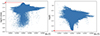 |
Fig. 1. Shown are the logarithm of the Alfvén speed (left) and the logarithm of the plasma β (right) as functions of the vertical magnetic field, as resolved in the Bifrost simulation ch024031_by200bz005 (Finley et al. 2022) at the height of the COCONUT GCM inner boundary, at ∼10 Mm. The red arrows point at the maximum computed Alfvén speed (left) and the minimum resolved plasma β (right) in this simulation. |
The values above are indirectly derived from observations, theory, or more detailed MHD simulations, so large uncertainties may exist in them. However, they do show that there is a rough consensus regarding the order of magnitude that would be expected at our inner boundary, which can be used to constrain our setup.
2.3. Numerical boundary condition constraining
From the numerical standpoint, to constrain the plasma βmin and VA, max to the values presented above, it is inappropriate to use a non-steady step function since such a function has a discontinuous first derivative which triggered numerical convergence issues in our tests. A smooth transition function should thus be designed between the homogeneous p0 and ρ0 values and the values computed from the constraints p′ and ρ′. This was achieved by implementing a double-sided hyperbolic tangent profile. For pressure, determined from βmin, we prescribed
 (1)
(1)
in which pmag is the magnetic pressure computed from the prescribed magnetic field. The double-sided hyperbolic tangent transition factor ζtan is given by
 (2)
(2)
The term Δ is positive if β < βmin (such that ζtan → 1) and negative if β > βmin (ζtan → 0). The constant dtan defines the range of β over which the transition occurs. If dtan is too small, convergence issues might occur (just like with a step function), whereas if dtan is too large, the constraining is no longer sharp and accurate. Based on the results of our numerical experiments, dtan was set to 10% of βmin. For density, constrained by the maximum Alfvén speed, we then have
 (3)
(3)
with
 (4)
(4)
Based on the results of numerical experiments, we again set dtan ∼ 10% of VA, max. Here, p′ and ρ′ are prescribed directly at the boundary. In COCONUT, the size of the ghost cells, the state (i.e. the vector of primitive variables) of which is denoted by g, and the size of the innermost domain cells, denoted by i, is the same, and thus so is the distance from their centroids to the boundary. Thus, the ghost cell state values become defined by pg = 2p′−pi and ρg = 2ρ′−ρi such that we achieve the values p′ and ρ′ exactly on the boundary.
Of course, the hyperbolic tangent profile only tends to the final values and never actually reaches them. However, thanks to the selection of such a small distance parameter, dtan ∼ 10% of VA, max and βmin, already, for instance, 10% below and above the limit values of β and VA, the prescribed boundary pressure and density are within just 0.2% percent of their target states. Given the other inherent uncertainties and inaccuracies in our boundary formulation (for instance, the magnetic field and the density field, as has been described in Brchnelova et al. (2023) and Perri et al. (2023), and the only first-order accurate interpolation used to prescribe the boundary values), such offsets are negligible. If needed, however, the value of dtan can be reduced further, though this could come at a possibly increased computational cost.
3. Results
The results were first obtained for an unconstrained simulation and then by constraining for several values of VA, max and βmin. The unconstrained simulation, as expected, produced a high-speed stream of speeds higher than 1 Mm/s; as can be seen in Figure 2 on the left. This stream is unexpected given the underlying magnetic structure, and resolved to be much hotter than what would be realistic for any such kind of structure in the solar corona (here, with well over 30 MK). The width of this stream was progressively reduced via decreasing VA, max, first to VA, max = 107 m/s in the middle and then down to VA, max = 106 m/s on the right, with the latter value roughly corresponding to what would be expected from the discussion in Section 2.2.
 |
Fig. 2. Shown are COCONUT results for the March 9, 2016, solar eclipse (CR2174), with maximum VA constraining. The inner surface shows the prescribed magnetic field, the contour plot of the radial speed (demonstrating the existence of inexplicable high-speed streams and their reduction thanks to the constraining), and the magnetic field lines over and around the active region, causing the high-speed streams plotted. |
From then on, to further reduce the strength of the stream, the β constraining was included with the results shown in Figure 3 for the values of βmin = 10−4, 10−3, 10−2, 2 ⋅ 10−2, and 5 ⋅ 10−2. For the more realistic βmin values (10−3 and 10−2 according to Gary (2001)), this stream first reaches lower speeds until it is mainly removed in the range between 10−2 ≤ βmin ≤ 2 ⋅ 10−2, without a significant alteration to the surrounding electromagnetic structures. For βmin values that are too high (2 ⋅ 10−2, 5 ⋅ 10−2), the flow field and the magnetic field lines become highly deformed.
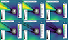 |
Fig. 3. Shown are COCONUT results for the March 9, 2016, solar eclipse (CR2174), with minimum-plasma-β constraining. The inner surface shows the prescribed magnetic field, the contour plot of the radial speed (demonstrating the existence of inexplicable high-speed streams and their removal thanks to the constraining), and the magnetic field lines over and around the active region, causing the high-speed streams plotted. |
Figure 4 depicts, for three of the selected VA, max cases, how the prescribed VA on the surface of the inner boundary changes as a result of the numerical constraining (the surface VA looking almost identical for VA, max = 107 m/s and the unconstrained case). By comparing the inner boundary surfaces visible here with those in Figure 2, it is clear that the locations of the highest VA correspond to the regions of the strongest magnetic field, as would be expected. It is also these regions that are affected by limiting VA, max, with these high values being progressively removed in Figure 4 from left to the right, and with the rest of the inner boundary VA surface being unaffected. The same is shown in Figure 5 for plasma β, with the β-unconstrained and βmin = 10−4 again looking very similar. As was the case of VA, the regions of the smallest plasma β correspond to the those where the magnetic field is the strongest, and it is only these regions where the β values are affected as we increase βmin from 10−4 at the top, left to βmin ≥ 10−2 in the bottom row.
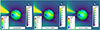 |
Fig. 4. For the March 9, 2016 solar eclipse (CR2174), the changes to the prescribed Alfvén speed VA on the inner boundary are shown for three cases as a consequence of VA, max constraining. The highest VA, max solution on the left looked the same as the unconstrained one. |
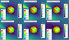 |
Fig. 5. For the March 9, 2016, solar eclipse (CR2174), the changes to the prescribed plasma β on the inner boundary are shown for six cases as a consequence of βmin constraining. The lowest βmin solution on the left looked the same as the one unconstrained with βmin, only with VA, max. |
With the selection on the limiting β and VA, one can also analyse the effects that this technique has on the assumed temperature (which is not a primitive variable in the solver, and so it must be derived from the pressure and density, with T ∝ p/ρ). Reducing VA, max means increasing the surface density, lowering the corresponding temperature. In contrast, increasing βmin means increasing the surface pressure and thus the temperature. As a result, controlling these two parameters together may be used to design the desired target temperature in the constrained regions. An example of such a calculation for a 5 G region (that corresponds to a boundary magnetic field that is very typical in our maxima simulations) with a variety of VA, max and βmin values is shown in Table 1.
Temperatures for a variety of VA, max and βmin.
Notably, with this approach, the magnetic field lines resolved over these affected regions remain mostly unaltered for the physically justifiable constraining levels. In Figure 6, the magnetic field lines over and around the region causing the inexplicable stream are shown in orange. The left-most plot corresponds to an effectively unconstrained simulation, and the other plots then show the field lines with VA constraining (middle) and VA plus β constraining (right). While the magnetic field lines over the active region are somewhat sharper in the left-most case, the magnetic connectivity and general structure of the field lines remain very similar.
 |
Fig. 6. For the March 9, 2016 solar eclipse (CR2174), the detailed magnetic field lines are plotted over and around the strong active region causing the inexplicable high-speed streams for three levels of constraining (effectively no constraining on the left, VA, max = 106 m/s in the middle and VA, max = 106 m/s with βmin = 10−2 constraining on the right). |
4. Discussion and conclusion
In this paper, we have developed and demonstrated a method to alter the pressure and density boundary condition formulations of the global coronal model COCONUT (Perri et al. 2022) to remove inexplicable features in the domain. These features stem from the fact that in the default model setup, the density and pressure are assumed to be homogeneous all across the coronal boundary surface, which is especially inaccurate in regions with stronger magnetic fields. Inappropriate density and pressure prescriptions then lead to nonphysically large Alfvn speeds and low plasma β values, affecting the plasma dynamics.
By analysing literature findings and the data from the solar atmospheric code Bifrost (Gudiksen et al. 2011), realistic orders of magnitude of the minimum and maximum constraints on the boundary β and Alfvén speed were identified, with these parameters acting as proxies to the boundary pressure (from plasma β) and density (from Alfvén speed). To ensure a smooth transition and avoid convergence issues, a double-sided hyperbolic transition profile was employed for this constraining.
Tests conducted on the 2016 solar eclipse case (March 9, CR 2174) demonstrated that VA, max constraining with the values that would be expected in the lower corona (∼106) contributed to the reduction of the radial width of the inexplicable features. Further reduction was achieved via βmin-constraining, with the most effective values being 10−3 < βmin ≤ 1 ⋅ 10−2, above which the β became nonphysically high and led to a distortion of the flow and magnetic fields. The specific values of VA, max and βmin can be chosen to achieve a specific target temperature in the regions undergoing limiting, depending on the strength of the magnetic field. It was also confirmed that for a reasonable selection of VA, max and βmin, beyond the removal of the inexplicable feature, the shape and the configuration of the magnetic field lines above the constrained regions were not significantly affected by the adopted method.
Thanks to missions such as the Solar Orbiter and the Parker Solar Probe, we can hopefully soon acquire new high-resolution observations allowing us to prescribe solar coronal conditions more accurately. Until that is the case, however, a technique such as the one presented in this paper might serve as a partial remedy to constrain global coronal models.
Acknowledgments
This research was supported by the Research Council of Norway through its Centres of Excellence scheme, project number 262622, and through grants of computing time from the Programme for Supercomputing. This work has been further granted by the AFOSR basic research initiative project FA9550-18-1-0093. The project has also received funding from the European Union’s Horizon 2020 research and innovation programme under grant agreement No 870405 (EUHFORIA 2.0). These results were also obtained in the framework of the projects C16/24/010 (C1 project Internal Funds KU Leuven), G0B5823N and G002523N (WEAVE) (FWO-Vlaanderen), V461823N (FWO-Vlaanderen), 4000134474 (SIDC Data Exploitation, ESA Prodex), and Belspo project B2/191/P1/SWiM. The resources and services used in this work were provided by the VSC (Flemish Supercomputer Centre), funded by the Research Foundation – Flanders (FWO) and the Flemish Government.
References
- Alissandrakis, C. E., & Gary, D. E. 2021, Front. Astron. Space Sci., 7, 591075 [CrossRef] [Google Scholar]
- Anfinogentov, S. A., & Nakariakov, V. M. 2019, ApJ, 884, L40 [CrossRef] [Google Scholar]
- Arge, C. N., Odstrcil, D., Pizzo, V. J., & Mayer, L. R. 2003, Conf. Proc., 679, 190 [NASA ADS] [Google Scholar]
- Baratashvili, T., Brchnelova, M., Linan, L., Lani, A., & Poedts, S. 2024, A&A, 690, A184 [NASA ADS] [CrossRef] [EDP Sciences] [Google Scholar]
- Bourdin, P.-A. 2017, ApJ, 850, L29 [NASA ADS] [CrossRef] [Google Scholar]
- Bourdin, P.-A. 2020, Geophys. Astro. Fluid, 114, 235 [CrossRef] [Google Scholar]
- Bourdin, P.-A., Bingert, S., & Peter, H. 2013, A&A, 555, A123 [NASA ADS] [CrossRef] [EDP Sciences] [Google Scholar]
- Brchnelova, M., Kuźma, B., Perri, B., et al. 2022a, ApJS, 263, 18 [NASA ADS] [CrossRef] [Google Scholar]
- Brchnelova, M., Zhang, F., Leitner, P., et al. 2022b, JPP, 88, 905880205 [Google Scholar]
- Brchnelova, M., Kuźma, B., Zhang, F., Lani, A., & Poedts, S. 2023, A&A, 676, A83 [NASA ADS] [CrossRef] [EDP Sciences] [Google Scholar]
- Doschek, G. A., Feldman, U., Laming, J. M., et al. 1998, ApJ, 507, 991 [NASA ADS] [CrossRef] [Google Scholar]
- Finley, A. J., Brun, A. S., Carlsson, M., et al. 2022, A&A, 665, A118 [NASA ADS] [CrossRef] [EDP Sciences] [Google Scholar]
- Gary, G. A. 2001, Sol. Phys., 203, 71 [Google Scholar]
- Gombosi, T. I., van der Holst, B., Manchester, W. B., & Sokolov, I. V. 2018, Liv. Rev. Sol. Phys., 15, 4 [CrossRef] [Google Scholar]
- Gudiksen, B. V., Carlsson, M., Hansteen, V. H., et al. 2011, A&A, 531, A154 [NASA ADS] [CrossRef] [EDP Sciences] [Google Scholar]
- Hollweg, J. V. 1978, Rev. Geophys. Space Phys., 16, 689 [CrossRef] [Google Scholar]
- Iwai, K., Shibasaki, K., Nozawa, S., et al. 2014, EPS, 66, 149 [Google Scholar]
- Kuźma, B., Brchnelova, M., Perri, B., et al. 2023, ApJ, 942, 31 [CrossRef] [Google Scholar]
- Linker, J., Mikic, Z., Biesecker, D. A., et al. 1999, J. Geophys. Res. Space Phys., 104, 9809 [NASA ADS] [CrossRef] [Google Scholar]
- Mikic, Z., & Linker, J. A. 1996, Conf. Proc., 382, 104 [NASA ADS] [Google Scholar]
- Mikic, Z., Linker, J. A., Schnack, D. D., Lionello, R., & Tarditi, A. 1999, PoP, 6, 2217 [Google Scholar]
- Parenti, S., Réville, V., Brun, A. S., et al. 2022, ApJ, 929, 75 [NASA ADS] [CrossRef] [Google Scholar]
- Perri, B., Leitner, P., Brchnelova, M., et al. 2022, ApJ, 936, 19 [NASA ADS] [CrossRef] [Google Scholar]
- Perri, B., Kuźma, B., Brchnelova, M., et al. 2023, ApJ, 943, 124 [NASA ADS] [CrossRef] [Google Scholar]
- Pomoell, J., & Poedts, S. 2018, JSWSC, 8, A35 [NASA ADS] [Google Scholar]
- Réville, V., Brun, A. S., Matt, S. P., Strugarek, A., & Pinto, R. F. 2015, ApJ, 798, 116 [Google Scholar]
- Rosner, R., Tucker, W. H., & Vaiana, G. S. 1978, ApJ, 220, 643 [Google Scholar]
- Samara, E., Pinto, R. F., Magdalenić, J., et al. 2021, A&A, 648, A35 [EDP Sciences] [Google Scholar]
- Scherrer, P. H., Schou, J., Bush, R. I., et al. 2012, Sol. Phys., 275, 207 [Google Scholar]
- Shi, T., Manchester, W., Landi, E., et al. 2022, ApJ, 928, 34 [NASA ADS] [CrossRef] [Google Scholar]
- van der Holst, B., Sokolov, I. V., Meng, X., et al. 2014, ApJ, 782, 81 [Google Scholar]
All Tables
All Figures
|
Fig. 1. Shown are the logarithm of the Alfvén speed (left) and the logarithm of the plasma β (right) as functions of the vertical magnetic field, as resolved in the Bifrost simulation ch024031_by200bz005 (Finley et al. 2022) at the height of the COCONUT GCM inner boundary, at ∼10 Mm. The red arrows point at the maximum computed Alfvén speed (left) and the minimum resolved plasma β (right) in this simulation. |
| In the text | |
|
Fig. 2. Shown are COCONUT results for the March 9, 2016, solar eclipse (CR2174), with maximum VA constraining. The inner surface shows the prescribed magnetic field, the contour plot of the radial speed (demonstrating the existence of inexplicable high-speed streams and their reduction thanks to the constraining), and the magnetic field lines over and around the active region, causing the high-speed streams plotted. |
| In the text | |
|
Fig. 3. Shown are COCONUT results for the March 9, 2016, solar eclipse (CR2174), with minimum-plasma-β constraining. The inner surface shows the prescribed magnetic field, the contour plot of the radial speed (demonstrating the existence of inexplicable high-speed streams and their removal thanks to the constraining), and the magnetic field lines over and around the active region, causing the high-speed streams plotted. |
| In the text | |
|
Fig. 4. For the March 9, 2016 solar eclipse (CR2174), the changes to the prescribed Alfvén speed VA on the inner boundary are shown for three cases as a consequence of VA, max constraining. The highest VA, max solution on the left looked the same as the unconstrained one. |
| In the text | |
|
Fig. 5. For the March 9, 2016, solar eclipse (CR2174), the changes to the prescribed plasma β on the inner boundary are shown for six cases as a consequence of βmin constraining. The lowest βmin solution on the left looked the same as the one unconstrained with βmin, only with VA, max. |
| In the text | |
|
Fig. 6. For the March 9, 2016 solar eclipse (CR2174), the detailed magnetic field lines are plotted over and around the strong active region causing the inexplicable high-speed streams for three levels of constraining (effectively no constraining on the left, VA, max = 106 m/s in the middle and VA, max = 106 m/s with βmin = 10−2 constraining on the right). |
| In the text | |
Current usage metrics show cumulative count of Article Views (full-text article views including HTML views, PDF and ePub downloads, according to the available data) and Abstracts Views on Vision4Press platform.
Data correspond to usage on the plateform after 2015. The current usage metrics is available 48-96 hours after online publication and is updated daily on week days.
Initial download of the metrics may take a while.