| Issue |
A&A
Volume 676, August 2023
|
|
|---|---|---|
| Article Number | A83 | |
| Number of page(s) | 13 | |
| Section | Numerical methods and codes | |
| DOI | https://doi.org/10.1051/0004-6361/202346788 | |
| Published online | 11 August 2023 | |
The role of plasma β in global coronal models: Bringing balance back to the force
1
Centre for Mathematical Plasma Astrophysics, KU Leuven,
Celestijnenlaan 200B,
3001
Leuven, Belgium
e-mail: This email address is being protected from spambots. You need JavaScript enabled to view it.
2
Shenzhen Key Laboratory of Numerical Prediction for Space Storm, Institute of Space Science and Applied Technology, Harbin Institute of Technology,
Shenzhen
518055, PR China
3
Key Laboratory of Solar Activity and Space Weather, National Space Science Center, Chinese Academy of Sciences,
Beijing
100190, PR China
4
Institute of Physics, University of Maria Curie-Skłodowska,
ul. Radziszewskiego 10,
20-031
Lublin, Poland
Received:
2
May
2023
Accepted:
8
June
2023
Abstract
Context. COolfluid COrona uNstrUcTured (COCONUT) is a global coronal magnetohydrodynamic (MHD) model that was recently developed and will soon be integrated into the ESA Virtual Space Weather Modelling Centre (VSWMC). In order to achieve robustness and fast convergence to a steady state for numerical simulations with COCONUT, several assumptions and simplifications were made during its development, such as prescribing filtered photospheric magnetic maps to represent the magnetic field conditions in the lower corona. This filtering leads to smoothing and lower magnetic field values at the inner boundary (i.e. the solar surface), resulting in an unrealistically high plasma β (greater than 1 in a large portion of the domain).
Aims. We aim to examine the effects of prescribing such filtered magnetograms in global coronal simulations and formulate a method for achieving more realistic plasma β values and improving the resolution of electromagnetic features without losing computational performance.
Methods. We made use of the newly developed COCONUT solver to demonstrate the effects of the highly pre-processed magnetic maps set at the inner boundary and the resulting high plasma β on the features in the computational domain. Then, in our new approach, we shifted the inner boundary to 2 R⊙ from the original 1.01 R⊙ and preserved the prescribed highly filtered magnetic map. With the shifted boundary, the boundary density and pressure were also naturally adjusted to better represent the considered physical location. This effectively reduces the prescribed plasma β and leads to a more realistic setup. The method was applied on a magnetic dipole, a minimum (2008) and a maximum (2012) solar activity case, to demonstrate its effects.
Results. The results obtained with the proposed approach show significant improvements in the resolved density and radial velocity profiles, and far more realistic values of the plasma β at the boundary and inside the computational domain. This is also demonstrated via synthetic white light imaging (WLI) and with the validation against tomography data. The computational performance comparison shows similar convergence to a limit residual on the same grid when compared to the original setup. Considering that the grid can be further coarsened with this new setup, as its capacity to resolve features or structures is superior, the operational performance can be additionally increased if needed.
Conclusions. The newly developed method is thus deemed as a good potential replacement of the original setup for operational purposes, providing higher physical detail of the resolved profiles while preserving a good convergence and robustness of the solver.
Key words: magnetohydrodynamics (MHD) / methods: numerical / Sun: corona
© The Authors 2023
 Open Access article, published by EDP Sciences, under the terms of the Creative Commons Attribution License (https://creativecommons.org/licenses/by/4.0), which permits unrestricted use, distribution, and reproduction in any medium, provided the original work is properly cited.
This article is published in open access under the Subscribe to Open model. This email address is being protected from spambots. You need JavaScript enabled to view it. to support open access publication.
1 Introduction
Space weather forecasting has gained importance in the past few decades as our society relies more and more on digital technologies and space infrastructure, both of which are fairly susceptible to space weather effects. Space weather modelling is, however, not a straightforward task due to the different environments that the solar wind and transients pass through on their way from the Sun to the Earth’s atmosphere. Typically, these different environments require different physics to be considered, and this is why software frameworks such as the ESA Virtual Space Weather Modelling Centre (VSWMC) have been developed (Poedts et al. 2020), allowing for the coupling of a chain of models to each other for forecasting purposes. The current heliospheric wind and coronal mass ejections (CMEs) evolution modelling in the VSWMC relies heavily on the Wang-Sheeley-Arge (WSA, Arge et al. 2003) -like coronal model in EUHFORIA (Pomoell & Poedts 2018), because the alternative coronal models (Wind-Predict; Réville et al. 2015 and Multi-VP; Samara et al. 2021) require substantially more CPU time. The WSA model is, however, semi-empirical and has been repeatedly shown to produce inaccurate boundary data at 0.1 AU (Samara et al. 2021). Yet, the coronal model is of great importance to space weather predictions since it is the first model on the side of the Sun, propagating the plasma field to the rest of the chain, for example to the EUHFORIA Heliosphere module (Pomoell & Poedts 2018) and the faster (AMR) version, ICARUS (Verbeke et al. 2019). Thus, any errors generated by this coronal model will spoil the prediction, regardless of the accuracy of the models that follow.
In previous work (Perri et al. 2022), we introduced COCONUT (COolfluid COronal uNstrUcTured), a global coronal modelling tool relying on ideal-MHD, which can alternatively be used to predict the plasma properties at 0.1 AU. The model was shown to produce good results when comparing the magnetic field lines with the observed streamers (see Kuźma et al. 2023) and demonstrated a competitive run time (typically 30 minutes to 4 h) on high-performance computing (HPC) setups, depending on the case complexity (Perri et al. 2022).
Despite the demonstrated suitability of COCONUT for operational purposes, more work is needed in order to improve its physical accuracy and the reliability of its results. In particular, COCONUT’s results generally display very smooth density profiles showing little response to the electromagnetic structures such as streamers, despite the fact that these streamers are resolved accurately if one considers their magnetic field lines. Here, we show that this is largely caused by the pre-processing of the magnetic maps that we used for the mentioned simulations. Since we pre-process the magnetograms to enable numerical stability and fast convergence, by significantly reducing their resolution and magnetic field strength we are also reducing the magnetic pressure within the computational domain. This causes an imbalance of forces and pressures yielding a relatively high plasma β. As a result, the force balance and thus the whole plasma dynamics are affected.
In this paper, we first briefly introduce the numerical setup of the solver in Sect. 2, including the formulation, the grid, the boundary and initial conditions. In the same section, we also discuss the magnetic field pre-processing techniques and the expected magnetic field strength at our inner boundary, showing that our default setup uses magnetic maps that are too weak. In Sect. 3, we formulate an original technique to partly mitigate these effects, consisting of placing the inner boundary further away from the Sun while preserving the weaker magnetic field. We apply this technique on three cases, consisting of a dipole, a minimum solar activity case and a maximum solar activity case with validation against synthetic white-light imaging and tomography. We also evaluate the impact on the convergence behaviour, as a good performance and robustness remain essential for the operational utility of COCONUT, and discuss implications for the future use of the solver. We conclude by summarising our findings in Sect. 4.
2 Methodology
The plasma solver COCONUT was originally introduced with the aim of becoming an alternative, efficient, MHD-based coronal model for the VSWMC (Perri et al. 2022). In this section, we first present its formulation and the default numerical setup. We then focus on the prescription and pre-processing of the magnetic field on its inner boundary, highlighting the effects it has on the validity and resolution of the simulation results.
2.1 Formulation
The global coronal model COCONUT, based on the COOLFluiD Framework (see, e.g., Lani et al. 2006; Kimpe et al. 2005; Lani et al. 2013), solves for the non-dimensional ideal-MHD equations (Yalim et al. 2011) with gravity using a fully-implicit unstructured second-order finite volume (FV) solver. The implicit nature of the steady-solver allows for CFL values much larger than 1, often into thousands in an operational setting. The MHD formulation of the default COCONUT setup is given below:
 (1)
(1)
 (2)
(2)
 (3)
(3)
 (4)
(4)
 (5)
(5)
where B is the magnetic field, V the plasma velocity, ρ the density, P the scalar pressure, g the gravitational acceleration, and E the total internal energy, and ϕ serves for hyperbolic divergence cleaning. The reference values that are used to non-dimensionalise the equations are Bref = 2.2 × 10⁻⁴ T, lref = 6.9551 × 10⁸ m, and pref = 1.6 × 10⁻¹³ kg m−3. We note that in the equations above, radiation, conduction, and heating are not included. The implementation of these terms into the solver formulation is ongoing. For the purpose of this study, we deem the baseline COCONUT formulation shown above to be sufficient since this baseline setup starts in the lower corona and resolves the magnetic structures well while also being very robust (see e.g. Kuźma et al. 2023).
Grid resolution for the simulated cases.
2.2 The grid
The grid that was used in this study corresponds to the standard grid of the COCONUT solver (see Brchnelova et al. 2022b). This grid is unstructured and based on a subdivided icosahe-dron spanning from 1.01 R⊙ to 25 R⊙, where the latter boundary was adjusted by Brchnelova et al. (2022a) to remove the outer boundary condition effects. For each of the cases shown below, a different grid resolution is used, with refinement increasing with the complexity of the flow field. The number of grid points for each case is shown in Table 1.
2.3 Default initial and boundary conditions
Since the solar wind at the outer boundary is super-fast, extrapolation from the last cell inside the domain was used at this boundary. The inner boundary conditions fully determine the flow field. These were prescribed in terms of density, pressure, velocity, and magnetic field. The magnetic field was set to represent the Br component of the magnetic map of the case that was to be studied. The density was prescribed to be 1.0 and the pressure to be 0.108, both in non-dimensional terms (Perri et al. 2022). For some cases, especially when maxima of solar activity are studied, the prescribed density might have to be locally or globally increased in order to ensure stability of the solver (see Brchnelova et al. 2023 for details). The question of the magnitude and direction of the outflow velocity that is imposed on the inner surface was discussed in detail in Brchnelova et al. (2022a), as were the initial conditions. In the following study, if the initial and boundary conditions deviate from what is indicated above, it is clearly stated.
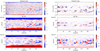 |
Fig. 1 Demonstration of pre-processing of photospheric magnetic maps (top) through spherical harmonics processing, with lmax of 30 (middle) and 15 (bottom). On the left, the magnetic map from the selected minimum of activity case (August 1, 2008 eclipse) is shown. On the right, the magnetic maps correspond to the maximum activity case (November 13, 2012 eclipse). Units are in Gauss. |
2.4 Magnetic map pre-processing
Photospheric magnetograms generally have very high resolution and very high magnetic field strengths. Due to the large gradients and the high local values of the magnetic field, unprocessed magnetograms are generally unpractical for global coronal simulations because they would easily affect their robustness and performance. In order to make them suitable for space weather forecasting runs, a smoothing is applied, and this is frequently justified by the fact that the magnetic field is expected to be lower in the upper chromosphere and corona than in the photosphere (see e.g. the analysis of Joshi et al. 2017 for sunspots). Therefore, our typical approach (see e.g. Kuźma et al. 2023) is to pre-process the photospheric magnetic maps through spherical harmonics, where the high spherical harmonics beyond a certain lmax are filtered away. For a demonstration, we refer the reader to Fig. 1, where the separate magnetic maps correspond to the same original photospheric magnetogram shown on the top, but have different levels of lmax. Both the magnetic field strength and the resolution diminish as lmax decreases. In our setting, for rapid convergence, we generally consider lmax = 15 or 30, depending on whether the case corresponds to a minimum or maximum of solar activity, respectively. In the following, HMI magnetograms are used for our simulations unless stated otherwise (Perri et al. 2023).
Typically, this results in maximum magnetic field strength values in the range of 1–2 G at the inner boundary for minima cases and 10–15 G for maxima cases. Such values allow for a smooth run of the simulation, converging in times that are feasible for operational purposes (Perri et al. 2022). While the convergence performance is clearly one of the most important aspects of the solver as it is meant to become a part of a space weather forecasting tool chain, this limited strength of the magnetic field results in a decrease of the magnetic pressure and thus influences the level to which the plasma is capable of following the magnetic field lines. While it is expected that the magnetic field and its gradients will diminish to a certain extent between the photosphere and the lower corona, this limit of lmax has so far mostly been set based on the operational performance of the solver, not on the physical evidence of the maximum magnetic field strength expected at the inner boundary.
2.5 Realistic B-field strength in the lower corona and its effects
We first look at the magnetic field that should be prescribed at the lower boundary. While we do not know the exact magnetic field strength and evolution in the lower corona, there are several ways in which this magnitude can be estimated from observations and simulations. A quite exhaustive review was performed by Alissandrakis & Gary (2021) summarising the magnetic field strength evolution with height for active regions through different radio methods, such as polarisation reversal, metric bursts, or Faraday rotation, as summarised in Fig. 14 of the referenced work. While there is quite a spread in the data due inclusion of the different techniques, it is clear that the estimated maximum magnetic field strength at 1.01 R⊙ should be much higher than the current 1–15 G used in our simulations (with the zebra pattern and the Dulk-McLean relation showing a range of 50 G to 200 G).
For a demonstration of this issue, we considered a case of a converged 2008 solar eclipse simulation. In Fig. 2, we show the radial velocity profile with magnetic field lines (left) and the density profile (right), which clearly showcase the difficulty that the plasma has in following the magnetic field lines. This insufficiency also presents itself in the evaluation of the plasma β. For the same 2008 case, we plotted the plasma beta in the flow field (left) and on the inner boundary (right) in Fig. 3. If we take into account the estimations for plasma β, β = nkT/(B2/2µ0), from Fig. 3 of Gary (2001), we would be expecting the plasma β at the location of 1.01 R⊙ to be below 0.01. While one would expect this value to be very large along streamers where the magnetic field approaches very small values (i.e. the bright yellow regions), a sufficiently low plasma β is clearly not achieved, even in the rest of the domain or at the boundary. This means that the thermal pressure is too large compared to the magnetic pressure and explains why the resolved plasma dynamics lacks strong electromagnetic features.
 |
Fig. 2 Resolved profiles of 2008 minimum solar activity case. The left panel shows the magnetic field lines (in white), with the background contours indicating the radial velocity profile. The right panel shows the corresponding, largely radial, density profile. |
 |
Fig. 3 Plasma β in the domain (left) and on the inner surface (right) for the 2008 minimum solar activity case. |
3 Results with a shifted boundary
From the discussion above, it is clear that the magnetic field currently prescribed for operational COCONUT runs is much smaller than what is realistic at that location in the low corona, at least when it comes to the active regions generally giving rise to strong features in the flow field. It is also clear that this assumption leads to deviations from what is physical in the simulation results. However, from our previous numerical experiments, even with increased limiting, prescribing a much higher magnetic field leads to deteriorated convergence and run-time performance. Therefore, an alternative solution should remedy this issue for operational usage.
In order to improve the physicality of our simulations without prescribing higher magnetic fields, however, we can invert the logic. Looking at the review paper of Alissandrakis & Gary (2021), Fig. 14, the magnetic field strength of 1–10 G that we assume would be expected roughly at a height of 1 R⊙ from the photosphere. Thus, we simply shifted the inner boundary to this distance (2 R⊙ in total).
In order to be consistent, when shifting the inner boundary, we must adjust not only the magnetic field but also the other boundary conditions. To this end, we considered the profiles from the work of Lemaire & Katsiyannis (2021). According to Fig. 1 of this paper, with the base equatorial density at the solar surface of around 1087 cm−3 (8.4 × 10⁻¹³ kg m−3), at 1 R⊙ height from the photosphere this number density drops to 5.3 × 10⁻¹⁵ kg m−3. The pressure was adjusted accordingly.
We note that there are topological consequences resulting from the fact that we shifted the location at which we prescribe the magnetic field. These are discussed in Sect. 3.3.
 |
Fig. 4 Density profiles of simulated magnetic dipole with original setup (left: boundary located at 1.01 R⊙) and new setup (right: boundary located at 2.0 R⊙). The prescribed magnetic field is the same for both cases and shown on the inner boundary using the colour bar on the left. The resolved density profile is indicated using the colour bar on the right. |
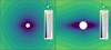 |
Fig. 5 Radial velocity profiles of simulated magnetic dipole with original setup (left: boundary located at 1.01 R⊙) and new setup (right: boundary located at 2.0 R⊙). |
3.1 Dipolar case
First, we applied this logic to the case of a dipole to see how this modification affects the density field in a simple case. In Fig. 4, the density profiles of the original approach (on the left) and the shifted-boundary approach (on the right) are demonstrated. The surface magnetogram sphere in the middle in the red and blue colour map demonstrates that while the inner sphere is 1.01 R⊙ on the left and 2 R⊙ on the right, the magnetic field that is prescribed on it is the same, following the logic outlined above. The figure shows that the new approach leads to more pronounced density features around the equator, as would be expected from a case in which the electromagnetic forces and the magnetic pressure are more dominant compared to the gravity and the thermal pressure.
A similar observation can be made from plotting the radial velocity (Fig. 5), where again the original case is on the left and the shifted-boundary case on the right. Despite the fact that the range for the velocity magnitude in the domain remains the same, the equatorial streamers are much better shaped in the shifted-boundary case. In order to verify whether these observed changes are significant enough to also improve the simulations based on real magnetic maps, this approach was next also tested for a solar minimum and a solar maximum case.
3.2 Minimum and maximum activity cases
In applying this new approach to real cases, we started with the 2008 eclipse case that was previously introduced. We repeated the steps described for the dipole, shifting the inner boundary to 2 R⊙ and adjusting the boundary density and pressure accordingly while keeping the same prescribed magnetic map. The results for this and the original approach are shown in Fig. 6, which demonstrates that the density profile in the case of the shifted-boundary approach (right) is much better developed compared to the original (left).
A comparison of the radial velocity profile in Fig. 7, for the original simulation (left) and the shifted-boundary simulation (right), portrays a much higher level of detail for the latter. Based on the investigation of the shape of the magnetic field lines in the bottom panels of Fig. 7, which were already validated in Kuźma et al. (2023), it can be concluded that the added detail is physical. Considering that both simulations are resolved using the same grid refinement and the same scheme, this added level of detail is fairly significant and can help us reduce the computational cost of predictions by allowing us to potentially run simulations on even coarser grids.
This enhancement can also be understood as an improvement in matching the correct plasma β both at the inner boundary and in the flow field. The plasma β for the shifted-boundary simulation is shown in Fig. 8. If we investigate the plasma β in Fig. 3 of Gary (2001), over the active regions at the distance of 2 R⊙, we would expect plasma β values in the range of 0.3 to around 15 (non-dimensional). This is similar to the values obtained at the inner boundary with this approach. In the rest of the flow field, we would expect the value to keep increasing up to more than 0.1 at the outer boundary, which again is satisfied.
From the analysis above and revisiting the ideal MHD formulation, it is possible to recognise the following three ways in which shifting the inner boundary helps the solver to arrive at a more physical and a better resolved flow field. Firstly, by assuming a smaller boundary density at 2 R⊙, the thermal pressure and the gravity are automatically reduced while the magnetic pressure is kept the same. Secondly, by increasing the distance from the centre of the Sun, the gravity force is reduced even further. Thirdly, as the boundary is now placed on 2 R⊙, the higher plasma β is more physical.
To further demonstrate how the more detailed density profile leads to more physical results, synthetic WLI were generated from these simulations for both cases. For synthetic WLI, we followed the spherically symmetric inversion method of Billings (1966) in order to compute, for each point, the polarised brightness integrated along the line of sight (LOS) as
 (6)
(6)
where
 (7)
(7)
![Mathematical equation: $B\left( r \right) = - {1 \over 8}\left[ {1 - 3\,{{\sin }^2}{\rm{\Omega - co}}{{\rm{s}}^2}{\rm{\Omega }}\left( {{{1 + 3{{\sin }^2}{\rm{\Omega }}} \over {\sin {\rm{\Omega }}}}} \right)\ln \left( {{{1 + \sin {\rm{\Omega }}} \over {\cos {\rm{\Omega }}}}} \right)} \right],$](/articles/aa/full_html/2023/08/aa46788-23/aa46788-23-eq8.png) (8)
(8)
and  with r2 = s2 + p2.
In the expressions above, s represents the path distance over which the integration is carried out, ρ the perpendicular distance to the solar disc, and u the limb-darkening coefficient, which was set to 0.5 in the present study.
The box over which the ray tracing was performed was set to 3.5 R⊙ × 3.5 R⊙ × 3.5 R⊙ with 250 × 250 rays, originating from uniformly distributed points. A convergence study on the size of the domain and number of rays revealed that these values were sufficient to accurately capture the brightness features (or lack thereof).
The results of WLI are shown in Fig. 9, where the original approach is shown on the left, the new approach on the right, and the observation in the middle. It should be noted that it is not the intention of the authors to have the reader thoroughly compare the exact contrast, location, and geometry of the visible synthetic WLI features with the WLI observations since it is known that the inclusion of additional physical terms, which are currently neglected, will further affect the positioning and shape of these streamers (and hence such a detailed comparison with the real physics would be unfair for both approaches). The contrast and definition in the shown WLI observation is also achieved through sophisticated post-processing, which has not yet been implemented in our synthetic WLI image generation. However, the observation is included nevertheless to provide an indication of where one should expect intensity enhancements for this specific solar activity level and magnetic field configuration. In the original case (left), no features are visible, which is why the comparison with the eclipse pictures through WLI was previously impossible for COCONUT simulation results. On the right, for the new approach, enhancements of intensity are seen in the locations where the streamers are located shown in Fig. 7, in similar locations to the enhancements seen in the observation in the middle. As stated above, it is expected that the inclusion of more physics in our model, such as coronal heating approximation, wave turbulence terms, conduction and radiation, various WLI filters, and post-processing will enhance the features even further.
Besides WLI, another means of validating (at least qualitatively) the shape of the resolved density profiles for cases of minimum solar activity is tomography. From tomography, the profiles of electron density can be derived at various distances from the Sun, generally between 4 and 8 R⊙. We used the coronagraph image data at 4.4 R⊙ of Morgan (2015) after having processed it through a spherical harmonic-based regularised inversion method (Morgan 2019) and further refinement steps (Morgan & Cook 2020).
The tomography for the date of the minimum of activity case is shown in Fig. 10 on the left. In the middle of the same figure, the synthetic tomographic image was created using the original setup with a weak magnetic field applied to 1.01 R⊙. On the right, the synthetic tomographic image was generated for the new approach, with the boundary shifted to 2 R⊙. It is clear that the new approach produces a greater level of detail which is also generally in agreement with the actual observation, despite the fact that the model is still only polytropic.
Next, we applied this approach to a case of maximum of solar activity to demonstrate that this methodology can also be used for more complex cases. Here, we took the magnetic map of the previously mentioned 2012 eclipse and repeated the same processes as for the minimum case above.
The resulting density profiles for the original approach (left) and the shifted-boundary simulation (right) are shown in Fig. 11, again showing a much better development of the density profile, following the magnetic lines in the domain.
Similarly, the synthetic WLI were generated for comparison through the same method as outlined above. Synthetic WLI and the observation of the corresponding solar eclipse are shown in Fig. 12, demonstrating much more pronounced brightness features for the new approach compared to the original, located in the regions of streamers and density enhancements.
While it is possible to somewhat improve the features of the maxima cases by using higher resolution magnetograms using the original setup with adjustments in the divergence cleaning method, these oftentimes take much longer to converge, lead to non-physically high-velocity patches, or generate unstable features that prevent the simulation from meeting the residual criteria for convergence. Based on our numerical experiments, the new approach with the shifted boundary does not encounter these problems.
 |
Fig. 6 Density profiles of 2008 minimum solar activity case with original setup (left: boundary located at 1.01 R⊙) and new setup (right: boundary located at 2.0 R⊙). |
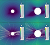 |
Fig. 7 Profiles of the 2008 minimum solar activity case with the original setup (left, boundary located at 1.01 R⊙) and the new setup (right, boundary located at 2.0 R⊙). The top two panels show the radial velocity profiles alone, while the bottom panels also overlay the magnetic field lines (in white) to help ascertain how well the plasma flow follows them. |
 |
Fig. 8 Plasma β in the domain (left) and on the prescribed surface (right) for the 2008 minimum solar activity case, as resolved using the new approach of shifting the boundary to 2 R⊙. |
 |
Fig. 9 Synthetic WLI for 2008 minimum solar activity case using density profiles from the original approach (left: boundary located at 1.01 R⊙), the new setup (right: boundary located at 2.0 R⊙), and the corresponding eclipse observation (© 2008 Alson Wong) in the middle. |
 |
Fig. 10 Comparison of tomography measurement of 2008 minimum solar activity case (left) from Morgan et al. with synthetic tomography using the density profiles from the original approach (middle: boundary located at 1.01 R⊙) and the new setup (right: boundary located at 2.0 R⊙). |
3.3 The validity of the prescribed B-field strength at 2 R⊙
While prescribing a filtered photospheric magnetic field at 2 R⊙ might be more realistic in terms of the magnetic field strength and gradients present in it, the fact that the loop footpoints are shifted by one solar radius might change the magnetic field topology (see Fig. 13). In the figure, the original ‘true’ footpoints of a given loop (solid orange arc) are located on the 1 R⊙ boundary (solid circle) in blue points. As this loop moves to the region of 2 R⊙ (dashed circle), the imagined footpoints would move to the red points. However, by simply prescribing the same magnetic field at 2 R⊙, we artificially move the footpoints to the green points through a simple linear upscaling (dotted black lines), thus making the structure larger.
In addition, some of the original 1 R⊙ loops might be small enough that they do not even extend to the distance of 2 R⊙. Obviously, by using the same magnetogram as for 1 R⊙ at 2 R⊙, these small loops will still form at this distance.
There are two implications of this. Firstly, the modelled loops might end up being larger with a different geometry, depending on their position and shape. Secondly, ‘spurious’ loops might exist close to the 2 R⊙ surface, even though their extent would otherwise be limited a distance of much less than 2 R⊙.
Despite this, as shown in the previous section, we still get much better profiles when it comes to, for example, synthetic tomography, indicating sharper and more accurate density features further away from the Sun. There are several reasons why this is the case. Firstly, more pronounced (upscaled) electromagnetic structures and lower dissipation mean that the numerical reconnection in the streamers and current sheets occurs much further away from the star, and in turn the resulting plasma features are much better pronounced as they extend into the rest of the domain. Secondly, despite the fact that the geometry and size of the loop might be affected by the above-mentioned reasons close to the inner surface, the general position of the apex of the loop is still sufficiently accurate to create density enhancements in the right places. Finally, what matter for space weather forecasting are the conditions at 0.1 AU, not those at 2 R⊙; thus, the effect of the inaccuracies close to the surface is diminished.
The above points are demonstrated in Fig. 14, where the Br features at the 5 R⊙ surface are shown for both simulated cases with both methods. It is clear that despite the different treatment of the inner boundary and different resulting velocity and density profiles in the domain, the magnetic field structure further away from the Sun looks very similar thanks to premature reconnection and the fact that the loop apexes in the new approach are still positioned at the right places. The only difference comes in terms of the magnitude of the B-field, which can however be expected since in the new approach, the same magnetic field strength is prescribed at a larger distance into the domain.
While this definitely makes it difficult to use the results of these simulations for detailed modelling of the behaviour of the coronal loops and other structures close to the star, thanks to the reasons mentioned above, we believe that this upscaling of the electromagnetic features might still be a suitable technique for improving space weather forecasting.
An alternative interpretation of the results that solves this problem exploits the non-dimensional nature of the MHD equations. Indeed, the results of the shifted-boundary case with the larger grid can be interpreted as the results computed on the original 1 R⊙ domain with a decreased boundary density, pressure, and gravity. In that case, the only parameter that changes between the two simulations in practice is the reference length, which is the reason why the gravitational force must be downscaled. In both cases, as also numerically verified, the results look exactly the same and for the 2008 minimum case, the corresponding Vr field is shown in the left-hand side plot of Fig. 15. However, with the 2 R⊙-boundary approach, it is implied that the features shown in the left plot of Fig. 15 correspond to the features that would originate from the 2 R⊙ boundary. In contrast, if we assume that the simulation is solved on the original 1 R⊙ grid but with an artificially decreased thermal pressure and gravity, the features shown in the left plot of Fig. would be assumed to originate from a 1 R⊙ boundary, and the features around the 2 R⊙ surface in the same domain would look like the features depicted in the right plot of Fig. 15. The fact that the features are much larger around the 2 R⊙ surface on the left (according to the original interpretation) compared to the 2 R⊙ surface (according to the alternative interpretation) on right further demonstrates the upscaling discussed above.
The question then concerns which one of these interpretations is more accurate and, therefore, whether the physical scale of the domain should be doubled in our simulations or not. On one hand, the latter interpretation does not face the upscaling problem and resolves sharp features with an appropriate plasma β close to the surface of the Sun. On the other hand, the former interpretation assumes a correct thermal pressure near the surface and a correct gravitational force. Considering that the scaled-down gravitational forces influence density profiles over the entire domain and hence lead to incorrect density gradients especially further away from the Sun where gravity dominates (and where the solution would be extracted for coupling to heliospheric software), the former interpretation is preferred. This means that when deriving the physical interpretation of the simulation results, we assume that the inner boundary is at the distance of 2 R⊙.
 |
Fig. 11 Density profiles of 2012 maximum solar activity case with original setup (left: boundary located at 1.01 R⊙) and new setup (right: boundary located at 2.0 R⊙). |
 |
Fig. 12 Synthetic WLI for 2012 maximum solar activity case using density profiles from original approach (left: boundary located at 1.01 R⊙), new setup (right: boundary located at 2.0 R⊙), and corresponding eclipse observation (© 2012 Constantine Emmanouilidi, Miloslav Druckmuller; in the middle). |
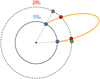 |
Fig. 13 Effects of prescribing the magnetic field at 2 R⊙ (dashed black circle) instead of 1 R⊙ (solid black circle) on the loop size and geometry (orange solid line). |
 |
Fig. 14 Comparison of resulting Br structures of the different approach at 2 R⊙ for 2008 (left two) and for 2012 (right two). |
 |
Fig. 15 Comparison of the two interpretations of the adopted approach. Both sub-figures show the radial velocity profile. The left plot shows the general result of the simulation, where the inner boundary can represent either a 2 R⊙ or a 1 R⊙ surface. On the right, the plot shows where the 2 R⊙ surface would be located if the left plot’s boundary were at 1 R⊙. |
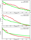 |
Fig. 16 Comparison of convergence based on Vx residual for original setup (red) and new setup (green) in dipole case (top), minimum solar activity case (middle), and maximum solar activity case (bottom). |
3.4 Convergence
Lastly, it is also essential to discuss convergence of the setups, since the primary purpose of the COCONUT solver is to be integrated into operational model chains within VSWMC for space weather forecasting. The cases presented above (dipole, 2008 minimum and 2012 maximum) were run with a constant CFL set to 1, both with the original setting and with the boundary shifted to 2 R⊙ in order to fairly determine how the residual evolves over time and when it reaches the lower pre-set limit. The simulations were run using the same grid resolution, partitioning, number and type of cores on the Flemish Supercomputer Centre. The residual chosen for monitoring was the Vx residual (the x component of the velocity), since the residual curves show its non-dimensional absolute value and these value ranges were, unlike density or pressure, similar for both setups. The results, with the original setup in red and shifted-boundary setup in green are shown in Fig. 16, with the top representing the dipole case, the middle the minimum-activity case, and the bottom the maximum-activity case.
From Fig. 16, it can be concluded that in all the cases, the shifted-boundary setup had a similar convergence performance when compared to the original setup at the same grid. While a constant CFL was held for a fair comparison in the aforementioned figure, this setup still allows for much steeper CFL profiles with higher CFL values (see Fig. 17, where the ρ residual is shown for the 2008 minimum case with a variable CFL run). Here, it is demonstrated that with gradually growing CFL values, a good convergence in just 1000 iterations (and roughly 1 hour of computing time on 144 cores) can be achieved for a realistic case with this method.
Considering the fact that the level of resolution in the results of the new approach is far more enhanced, the grid can be further coarsened, which will further improve the convergence time and stability. Furthermore, while for now the same grid was used for a fair comparison of convergence (where it was scaled up for the 2 R⊙ -boundary case), in operational runs, the outermost layers of the 2 R⊙ -boundary grid can be removed as they span far beyond 25 R⊙, which will lead to further performance enhancement.
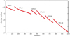 |
Fig. 17 Demonstration that rapid convergence (here ρ residual) with steep CFL profiles in just 1000 iterations is still possible with the shifted-boundary approach. |
3.5 Possible challenges of the approach
It was demonstrated that the newly applied approach leads to significantly more pronounced profiles with more realistic features compared to the original setup. It does, however, pose some limitations on the use of the code, which must also be discussed.
Firstly, clearly in this setting, we cannot accurately study the features close to the solar surface. The 1 R⊙ to 2 R⊙ region of corona cannot be studied as it is not included in the domain. The region close to the 2 R⊙ boundary cannot be used for accurate analysis either for the reasons outlined in Sect. 3.3 (e.g. the formation of loops or streamers), but this is generally considered unnecessary as this setup is meant for operational runs, not for academic research purposes. Beforehand, coronal structures were validated using solar eclipse data (derived for 1 R⊙). With this approach, coronagraph data starting from 2 R⊙ to 2.5 R⊙ could be used for that purpose.
Secondly, another potential obstacle that will have to be overcome with this setup is the fact that the majority of coronal heating term formulations to achieve bimodal wind have been developed considering the lower boundary to be at 1 R⊙, with the parameters and proportionality constants adjusted in kind. If we do, in future, switch to a 2 R⊙ inner boundary formulation, the formulation of the heating terms will have to be adjusted to produce similar results, possibly complicating the inclusion of these terms in the first place.
On the other hand, the lower solar atmosphere is highly dynamical as it is strongly affected by the turbulent convection, and this is difficult for a global coronal model to properly describe. Therefore, shifting the inner boundary could avoid the corresponding numerical and physical difficulties. For now, the demonstrated benefits appear to overcome these potential drawbacks for the polytropic MHD model.
4 Conclusions
In this paper, after having shown the effects of reducing the magnetic field strength and gradients during magnetogram preprocessing on the resolution of features in the COCONUT global coronal model simulations, we propose a simple and original method to counterbalance this simplification without losing computational performance. After a short presentation of the spherical harmonics magnetogram pre-processing and literature review, we conclude that the magnetic fields, which we generally use as an input to the COCONUT model, are unrealistically under-resolved. As demonstrated on a minimum solar activity case (2008 total eclipse), this inevitably leads to smaller electromagnetic forces and magnetic pressure with respect to gravitational forces and thermal pressure of the plasma, resulting in non-physical plasma β values and consequently leading to a lack of electromagnetic structures in density and velocity profiles. Increasing the prescribed magnetic field strength, however, deteriorates the computational performance and robustness of the code.
Therefore, we formulated an approach to mitigate this issue by placing the inner boundary further away from the star. We found that the respective magnetic fields that we currently use should be more realistic at a height of roughly 1 R⊙ from the photosphere, which means that we shifted our inner boundary to a distance of 2 R⊙, lowering the prescribed density and pressure accordingly.
By applying this new setup to the cases of a magnetic dipole, minimum solar activity (2008 total eclipse), and maximum solar activity (2012 total eclipse), we demonstrate that this approach leads to far more pronounced density profiles, correctly following the magnetic field lines. We also show that these new density profiles lead to more physical and better resolved synthetic WLI, now showcasing features despite the fact that the setup still lacks physical terms such as coronal heating, wave pressure, radiation, and conduction. For the minimum activity case, we also validate the new technique through comparison with tomography data, and it is revealed that the density profiles resulting from the new approach fit the tomography data much better, even at a distance of 4.4 R⊙.
We state that prescribing a 1 R⊙ magnetogram at 2 R⊙ might lead to larger features than what is realistic and change the shape of these features as a result. Due to the fact that for space weather forecasting we mostly focus on how these features extend in the domain and not how exactly they look close to the inner boundary, with the former being shown to be much better with the new adopted approach, we argue that despite this weakness, the proposed approach is still suitable for our purposes. It is also pointed out that due to the non-dimensional nature of the MHD equations, the new approach can also be interpreted as an approach in which we preserve the original domain starting at 1 R⊙, but in which we artificially decrease the thermal pressure and the gravity to achieve a realistic plasma β at the inner boundary. In that case, the above-mentioned problem with larger features disappears, but the prescribed thermal pressure and gravity are not representative of reality.
Finally, since COCONUT is intended for operational runs, we also evaluate its convergence with the modified inner boundary settings. From the behaviour of the velocity x-component residual, it is concluded that the convergence performance is similar to the original setup on the same grid. In addition, for the new setup, an even coarser grid can be afforded since it provides results with much better sharpness compared to the original, and with a smaller domain, it also requires fewer cells. Thus, the performance of the solver in terms of the required computational resources will only increase. Using this approach may result in the necessity to adjust our validation means in the future, focusing more on coronagraph data instead of WLI from total solar eclipses. In addition, shifting the inner boundary might make it difficult to apply some of the most popular heating terms available in literature, as these were generally developed for setups starting at 1 R⊙. This will be addressed in future work when implementing these terms into COCONUT. All in all, since this technique demonstrated superior performance and accuracy levels, it is worth considering it for operational runs despite the projected possible difficulties.
Acknowledgements
This work has been granted by the AFOSR basic research initiative project FA9550-18-1-0093. This project has also received funding from the European Union’s Horizon 2020 research and innovation program under grant agreement No. 870405 (EUHFORIA 2.0) and the ESA project “Helio-spheric modelling techniques” (Contract No. 4000133080/20/NL/CRS). These results were also obtained in the framework of the projects C14/19/089 (C1 project Internal Funds KU Leuven), G.0B58.23N (FWO-Vlaanderen), SIDC Data Exploitation (ESA Prodex-12), and Belspo project B2/191/P1/SWiM. The resources and services used in this work were provided by the VSC (Flemish Supercomputer Centre), funded by the Research Foundation – Flanders (FWO) and the Flemish Government. Wilcox Solar Observatory data used in this study was obtained via the web site http://wso.stanford.edu courtesy of J.T. Hoeksema The Wilcox Solar Observatory is currently supported by NASA Data were acquired by GONG instruments operated by NISP/NSO/AURA/NSF with contribution from NOAA. HMI data are courtesy of the Joint Science Operations Center (JSOC) Science Data Processing team at Stanford University. This work utilises data produced collaboratively between AFRL/ADAPT and NSO/NISP. Data used in this study was obtained from the following websites: WSO: http://wso.stanford.edu/synopticl.html GONG: https://gong2.nso.edu/archive/patch.pl?menutype=z HMI: http://jsoc.stanford.edu/HMI/LOS_Synoptic_charts.html GONG-ADAPT: https://gong.nso.edu/adapt/maps/
References
- Alissandrakis, C. E., & Gary, D. E. 2021, Front. Astron. Space Sci., 7, 77 [CrossRef] [Google Scholar]
- Arge, C. N., Odstrcil, D., Pizzo, V. J., & Mayer, L. R. 2003, AIP Conf. Proc., 679, 190 [Google Scholar]
- Billings, D. E. 1966, A Guide to the Solar Corona (Academic Press) [Google Scholar]
- Brchnelova, M., Kuzma, B., Perri, B., et al. 2022a, ApJS, 263 [Google Scholar]
- Brchnelova, M., Zhang, F., Leitner, P., et al. 2022b, J. Plasma Phys., 88, 905880205 [NASA ADS] [CrossRef] [Google Scholar]
- Brchnelova, M., Kuzma, B., Zhang, F., et al. 2023, arXiv e-prints [arXiv:2303.10410] [Google Scholar]
- Gary, G. A. 2001, Solar Phys., 203, 71 [NASA ADS] [CrossRef] [Google Scholar]
- Joshi, J., Lagg, A., Hirzberger, J., & Solanki, S. K. 2017, A&A, 604, A98 [NASA ADS] [CrossRef] [EDP Sciences] [Google Scholar]
- Kimpe, D., Lani, A., Quintino, T., Poedts, S., & Vandewalle, S. 2005, in Recent Advances in Parallel Virtual Machine and Message Passing Interface, eds. B. Di Martino, D. Kranzlmüller, & J. Dongarra (Berlin, Heidelberg: Springer Berlin Heidelberg), 520 [Google Scholar]
- Kuźma, B., Brchnelova, M., Perri, B., et al. 2023, ApJ, 942, 31 [CrossRef] [Google Scholar]
- Lani, A., Quintino, T., Kimpe, D., et al. 2006, Scientific Programming. Special Edition on POOSC 2005, 14, 111 [Google Scholar]
- Lani, A., Villedieu, N., Bensassi, K., et al. 2013, in AIAA 2013-2589, 21th AIAA CFD Conference, San Diego (CA) [Google Scholar]
- Lemaire, J. F., & Katsiyannis, A. C. 2021, Solar Phys., 296, 64 [NASA ADS] [CrossRef] [Google Scholar]
- Morgan, H. 2015, ApJS, 219, 23 [CrossRef] [Google Scholar]
- Morgan, H. 2019, ApJS, 242, 3 [NASA ADS] [CrossRef] [Google Scholar]
- Morgan, H., & Cook, A. C. 2020, ApJ, 893, 57 [CrossRef] [Google Scholar]
- Perri, B., Leitner, P., Brchnelova, M., et al. 2022, ApJ, 936, 19 [NASA ADS] [CrossRef] [Google Scholar]
- Perri, B., Kuźma, B., Brchnelova, M., et al. 2023, ApJ, 943, 124 [NASA ADS] [CrossRef] [Google Scholar]
- Poedts, S., Kochanov, A., Lani, A., et al. 2020, J. Space Weather Space Clim., 10, 14 [NASA ADS] [CrossRef] [EDP Sciences] [Google Scholar]
- Pomoell, J., & Poedts, S. 2018, J. Space Weather Space Clim., 8, A35 [NASA ADS] [CrossRef] [EDP Sciences] [Google Scholar]
- Réville, V., Brun, A. S., Matt, S. P., Strugarek, A., & Pinto, R. F. 2015, ApJ, 798, 116 [Google Scholar]
- Samara, E., Pinto, R. F., Magdalenić, J., et al. 2021, A&A, 648, A35 [EDP Sciences] [Google Scholar]
- Verbeke, C., Pomoell, J., & Poedts, S. 2019, A&A, 627, A111 [NASA ADS] [CrossRef] [EDP Sciences] [Google Scholar]
- Yalim, M. S., vanden Abeele, D., Lani, A., Quintino, T., & Deconinck, H. 2011, J. Comput. Phys., 230, 6136 [NASA ADS] [CrossRef] [Google Scholar]
All Tables
All Figures
|
Fig. 1 Demonstration of pre-processing of photospheric magnetic maps (top) through spherical harmonics processing, with lmax of 30 (middle) and 15 (bottom). On the left, the magnetic map from the selected minimum of activity case (August 1, 2008 eclipse) is shown. On the right, the magnetic maps correspond to the maximum activity case (November 13, 2012 eclipse). Units are in Gauss. |
| In the text | |
|
Fig. 2 Resolved profiles of 2008 minimum solar activity case. The left panel shows the magnetic field lines (in white), with the background contours indicating the radial velocity profile. The right panel shows the corresponding, largely radial, density profile. |
| In the text | |
|
Fig. 3 Plasma β in the domain (left) and on the inner surface (right) for the 2008 minimum solar activity case. |
| In the text | |
|
Fig. 4 Density profiles of simulated magnetic dipole with original setup (left: boundary located at 1.01 R⊙) and new setup (right: boundary located at 2.0 R⊙). The prescribed magnetic field is the same for both cases and shown on the inner boundary using the colour bar on the left. The resolved density profile is indicated using the colour bar on the right. |
| In the text | |
|
Fig. 5 Radial velocity profiles of simulated magnetic dipole with original setup (left: boundary located at 1.01 R⊙) and new setup (right: boundary located at 2.0 R⊙). |
| In the text | |
|
Fig. 6 Density profiles of 2008 minimum solar activity case with original setup (left: boundary located at 1.01 R⊙) and new setup (right: boundary located at 2.0 R⊙). |
| In the text | |
|
Fig. 7 Profiles of the 2008 minimum solar activity case with the original setup (left, boundary located at 1.01 R⊙) and the new setup (right, boundary located at 2.0 R⊙). The top two panels show the radial velocity profiles alone, while the bottom panels also overlay the magnetic field lines (in white) to help ascertain how well the plasma flow follows them. |
| In the text | |
|
Fig. 8 Plasma β in the domain (left) and on the prescribed surface (right) for the 2008 minimum solar activity case, as resolved using the new approach of shifting the boundary to 2 R⊙. |
| In the text | |
|
Fig. 9 Synthetic WLI for 2008 minimum solar activity case using density profiles from the original approach (left: boundary located at 1.01 R⊙), the new setup (right: boundary located at 2.0 R⊙), and the corresponding eclipse observation (© 2008 Alson Wong) in the middle. |
| In the text | |
|
Fig. 10 Comparison of tomography measurement of 2008 minimum solar activity case (left) from Morgan et al. with synthetic tomography using the density profiles from the original approach (middle: boundary located at 1.01 R⊙) and the new setup (right: boundary located at 2.0 R⊙). |
| In the text | |
|
Fig. 11 Density profiles of 2012 maximum solar activity case with original setup (left: boundary located at 1.01 R⊙) and new setup (right: boundary located at 2.0 R⊙). |
| In the text | |
|
Fig. 12 Synthetic WLI for 2012 maximum solar activity case using density profiles from original approach (left: boundary located at 1.01 R⊙), new setup (right: boundary located at 2.0 R⊙), and corresponding eclipse observation (© 2012 Constantine Emmanouilidi, Miloslav Druckmuller; in the middle). |
| In the text | |
|
Fig. 13 Effects of prescribing the magnetic field at 2 R⊙ (dashed black circle) instead of 1 R⊙ (solid black circle) on the loop size and geometry (orange solid line). |
| In the text | |
|
Fig. 14 Comparison of resulting Br structures of the different approach at 2 R⊙ for 2008 (left two) and for 2012 (right two). |
| In the text | |
|
Fig. 15 Comparison of the two interpretations of the adopted approach. Both sub-figures show the radial velocity profile. The left plot shows the general result of the simulation, where the inner boundary can represent either a 2 R⊙ or a 1 R⊙ surface. On the right, the plot shows where the 2 R⊙ surface would be located if the left plot’s boundary were at 1 R⊙. |
| In the text | |
|
Fig. 16 Comparison of convergence based on Vx residual for original setup (red) and new setup (green) in dipole case (top), minimum solar activity case (middle), and maximum solar activity case (bottom). |
| In the text | |
|
Fig. 17 Demonstration that rapid convergence (here ρ residual) with steep CFL profiles in just 1000 iterations is still possible with the shifted-boundary approach. |
| In the text | |
Current usage metrics show cumulative count of Article Views (full-text article views including HTML views, PDF and ePub downloads, according to the available data) and Abstracts Views on Vision4Press platform.
Data correspond to usage on the plateform after 2015. The current usage metrics is available 48-96 hours after online publication and is updated daily on week days.
Initial download of the metrics may take a while.