| Issue |
A&A
Volume 693, January 2025
|
|
|---|---|---|
| Article Number | A68 | |
| Number of page(s) | 12 | |
| Section | Stellar structure and evolution | |
| DOI | https://doi.org/10.1051/0004-6361/202449924 | |
| Published online | 03 January 2025 | |
The impact of disk-locking on convective turnover times of low-mass pre-main sequence and main sequence stars
1
Universidade Federal de Viçosa, Campus UFV Florestal, CEP 35690-000 Florestal, MG, Brazil
2
Depto. de Física, Universidade Federal de Minas Gerais, C.P.702, 31270-901 Belo Horizonte, MG, Brazil
3
Depto. de Engenharia Eletrônica, Universidade Federal de Minas Gerais, C.P.702, 31270-901 Belo Horizonte, MG, Brazil
⋆ Corresponding author; This email address is being protected from spambots. You need JavaScript enabled to view it.
Received:
10
March
2024
Accepted:
5
November
2024
Abstract
Aims. The impact of disk-locking on the stellar properties related to magnetic activity from the theoretical point of view is investigated.
Methods. We use the ATON stellar evolution code to calculate theoretical values of convective turnover times (τc) and Rossby numbers (Ro, the ratio between rotation periods and τc) for pre-main sequence (pre-MS) and main sequence (MS) stars. We investigate how τc varies with the initial rotation period and with the disk lifetime, using angular momentum conserving models and models simulating the disk-locking mechanism. In the latter case, the angular velocity is kept constant during a given locking time to mimic the magnetic locking effects of a circumstellar disk.
Results. The local convective turnover times generated with disk-locking models are shorter than those obtained with angular momentum conserving models. The differences are smaller in the early pre-MS, increase with stellar age, and become more accentuated for stars with M ≥ 1 M⊙ and ages greater than 100 Myr. Our new values of τc are used to estimate Ro for a sample of stars selected from the literature in order to investigate the rotation-activity relationship. We fit the data with a two-part power-law function and find the best fitting parameters of this relation.
Conclusions. The differences found between both sets of models suggest that the star’s disk-locking phase properties affect its Rossby number and its position in the rotation-activity diagram. Our results indicate that the dynamo efficiency is lower for stars that had undergone longer disk-locking phases.
Key words: convection / stars: activity / stars: evolution / stars: pre-main sequence / stars: rotation
© The Authors 2025
 Open Access article, published by EDP Sciences, under the terms of the Creative Commons Attribution License (https://creativecommons.org/licenses/by/4.0), which permits unrestricted use, distribution, and reproduction in any medium, provided the original work is properly cited.
This article is published in open access under the Subscribe to Open model. This email address is being protected from spambots. You need JavaScript enabled to view it. to support open access publication.
1. Introduction
The convective turnover time is a typical timescale for convective motions of the stars’ conductive plasma, responsible for transportation of a fraction of the energy in some types of stars, like the low-mass ones. When different parts of a magnetic star rotate differentially, the interaction between convective motions and differential rotation produces the dynamo effect (as proposed by Parker 1955) that keeps and regenerates stellar magnetic fields. In solar type stars, such fields are thought to be created and amplified at the tachocline, a thin shear layer between the radiative core and the convective envelope, first defined by Spiegel & Zahn (1992). This mechanism is supposed to drive stellar magnetic activity, expressed as a variety of observable phenomena like coronal heating, star spots, activity cycles, flares, and chromospheric and coronal emissions. For solar-like stars, it is believed that stellar magnetism and rotation are regulated by a dynamo process called the α − Ω dynamo (Mohanty & Basri 2003), in which the poloidal and toroidal field components sustain themselves through a cyclic feedback process (Nelson 2008). Nowadays, the connection between magnetic activity and rotation is well established and Skumanich (1972) was the first to suggest that the rotation-activity relation is a consequence of the dynamo action and to show that the stellar angular velocity, Ω, decreases with age as t−1/2. The rotation-magnetic activity relation has been widely used to investigate stellar magnetism. It is expressed by the relation between the stellar rotation rate (the projected rotational velocity in the line of sight or the rotation period) and some indicator of magnetic activity, such as the unsigned average large-scale surface fields (⟨|BV|⟩) or the fractional X-ray and Hα luminosities, also known as coronal (LX/Lbol) and chromospheric (LHα/Lbol) activity indicators, respectively. As shown by Noyes et al. (1984), this relationship is better understood in terms of the Rossby number, Ro (the ratio between rotation period, Prot, and the local convective turnover time, τc), than in terms of Prot. Pizzolato et al. (2003) showed for the first time that the rotation-magnetic activity relation is characterised by the existence of two distinct regions: the saturated region (formed by fast rotators – Prot ≤ 2 days) and the unsaturated region (composed by slow rotators – Prot > 2 days). LX/Lbol (or another magnetic activity indicator) increases as Ro decreases down to a saturation threshold value, Rosat ∼ 0.1, and remains constant at a saturation level, (LX/Lbol)sat ∼ 10−3, for Ro < Rosat (Wright et al. 2011, 2018). The causes of saturation are still unclear. This relation became a powerful tool to study stellar magnetism and is based on a general power-law function of the form LX/Lbol ∝ Roβ, where β is a parameter to be adjusted with observations. Values of β usually found in the literature are β = −2 (Pizzolato et al. 2003), β = −2.7 ± 0.13 (Wright et al. 2011), β = −1.38 ± 0.14 (Vidotto et al. 2014),  (Wright et al. 2018), β = −1.40 ± 0.10 (See et al. 2019), and β = −2.4 ± 0.1 (Landin et al. 2023).
Describing the rotation-magnetic activity relation in terms of the Rossby number makes clear its connection with the stellar dynamo theory, as the dynamo number (ND, the efficiency of the dynamo in the mean-field dynamo theory) is proportional to the inverse square of the Rossby number (ND ∝ Ro−2). Consequently, the dynamo efficiency increases as Ro decreases. As Ro plays an important role in the stellar magnetic activity studies, determinations of τc are of fundamental interest, since they cannot be directly measured. They can be obtained either semi-empirically (Noyes et al. 1984; Pizzolato et al. 2003) or theoretically by stellar evolution models (Kim & Demarque 1996; Landin et al. 2010). For a given stellar mass and age, the convective turnover time varies significantly with the radial location. The location mostly used in the literature to determine local convective turnover times is one half a mixing length above the base of the convective zone (Noyes et al. 1984). This standard location coincides with the tachocline for partially convective stars, but it is not suitable for fully convective stars, in which there is no tachocline. In the Mixing Length Theory, the adjustable mixing length parameter, ℓ, is scaled with the pressure scale height Hp as ℓ = αHp (α is the convection efficiency) and, during the fully convective phase, the modelled value of Hp at the base of the convective zone is very high, and so is the mixing length. Consequently, the standard location where τc should be calculated becomes larger than the stellar radius for fully convective configurations (M ≤ 0.3 M⊙ at any evolutionary stage and M > 0.3 M⊙ before developing the radiative core), making τc calculations unfeasible through this standard prescription. In order to overcome this problem, Landin et al. (2023) developed a method to obtain the location (r) where to calculate τc in terms of HP, allowing the theoretical determination of τc of fully convective stars in a self consistent way with the traditional location prescribed by Noyes et al. (1984). For ten selected ages in the range of 6.0 ≤log(t/yr)≤10.14, Landin et al. (2023) analysed how the standard location r/HP vary with stellar mass for partially convective stars, linearly fitted r/HP as a function of the stellar mass, and extrapolated it for fully convective stars. These linear fits of r/Hp as a function of mass were introduced in the ATON stellar evolution code as alternative locations to the standard τc calculation whenever r is larger than the stellar radius. Otherwise, the standard location is adopted.
Most, if not all, low-mass pre-main sequence (pre-MS) stars exhibit some manifestation of magnetic fields (Donati & Landstreet 2009). As they miss a tachocline in the beginning of their pre-MS phase, the α − Ω dynamo, which is an interface dynamo, is not supposed to be operating in this very early evolutionary phase. So, the observed magnetic activity in these stars should be produced by another kind of dynamo process, like a distributed dynamo, as suggested by Durney et al. (1993). The characteristic shape of the rotation-activity relation exhibited by main sequence (MS) stars is not observed for pre-MS stars (Flaccomio et al. 2003). The latter are seen only in the saturated region and show a considerable dispersion in magnetic activity levels (Preibisch et al. 2005). The fact that fully convective (pre-MS and MS) stars are preferably found in the saturated region, while solar-like (partially convective) stars are found in both regions, reinforces the idea that the dynamo operating in partially and fully convective stars are different. However, observations by Wright & Drake (2016) and Wright et al. (2018) indicate that partially and fully convective stars follow the same rotation-activity relation, implying that they should operate very similar rotation-dependent dynamos in which the tachocline would not be a crucial ingredient. Landin et al. (2023) present a theoretical and observational review of stellar magnetic activity in pre-MS and MS stars.
Low-mass stars in young clusters (ages ≤ 100 Myr) are known to be very active and to exhibit strong magnetic fields (specially those fast rotating), even though they do not follow the Skumanich law (Ω ∝ t−2, Alphenaar & van Leeuwen 1957). For a few million years, their magnetic field lines are supposed to be anchored in a circumstellar disk, formed during the star formation process, within a few stellar radii. The interaction between the stellar magnetic field and the disk regulates the star’s angular velocity, counteracting the tendency to spin up due to accretion of disk material of high specific angular momentum and to readjustments in the moment of inertia as the star contracts towards the MS. The magnetic torques acting on the central star during the disk lifetime transfer large amounts of its angular momentum to the disk and impose the star to rotate with a virtually constant surface angular velocity.
The observed rotation rates of stars in clusters of different ages suggest that the fast rotation phenomenon depends on mass. According to several works, such as those of Stauffer et al. (1997), Prosser et al. (1995), and Stauffer & Hartmann (1987), rapid rotation decreases slower for lower mass stars (the spin-down time scales expected for stars with M < 0.5 M⊙ are longer than those for stars with M > 1.0 M⊙). Attridge & Herbst (1992) and Choi & Herbst (1996) showed that T Tauri stars in the Orion Nebula Cluster (ONC) have a very characteristic rotation period distribution: Classical T Tauri stars (CTTS), which still accrete from a disk, have a narrow period distribution with a peak at about 8–10 days, while Weak-line T Tauri stars (WTTS), that no longer accrete from a disk, have a broader distribution showing only a tail of slow rotators. In addition, WTTS appear to rotate faster, on average, than CTTS (Henderson & Stassun 2012). ONC (1 Myr), NGC 2264 (3.5 Myr), IC 348 (2.5 Myr), and NGC 2362 (3.3 Myr) are some of the most studied young stellar clusters and all of them exhibit bimodal and dichotomic rotation period distributions. The bimodality is related to the presence of two peaks in the period distribution and the dichotomy is associated to the mass dependence of the distribution. Detailed studies of the rotation history of these clusters can be found in the literature, for example: ONC was analysed by Herbst et al. (2002), NGC 2264 was investigated by Lamm et al. (2005), Cieza & Baliber (2006) studied IC 348, Irwin et al. (2008) examined NGC 2362, the rotational properties of ONC and NGC 2264 is reviewed by Landin et al. (2016), and Landin et al. (2021) inspect such properties of IC 348 and NGC 2362. As the distribution of rotation periods in the pre-MS must evolve towards that of the MS, we have to be able to describe the process that leads from the wide distribution seen in the pre-MS to the even wider one seen in the MS. However, there is not a single model that manages to do this. In order to reproduce the evolution of stars that reach the MS with the highest rotation rates (near their breakup velocities), one should consider an evolution conserving angular momentum during all the pre-MS phase. On the other hand, to yield the rotation of stars spinning with a small fraction of their breakup velocities, one should consider that these stars are locked to their disks for a given time, keeping their angular velocities constant, and only after the locking phase they are released to spin up conserving angular momentum. Landin et al. (2016) present a theoretical and observational review of angular momentum evolution of pre-main sequence stars.
In this work, we use the ATON stellar evolution code to investigate the influence of the disk-locking mechanism on local convective turnover times (consequently, on the Rossby numbers) and in the rotation-magnetic activity relation itself. Observational data of rotation periods, fractional X-ray luminosities, and unsigned average large-scale surface magnetic fields from Vidotto et al. (2014) are used to constrain our models.
In Section 2, we briefly describe the ATON code and the input parameters used in this work. Section 3 presents and discusses our results on convective turnover times and convective velocities obtained with disk-locking and angular momentum conserving models. Our new theoretical local convective turnover times are compared to those existing in the literature and observational data are used to test our theoretical results in Section 4. Finally, Section 5 presents our conclusions.
2. Models and input physics
In the ATON code version used in this work, convection is treated according to the traditional Mixing Length Theory (Böhm-Vitense 1958), with the parameter representing the convection efficiency set as α = 2. Surface boundary conditions are obtained from non-grey atmosphere models (Allard et al. 2000) with a match between surface and interior at an optical depth of 10. We use the opacities reported by Iglesias & Rogers (1993) and Alexander & Ferguson (1994) and the equations of state from Rogers et al. (1996) and Mihalas et al. (1988). We assume that the elements are mixed instantaneously in convective regions. Our tracks start from a fully convective configuration with central temperatures in the range 5.35 < log10(Tc/K) < 5.70, follow deuterium and lithium burning, and end at the MS configuration, as discussed in Landin et al. (2006), who also presented a detailed discussion about the zero point ages of stellar models.
We generate two sets of models. In the first (hereafter AMC models), we consider conservation of angular momentum throughout all stellar evolution. In the second set (hereafter DL models), we simulate the disk-locking mechanism, by considering an evolution with constant angular velocity during the first evolutionary stages followed by conservation of angular momentum. In these models, the star-disk interaction treatment is not included in the code, and its effects on the stellar rotation are only mimicked by locking it for a while (Landin et al. 2016).
For AMC models, the initial angular momentum of each model is obtained according to the Kawaler (1987) relation1
 (1)
(1)
These initial angular momenta correspond to periods of ∼15 days for a 0.1 M⊙ model and ∼418 days for a 1.2 M⊙ model.
For DL simulating models, the initial angular momentum corresponds to the locking period, Plock, of ∼8 days2 based on the period distribution of CTTS in the ONC presented by Herbst et al. (2002). To investigate the effect of using different locking periods on τc, we ran some additional DL models with Plock = 400 days. The disk lifetimes, Tdisk, used in this work are 1 and 3 Myr, because according to Monsch et al. (2023), the majority of circumstellar disks dissipate after ∼1–3 Myr.
The evolutionary tracks were computed in the mass range of 0.1 to 1.2 M⊙ (in 0.1 M⊙ steps). We adopt the solar chemical composition (X = 0.7155 and Z = 0.0142) by Asplund et al. (2009). More details on the physics of the ATON models are given by Landin et al. (2006, 2023).
The current version of the ATON code allows for choosing among three rotational schemes (Mendes et al. 1999): (1) rigid body rotation throughout the whole star, (2) local conservation of angular momentum in the whole star (which leads to differential rotation), and (3) local conservation of angular momentum in radiative regions plus rigid body rotation in convective regions. Internal redistribution of angular momentum and angular momentum loss by stellar magnetised winds are implemented in the ATON code only for rotational scheme 3. However, there is observational evidence that the Sun’s radiative core rotates as a solid body and the convective envelope rotates differentially, opposite to scheme 3 (Thompson et al. 2003). Here, our rotating models were generated according to scheme 1, because this is the only rotational scheme for which disk-locking mechanism is implemented in the ATON code. We leave for the future the implementation of a 4th rotational scheme with a rotational profile closer to that of the Sun and disk-locking mechanism for all rotational schemes.
3. Theoretical results
By using the version of the ATON code described in Landin et al. (2023), we follow the evolution of local convective turnover times from the pre-MS to the beginning of the MS for 0.1–1.2 M⊙ stars and tabulate them together with the corresponding evolutionary tracks. Table 1 presents the 1 M⊙ DL model (Plock ∼ 8 days and Tdisk = 3 Myr) as an example of such tables. For DL models, rotation periods start from the value given by the Plock parameter, are kept constant during the first million years (according to the Tdisk parameter), and then evolve considering conservation of angular momentum from this time on. For models considering angular momentum conservation during all stages of evolution, the initial rotation periods are obtained from the initial angular momenta given in Eq. (1).
Evolutionary track for 1 M⊙ star (DL model with Plock ∼ 8 days and Tdisk = 3 Myr).
The initial angular velocities of most of our DL models are higher than those of AMC models. However, the angular velocity, Ω, is kept constant during 3 Myr in the DL models, while in the AMC models the stars are free to spin up since the beginning of their evolution. As a consequence, AMC models become faster than DL models in the first million years of evolution, reaching the ZAMS with higher angular velocities (for 1.0 M⊙, for example, ΩAMC ≈ 4ΩDL at the ZAMS).
As can be seen in Table 1, our 1 M⊙ model at the solar age shows a rotation period of 1.389 days, which is quite different from the current Sun. This is mainly due to the fact that we did not take into account some physical phenomena such as angular momentum loss by stellar winds. Such phenomena have large impact on the rotation rate, which in turn has a secondary effect on local convective turnover times, that are mainly determined by the mass of the model. According to our 1 M⊙ DL model, at the age of the Sun, the solar local convective turnover time is τc, ⊙ = 14.13 days, which corresponds to Ro⊙ = 1.77 by using Prot, ⊙ = 25 days (the same value used by Vidotto et al. 2014). This value is consistent to that found semi-empirically by Pizzolato et al. (2003), which is τc, ⊙ = 12.59 days (Ro⊙ = 1.99).
3.1. Convective velocities calculations
In the framework of the Mixing Length Theory, which provides a description of the average behaviour of convective motions, the convective velocity, vc, of the rising or falling material is related to its excess or deficit of temperature. For a given stellar mass and age, vc increases radially outwards in the star (see Fig. 6 of Landin et al. 2023), and its value of greatest interest for this work is that used in the calculation of τc. Fig. 1 shows plots of the convective velocities used for this purpose as a function of age for masses in the range of 0.1−1.2 M⊙ with 0.1 M⊙ increments. The convective velocities shown in Fig. 1 were evaluated for τc calculation at the traditional location, at one-half of a mixing length above the base of the convective zone, for partially convective configurations, while for fully convective configurations, vc was estimated at the alternative location determined by Landin et al. (2023).
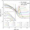 |
Fig. 1. Convective velocity as a function of age for different sets of models (DL models are drawn in solid lines and AMC models are shown in dotted lines). The curves referring to each stellar mass are drawn in a different colour according to the legend. Crosses (×) show the ZAMS ages for each mass model. The inset shows in detail the temporal evolution of vc during the beginning of the pre-MS phase. |
Values of vc decrease during early phases of the pre-MS, increase after the formation of the radiative core, and remain nearly constant during the MS; the higher the stellar mass, the higher the convective velocity. In the initial part of the pre-MS (3 ≲ log(t/yr)≲6), vc is slightly lower for models simulating DL than for AMC models, while during the MS, models simulating DL yield higher convective velocities. This change in the vc behaviour happens around 1 Myr, when AMC models become faster rotators than DL models.
The vc behaviour can be understood by means of an extension of the mass-lowering effect (Sackmann 1970), which states that rotating stars mimic non-rotating stars with smaller masses. Here, we are extending the mass-lowering effect to stars with different rotation rates, in which stars with higher rotation rates mimic non-rotating stars with even lower masses than stars with lower rotation rates do. The fractional mass of the radiative core of each stellar mass for AMC and DL models, shown in Fig. 2, seem to corroborate our ideas. AMC models produce smaller fractional radiative core masses than DL models, as if they were models with smaller masses.
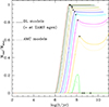 |
Fig. 2. Fractional mass of the radiative core for DL and AMC models. Symbols and colours are the same as in Fig. 1. |
A consequence from the behaviour seen in Fig. 2 is that including disk-locking in the models results in weaker effects of rotation in the MS. During the disk-locking phase, stars contract keeping their angular velocities constant until the dissipation of the disk (∼3 Myr), when they start spinning-up conserving angular momentum, resulting in slower rotation rates in the MS, as compared with AMC models, that evolve without any locking. So, the faster the rotation, the stronger the mass-lowering effect and the slower the convective velocities. In the MS, the differences in vc are higher for more massive stars, except for the 0.1 M⊙ model, whose difference in convective velocity obtained by the two sets of models is comparable to that obtained by the 1.2 M⊙ model.
3.2. Global convective turnover times calculations
The global (or non-local) convective turnover time, τg, is defined as
 (2)
(2)
where Rstar is the stellar radius and Rb is the radial position of the base of the convective zone, the same as that of the tachocline for partially convective stars; Rb = 0 (stellar centre) for fully convective stars. According to Kim & Demarque (1996), τg is the characteristic timescale of the convective overturn. It can be used to depict convection features of the whole stellar convective region at each evolutionary stage, representing an average convective timescale over the entire convective zone. In the absence of a suitable prescription to calculate local convective turnover times of fully convective stars, τg is used to evaluate their Rossby numbers instead of τc (Irving et al. 2023). Fig. 3 shows the global convective turnover times produced by AMC and DL models as a function of age and mass. The behaviour of τg is a consequence of its definition (Eq. (2)), which depends directly on the actual extension of the convective zone (rconv), but inversely on the convective velocity. For a star of a given mass and age, various combinations of these two effects can yield higher or lower τg, depending on which effect is dominant.
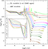 |
Fig. 3. Global convective turnover time as a function of age and stellar mass for different sets of models. The inset shows in detail the time evolution of τg during the beginning of the pre-MS phase. Colours and symbols are the same as in Fig. 1. |
The behaviour of vc was already discussed in Section 3.1 and before getting into the analysis of τg, we describe the behaviour of the extension of the convective zone in absolute terms. Fig. 4 shows how rconv varies with mass, age and model used. In the pre-MS (to the left of the crosses defining the ZAMS), rconv increases with mass and decreases with the stellar age. In the very early phase of evolution (up to 103 to 104 years, depending on the stellar mass), rconv produced by AMC models is smaller than that yielded by DL models. After that age (and up to the ZAMS), the behaviour of rconv is reversed. In the MS (to the right of the crosses in Fig. 4), rconv shows small changes with age for a given mass, but varies in a more complex way with mass. It sharply increases with mass from 0.1 to 0.3 M⊙, decreases abruptly from 0.3 to 0.4 M⊙ (because the star develops a radiative core), then gradually increases from 0.4 to 1.0 M⊙, reaches a local maximum (smaller than that for 0.3 M⊙), and decreases again from 1.0 to 1.2 M⊙. According to the model used, DL models produce rconv larger than AMC models for MS stars with M ≤ 0.3 M⊙, while for MS stars with M > 0.3 M⊙ AMC models yield larger rconv than DL models do.
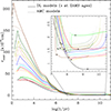 |
Fig. 4. Extension of the convective envelope in absolute terms (from the base to the top) as a function of mass and age for DL and AMC models. The inset shows in detail the time evolution of rconv during the MS phase. Symbols and colours are the same as in Fig. 1. |
As well as Landin et al. (2023), we notice that the time evolution of τg, showed in Fig. 3, is different for fully and partially convective stars. For very low-mass stars (M ≤ 0.3 M⊙), one can see only small variations (a factor of 3.5) on global convective turnover times, while variations reach almost four orders of magnitude for stars with M > 0.3 M⊙.
For M ≤ 0.3 M⊙, the global convective turnover time does not vary significantly with age during the pre-MS and MS phases of evolution (less than one order of magnitude). In the beginning of the pre-MS (t ≲ 106 years), τg decreases with increasing mass, but in the MS the opposite trend is observed. This is due to the behaviour of vc and rconv (Figs. 1 and 4, respectively), which essentially increase with mass for all ages, so that the former contributes to decrease τg and the latter contributes to increase it. In the pre-MS, the dominant effect on τg is that of vc and in the MS the dominant effect is that provided by rconv.
For M > 0.3 M⊙, τg values do not change significantly with age for a given mass in the beginning of the pre-MS phase, in which stars are fully convective, then decrease when the radiative core is formed, and remain roughly constant during the MS phase. In the pre-MS, the higher the stellar mass the higher τg. As can be seen in Figs. 1 and 4, both vc and rconv basically increase with mass for all ages, such that the effect of vc leads to a decrease in τg, while rconv causes an increase in τg. In this initial evolutionary phase, the influence of rconv dominates that of vc in the behaviour of τg. In the MS, τg increases with decreasing mass. Across this entire mass range, vc increases with the stellar mass, contributing to decrease τg, while rconv has a more complex behaviour. In the mass ranges 0.3–0.4 M⊙ and 1.0–1.2 M⊙, rconv decreases with mass, reinforcing the effect of vc and contributing to reduce τg with mass, and in the range 0.4–1.0 M⊙, rconv increases with mass, opposing the effect of vc and contributing to increase τg with mass. The combination of these two effects results in the prevalence of vc in the behaviour of τg, making τg decreases with increasing mass.
In our calculated models, the behaviour of τg depends on the stellar mass. In the beginning of the pre-MS, the global convective turnover time is practically model independent. For M ≥ 0.8 M⊙, AMC models generate τg slightly longer than DL models, while for M < 0.7 M⊙, the opposite trend is observed. It seems that 0.7 M⊙ is a transition mass for this behaviour. In the MS, τg is shorter for DL models in comparison with AMC ones (τg, DL < τg, AMC), except for 0.2 and 0.3 M⊙. For M ≤ 0.3 M⊙, DL models produce larger convective zones than AMC models (rconv, DL > rconv, AMC), favouring τg, DL > τg, AMC, while the convective velocities yielded by DL models are larger than those produced by AMC models (vc,DL > vc,AMC), favouring τg, DL < τg, AMC. The interplay between these two effects is dominated by the size of the convective zone for 0.2 and 0.3 M⊙ (producing τg, DL > τg, AMC) and by the convective velocity for 0.1 M⊙ (yielding τg, DL < τg, AMC). Among the fully convective models (M ≤ 0.3 M⊙), one sees that the behaviour of DL and AMC models for 0.1 M⊙ is the opposite of those of 0.2 and 0.3 M⊙. This can be explained by the fact that vc (Fig. 1) produced by AMC models for 0.2 and 0.3 M⊙ are only slightly lower than those yielded by DL models while, for 0.1 M⊙, AMC models produce vc noticeably lower than DL models do. Analyses with finer mass grid models (0.085, 0.09, 0.11, 0.12, 0.13, 0.14, and 0.15 M⊙, not shown here) reveal that such a switch in τg behaviour occurs between 0.10 and 0.11 M⊙ and τg, DL continues smaller than τg, AMC for masses smaller than 0.10 M⊙ (see the following quantitative comparisons between DL and AMC values of τg at 10 Gyr: τg, DL/τg, AMC is 1.0251 for 0.12 M⊙, 1.0041 for 0.11 M⊙, 0.8765 for 0.10 M⊙, 0.8423 for 0.09 M⊙, and 0.9102 for 0.085 M⊙). As the additional AMC models also present convergence issues when adopting the central values of JKaw as Jin, we used smaller input values which vary from 0.987 JKaw for 0.085 M⊙ to 0.997 JKaw for 0.15 M⊙. According to our AMC models, τg decreases with increasing Jin. If it were not for some convergence difficulties and had we used Jin = JKaw for models with M ≤ 0.15 M⊙, we would have obtained τg, DL even smaller than τg, AMC, making the change in τg behaviour near 0.1 M⊙ even more pronounced. For M > 0.3 M⊙, the behaviour of τg depending on the model used can be explained in a much simpler way, given that rconv, DL < rconv, AMC and vc,DL > vc,AMC, both effects contribute to generate τg, DL < τg, AMC.
3.3. Local convective turnover times calculations
The characteristic convective overturn timescale used to compute Rossby numbers is the local convective turnover time, which differs from τg only by a factor. It is defined as τc = ℓ/vc and is evaluated in deep regions of the convective envelope, where dynamo generation of magnetic fields is supposed to take place (Kim & Demarque 1996). Fig. 5 shows local convective turnover times as a function of age and mass. For partially convective configurations, τc is calculated at the standard location, r, one-half of a mixing length above the base of the convective zone. For fully convective configurations (whose r are larger than the stellar radii), τc is calculated at an alternative place related to Hp, as described in Landin et al. (2023). τc behaves roughly as τg, both as a function of age and as a function of mass, with some differences in the low mass regime and in the range of 1–11 Myr, when τc produced by models with M ≤ 0.3 M⊙ become smaller than those for 0.4 M⊙ models, as opposed to what happens regarding τg. This is probably due to the method used to calculate τc for fully convective stars, based on different linear fits for different age intervals and excluding higher masses because they deviate more from the linear behaviour; see Landin et al. (2023) for more details. In the pre-MS, τc is approximately constant and does not show a strong dependence with modelling (differences are around 1%). AMC models tend to produce higher τc for higher masses (M > 0.7 M⊙) and DL models tend to yield higher τc for smaller masses (M < 0.6 M⊙). As the stellar age increases, the cumulative effects of evolving with a higher angular velocity reflect in the convective properties of the stars and the differences in τc produced by the two sets of models reach 8–10% for ages greater than 100 Myr. Stars with M ≥ 1 M⊙ present the highest differences. In the MS, values of τc generated with models simulating the DL mechanism are shorter than those obtained with AMC models, except for 0.2 and 0.3 M ⊙, repeating the previously described behaviour of τg.
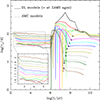 |
Fig. 5. Local convective turnover time as a function of age and stellar mass for different sets of models. Symbols and colours have the same meanings as in Fig. 1. The inset shows in detail the time evolution of τc during the beginning of the pre-MS phase. |
The top panel of Figure 6 shows the local convective turnover time as a function of age and mass produced by DL models with different locking periods (Plock ∼ 8 days and Plock = 400 days, keeping the same Tdisk = 3 Myr). For clarity, we show plots only for four stellar mass models, 0.1, 0.4, 0.7 and 1.0 M⊙. DL models with longer locking periods produce slightly longer values of local convective turnover times (except for the 1.0 M⊙ at the MS, for which τc is almost model independent). The reason is that DL models with Plock = 400 days have larger mixing lengths and convective velocities than those with Plock = 8 days, that contribute to increase and decrease τc, respectively, and the dependence on ℓ dominates over that on vc. The bottom panel of Fig. 6 shows the local convective turnover time as a function of age and mass produced by DL models with different disk lifetimes (Tdisk = 1 and 3 Myr, keeping the same Plock ∼ 8 days). We again show plots only for four stellar mass models, 0.1, 0.4, 0.7 and 1.0 M⊙. For all evolutionary phases and masses, DL models with Tdisk = 1 Myr yield slightly longer τc than DL models with Tdisk = 3 Myr, because, while ℓ is almost independent on Tdisk, DL models with Tdisk = 1 Myr produce convective velocities slightly lower than those with Tdisk = 3 Myr, since τc ∝ 1/vc.
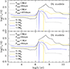 |
Fig. 6. Local convective turnover time as a function of age and mass for DL models with different locking periods (top panel) and different disk lifetimes (bottom panel). Colours are the same as in Fig. 1. |
τg and τc are quantities that cannot be directly observed and the best way to estimate them is through stellar evolutionary models. They are extensively used to determine Rossby numbers of stars operating different types of dynamos. τc is employed in stars that have tachocline-based dynamos and, when there is no suitable prescription to obtain it for stars that have no tachocline and harbour distributed dynamos, τg is used. τg and τc are mainly determined by the stellar mass, but non-standard physical ingredients, like the rotation rate, the way angular momentum evolves, and disk-locking parameters, have secondary effects, as discussed in Sections 3.2 and 3.3.
After investigating the local convective turnover time behaviour as a function of age obtained by models with different DL parameters, Fig. 7 shows how τc and τg vary with the effective temperature at the ZAMS. This plot is of particular interest due to its adequacy in obtaining the Rossby number using a quantity obtainable through observational data. As both global and local convective turnover times practically do not change during the main sequence (see Figs. 3 and 5), their ZAMS values are representative for their entire main sequence. The effective temperatures at the ZAMS, the ZAMS ages themselves, and both global and local convective turnover times are slightly model dependent, in such a way that the differences increase with the decreasing effective temperatures (i.e. in the lower-mass regime).
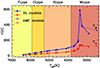 |
Fig. 7. Similarly to Fig. 13 of Irving et al. (2023), we show local (red) and global (blue) convective turnover times for AMC (dotted lines with open squares) and DL (solid lines with full squares) models as a function of effective temperature at the ZAMS. We use an updated version of Pecaut & Mamajek (2013) effective temperature-spectral type relation, https://www.pas.rochester.edu/~emamajek/EEM_dwarf_UBVIJHK_colors_Teff.txt |
4. Comparison with observations
In order to test our theoretical convective turnover times, we used them to calculate Ro for 73 late-F, G, K and M dwarf stars (both pre-MS and MS from the sample of Vidotto et al. 2014) and to investigate the magnetic activity-rotation relationship. The sample is formed by solar-like stars [MS stars with masses and ages in the ranges 0.66 ≤ M/M⊙ ≤ 1.34 and 260 ≤ t(Myr) ≤ 8700, including the Sun itself], young suns [non-accreting pre-MS and young MS stars with masses and ages in the ranges 0.54 ≤ M/M⊙ ≤ 1.50 and 10 ≤ t(Myr)≤130], hot-Jupiter (h−J) hosts [MS stars with masses and ages in the ranges 0.79 ≤ M/M⊙ ≤ 1.34 and 600 ≤ t(Myr) ≤ 5000 that host planets as massive as Jupiter in very close orbits], M dwarfs [MS and non-accreting pre-MS stars with masses and ages in the ranges 0.10 ≤ M/M⊙≤0.75 and 21 ≤ t(Myr) ≤ 1200], and Classical T Tauri stars [accreting pre-MS stars with masses and ages in the ranges 0.65 ≤ M/M⊙ ≤ 2.00 and 1.4 ≤ t(Myr) ≤ 17]. Vidotto et al. (2014) separated their sample in these subsamples in order to investigate whether the stars in these subgroups showed any specific behaviour in the rotation-magnetic activity diagram. They did not find any particular trend for any of these subgroups other than those already known: fully convective stars tend to occupy the saturated region and partially convective ones occupy both regions. Values of mass, age (except for 12 M dwarfs and one T Tauri star), Prot, LX/Lbol, and ⟨|BV|⟩ were taken from Vidotto et al. (2014). The ages of the 12 M dwarfs without age estimates in Vidotto et al. (2014) were determined using our evolution models. The age of the T Tauri star CV Cha used by Vidotto et al. (2014) is 4.8 Myr, taken from the value of (5 ± 1) Myr determined by Hussain et al. (2009). By using this age and our local convective turnover time, the Rossby number of CV Cha is too high, diverging considerably from the typical values of other T Tauri stars of our sample (as can be seen as open green triangles in Figs. 8 and 9). We, then, took the inferior limit of the value published by Hussain et al. (2009), i.e. 4 Myr, as the age of CV Cha, which coincides, within the errors, with the value of (4.2 ± 0.3) Myr found using the ATON code. Next, given the stellar mass and age of each object, their Rossby numbers were obtained using the observed rotation periods from Vidotto et al. (2014) and the local convective turnover times produced by our DL and AMC models. The rotation-activity relation of our sample was analysed using two different indicators of magnetic activity: LX/Lbol and ⟨|BV|⟩. Before getting into the details of our calculations, we outline the general procedure used for both indicators:
-
We initially fit the distribution of stars in the rotation-activity diagram with the following two-part, power-law functions,
 (3)
(3) (4)
(4)where β is the power-law slope in a log-log plot for the unsaturated region and C is a constant. Given an initial guess value for Rosat, we determine either (LX/Lbol)sat or ⟨|BV|⟩sat, which are respectively the average values of LX/Lbol and ⟨|BV|⟩ for Ro ≤ Rosat. For Ro > Rosat, we fit the data by using an iterative linear regression fit in a log-log scale, keeping the constant coefficient fixed, so that the values of either LX/Lbol or ⟨|BV|⟩ at Rosat are respectively equal to (LX/Lbol)sat and ⟨|BV|⟩sat.
-
Next we follow Vidotto et al. (2014) and Jackson & Jeffries (2010) and fix the saturation Rossby number at its canonical value, Rosat = 0.1, first estimated by Pizzolato et al. (2003), and determine the best parameters that fit the data to Eqs. (3) or (4), i.e. β and (LX/Lbol)sat or ⟨|BV|⟩sat. This approach is referred to as “Method A”.
-
A second estimate of Rosat is obtained by using an iterative least squares method to find the value at which the standard deviation of the data reaches its minimum and, again, we get the corresponding values of (LX/Lbol)sat, ⟨|BV|⟩sat, and the best fitting slopes for the unsaturated region for both LX/Lbol and ⟨|BV|⟩ indicators. This approach is referred to as “Method B”.
-
A third and last estimate for Rosat is made by choosing the value for which a least squares fit to the data results in the best fit to the Sun at its maximum, average and/or minimum activity levels. Then, as previously, we obtain the corresponding values of (LX/Lbol)sat, ⟨|BV|⟩sat, and β. This approach is referred to as “Method C”.
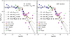 |
Fig. 8. log(LX/Lbol) × log(Ro) for stars in the sample of Vidotto et al. (2014). In the left panel, τc values, which enter in Ro calculations, were obtained from DL models with Plock ∼ 8 days and Tdisk = 3 Myr. In the right panel, τc values were obtained from AMC models. Solar-like stars are shown as |


4.1. Using LX/Lbol as the magnetic activity indicator
Among the 73 stars in the sample of Vidotto et al. (2014), 11 have no fractional X-ray luminosity determination, reducing our sample to 62 stars in the analysis involving LX/Lbol as the magnetic activity indicator. We initially analyse the rotation-activity relationship of our sample by using LX/Lbol and Ro calculated with τc from DL models with Plock ∼ 8 days and Tdisk = 3 Myr. The left panel of Fig. 8 shows our star sample in the log(LX/Lbol)×log(Ro) plane, with different symbols and colours.
For Rosat = 0.1 (Method A), the best fitting slope for the unsaturated part of the relation (see Eq. (3)) is found to be β = −1.9 ± 0.2, with the Pearson correlation coefficient |ρ| = 0.66, and the saturation level is estimated to be log(LX/Lbol)sat = −3.26 ± 0.06 (dotted curve in the left panel of Fig. 8). These values are consistent with those found by, e.g. Wright et al. (2011, 2018). For Rosat obtained through Method B, we find Rosat = 0.042 ± 0.003, β = −1.3 ± 0.2 (with |ρ| = 0.80), and log(LX/Lbol)sat = −3.20 ± 0.07 (dashed curve in the left panel of Fig. 8). Although the log(LX/Lbol)sat obtained in the last case is consistent with those found in the literature, the values of β and Rosat are considerably higher and smaller, respectively. Notice that none of these methods fits the minimum or the maximum Sun (black circles). By applying Method C, we could not fit the minimum Sun, while the Sun’s position in its average level of activity (the average Sun) was only achieved with fitting parameters in disagreement with the literature. However, we could fit the maximum Sun, finding Rosat = 0.19, β = −2.7 ± 0.4 (with |ρ| = 0.61), and log(LX/Lbol)sat = −3.28 ± 0.05 (solid black line in the left panel of Fig. 8).
These values are consistent with those found in the literature, with the value of β matching that of Wright et al. (2018) within the errors and coinciding with that of Wright et al. (2011). The value of Rosat is slightly larger than those of Wright et al. (2011, 2018) and log(LX/Lbol)sat is moderately smaller than (but still consistent with) those obtained by both mentioned works. For these reasons, and also because this fit reproduces the maximum Sun’s position in the rotation-activity diagram with consistent parameters, we consider it the best fit using DL models. For comparison, the best fit found by Wright et al. (2011), obtained using another sample of stars, is also shown in the left panel of Fig. 8. Table 2 shows the fit parameters found in this subsection (using τc provided by DL models) and those found by Wright et al. (2011) and Wright et al. (2018).
Fit parameters of the rotation-magnetic activity relationship in this work, W11 (Wright et al. 2011), W18 (Wright et al. 2018), and G24 (Galvão et al. 2024).
Using values of τc calculated with AMC models, we obtain the Rossby numbers of all stars in our sample displayed in the rotation-activity diagram, shown in the right panel of Fig. 8. As for the DL case, we fit the AMC data with three values of Rosat. For Rosat = 0.1 (Method A), we find a power index β = −2.0 ± 0.2 (with ρ = 0.69) and a saturation level of log(LX/Lbol)sat = −3.27 ± 0.06 (dotted curve in the right panel of Fig. 8). These values are consistent with those found in the literature, but log(LX/Lbol)sat is slightly low. Then, by using Method B, we find Rosat = 0.049 ± 0.006, β = −1.5 ± 0.2 (with |ρ| = 0.81), and log(LX/Lbol)sat = −3.20 ± 0.07 (dashed curve in the right panel of Fig. 8). These values of Rosat and β are compatible with those found in the literature, despite being marginally lower and higher, respectively, while the saturated value of LX/Lbol matches the one found by Wright et al. (2011) within the uncertainties. Nearly identical parameters are obtained for this sample by Galvão et al. (2024), who used τc determined with evolutionary tracks from the ATON code (similar to AMC models) and a Markov Chain Monte Carlo (MCMC) fitting method. Again, as can be seen from the right panel of Fig. 8, the dotted and dashed curves do not fit the Sun. Using Method C, we obtain a saturation Rossby number of Rosat = 0.14. This method fits the maximum Sun, provides log(LX/Lbol)sat = −3.28± 0.05 and β = −2.4 ± 0.3 (with |ρ| = 0.66), and is shown as a solid curve in the right panel of Fig. 8. The value of Rosat agrees with those found by Wright et al. (2011) and Wright et al. (2018) and is moderately larger than that found by Landin et al. (2023), while the value of β agrees, within the uncertainties, with those found by Wright et al. (2011), Wright et al. (2018), and Landin et al. (2023), that used much larger samples of stars (824 stars for the former work and 847 stars for the latter ones). Likewise, this value of log(LX/Lbol)sat is consistent with those found by these authors, although a little smaller. As in the case of DL models, this method cannot fit the minimum Sun and fits the average Sun with conflicting parameters. For the same reasons discussed in the analysis of the rotation-activity diagram with τc obtained by DL models, the parameters that fit the maximum Sun seem to be the more reliable ones when AMC models are used to calculate τc and they are shown in Table 2, together with the other AMC fits obtained in this subsection. For comparison purposes, the best fit found by Wright et al. (2011) using another sample of stars is also shown in the right panel of Fig. 8.
The values obtained for β and log(LX/Lbol)sat with τc calculated by AMC models agree, within the errors, with the corresponding values obtained by DL models. Regarding the fits obtained with Methods A and B, the β values are slightly smaller for AMC models and the opposite situation is observed by the fits which reproduce the Sun’s position in its maximum activity level (Method C). For both sets of models, we consider that the fits which better predict the solar magnetic activity level are the best ones. Besides fitting the Sun, they present Rosat and β in accordance with what was found in the works of Wright et al. (2011, 2018).
As we can see in Fig. 5, τc produced by AMC models are higher than those generated by DL models for most stellar ages, implying in smaller Rossby numbers. In fact, the average value of Rossby numbers obtained with DL models, ⟨RoDL⟩, is 21% higher than that obtained with AMC models, ⟨RoAMC⟩, which causes a slight global shift of the star distribution to the left in the rotation-activity diagram. However, this does not translate into a lower saturation Rossby number in our least squares fit, due to the high dispersion of the data. The fact that ⟨RoDL⟩ is larger than ⟨RoAMC⟩ indicates that stars that had experienced (or are experiencing) a locking phase present higher Rossby numbers and then, lower dynamo numbers, which means lower efficiency in the dynamo generation process.
It is already known that internal redistribution of angular momentum and angular momentum loss by stellar magnetised winds can significantly affect the stellar angular momentum evolution. As for the moment, we cannot consider yet these effects in our results because the ATON code version that takes the disk-locking mechanism into account is currently implemented only for rotational scheme 1 (solid body rotation), while the effects related to angular momentum variation are implemented only for rotational scheme 3 (differential rotation in radiative regions and solid body rotation in convective zones). At 100 Myr, τc obtained for 0.4 and 1.0 M⊙ models considering redistribution of angular momentum and angular momentum loss by winds is around 94% of the value obtained when considering solid body rotation with no effects related to angular momentum variability. As far as we can foresee, our DL and AMC models would be affected roughly the same way by the inclusion of such effects, keeping invariable the relative differences between our results obtained with the two sets of models. Including these effects would cause DL and AMC models to produce τc values a few percent lower. Consequently, the Rossby numbers obtained for the stars of our sample would be slightly higher (shifting the star distributions in both panels of Fig. 8 to the right), which would probably slightly increase Rosat. Nevertheless, we plan to improve the ATON code in order to fully account for these effects.
4.2. Using ⟨|BV|⟩ as the magnetic activity indicator
The sample of Vidotto et al. (2014) consists of 104 magnetic maps of 73 stars, constructed with observations made at multiple epochs, resulting in 102 pairs of measurements of unsigned average large-scale surface magnetic fields and rotation periods, which allow us to use ⟨|BV|⟩ as the magnetic activity indicator in the analysis of the rotation-activity relation of our sample. Initially, we used Rossby numbers calculated by DL models with Plock ∼ 8 days and Tdisk = 3 Myr. In the left panel of Fig. 9, we show the stars of our sample in the log(⟨|BV|⟩) × log(Ro) plane with the same symbols and colours used in Fig. 8.
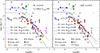 |
Fig. 9. log(⟨|BV|⟩) × log(Ro) for stars in the sample of Vidotto et al. (2014). In the left panel, the τc values, which enter in Ro calculations, were obtained from DL models with Plock ∼ 8 days and Tdisk = 3 Myr. In the right panel, τc values were obtained from AMC models. Symbols are the same as in Fig. 8. |
The same general procedure used for the log(LX/Lbol) indicator is adopted and, for Rosat = 0.1 (Method A), we find β = −1.70 ± 0.15, as the best fitting slope for the unsaturated part of the relation (see Eq. (4)), with ρ = 0.66, and the saturation level of activity is found to be log(⟨|BV|⟩/G)sat = 2.28 ± 0.06 (dotted curve in the left panel of Fig. 9). The value of β is nearly in agreement with that of Vidotto et al. (2014) within the uncertainties. Our value of log(⟨|BV|⟩)sat is between the saturation value found by Vidotto et al. (2014) for the early M dwarfs (early-dM, M ≥ 0.4 M⊙, log(⟨|BV|⟩/G)sat = 1.7) and the value found for mid M dwarfs (mid-dM, 0.2 < M/M⊙ < 0.4, log(⟨|BV|⟩/G)sat = 2.6). These two saturation levels are shown as horizontal dot-dashed lines in both panels of Fig. 9. With Method B, we find Rosat = 0.033 ± 0.012, β = −0.98 ± 0.11 (with |ρ = 0.81|), and log(⟨|BV|⟩/G)sat = 2.25 ± 0.14 (dashed curve in the left panel of Fig. 9). These values of β and ⟨|BV|⟩sat are consistent with those found by Vidotto et al. (2014), but our β is slightly higher and our Rosat is considerably lower. According to See et al. (2019), who also find a Rosat smaller than Vidotto et al. (2014) but a little larger than this work, obtaining a smaller value of Rosat could be due to a number of reasons. They mention that a poorly constrained level of the saturation field strength and differences in the way to calculate the convective turnover times can affect the Rosat value. In addition, they emphasise that different activity indicators could saturate at different Rossby numbers. As can be seen in the left panel of Fig. 9, our fit obtained through Method B fits the Sun in its maximum level of activity, while our fit with Rosat = 0.1 (Method A) nearly fits the Sun in its minimum. Although Method B fitted the maximum Sun, we applied Method C and, with it, we were also able to reproduce the minimum and the average Sun, in addition to the maximum Sun, with plausible parameters, similar to those found by See et al. (2019) and Galvão et al. (2024). We decided to present only the parameters that fit the maximum Sun because this was the only level of solar activity that we were able to reproduce with Method C, employing the two magnetic activity indicators used in this work. For comparison, the best fit found by Vidotto et al. (2014) is also shown in the left panel of Fig. 9 as dot-dashed lines. Here, it is worth mentioning that our fit includes all T Tauri stars and the 12 M dwarfs without age estimates in Vidotto et al. (2014) but these stars did not enter in their fit. Table 3 shows the fit parameters found in this subsection (using τc provided by DL models) and those found by Vidotto et al. (2014) and See et al. (2019).
Fit parameters of the rotation-magnetic activity relation in this work, Vidotto et al. (2014), See et al. (2019), and Galvão et al. (2024).
Finally, we investigate the rotation-activity relationship of our sample by using our local convective turnover times obtained with AMC models to calculate the Rossby number of all stars. Our sample is displayed in the rotation-activity diagram shown in the right panel of Fig. 9 and the data were fit with the two-part power-law function expressed in Eq. (4). We again perform three fits to our data by imposing ⟨|BV|⟩ = ⟨|BV|⟩sat at Rosat. For Rosat = 0.1 (Method A), we find β = −1.72 ± 0.15 (with ρ = 0.68) and log(⟨|BV|⟩/G)sat = 2.20 ± 0.09 (dotted curve in the right panel of Fig. 9). This value of ⟨|BV|⟩sat is between the values proposed by Vidotto et al. (2014) and in agreement with that of See et al. (2019) within the uncertainties and this value of β is consistent with that published by both works. Next, we apply Method B and find Rosat = 0.036 ± 0.08, β = −1.13 ± 0.11 (with ρ = 0.80), and log(⟨|BV|⟩/G)sat = 2.30 ± 0.12 (dashed curve in the right panel of Fig. 9). Although this Rosat is considerably smaller than others found in the literature (except that of See et al. 2019), this value of β matches that of Vidotto et al. (2014) within the errors and nearly matches that of See et al. (2019). Furthermore, this value of ⟨|BV|⟩sat is consistent with those found by both works. Even by using a different fitting method (MCMC), Galvão et al. (2024) also found similar parameters as in our analysis. As one can see in the right panel of Fig. 9, the dotted curve nearly fits the minimum Sun and the dashed curve is close to the maximum Sun. So, our last fit aimed to get a better fit to the maximum Sun by means of Method C, resulting in Rosat = 0.025, which is considerably lower than the values found in the literature. This last fit also provides β = −0.96 ± 0.10 and log(⟨|BV|⟩/G)sat = 2.29 ± 0.15 (with |ρ| = 0.81, seen in solid line in the right panel of Fig. 9). These values are consistent with those found by Vidotto et al. (2014) and See et al. (2019), although the value of β is somewhat higher. With Method C, we can also fit both the minimum and the average Sun with consistent parameters. As in the previous analysis, the parameters that fit the Sun in the study of the rotation-activity relation using ⟨|BV|⟩ as an activity indicator and τc generated by AMC models (all shown in Table 3) are also considered the more reasonable ones. For comparison, the best fit found by Vidotto et al. (2014) is also shown in the right panel of Fig. 9 as dot-dashed lines. The values obtained for β and ⟨|BV|⟩sat with τc calculated by AMC models agree, within the errors, with those obtained by the corresponding fits with τc calculated by DL models.
As described in Section 4.1, the values of Rossby numbers obtained with τc produced by AMC models are lower than those generated by DL models and this manifests itself as a slight shift of the stars distribution to the left in the right panel of Fig. 9 relative to those in the same figure’s left panel. For this subsample, ⟨RoDL⟩ = 1.27 ⟨RoAMC⟩, what would again imply that stars which pass through a locking phase would have a smaller dynamo number and, consequently, would operate a less efficient dynamo. However, as in Section 4.1, Rosat, DL < Rosat, AMC, probably due to the high dispersion of the data. Lastly, the inclusion of redistribution of angular momentum and angular momentum loss by winds would affect the results obtained with DL and AMC models in a similar fashion, slightly increasing the stars Rossby numbers and moving the whole star distributions in both panels of Fig. 9 to the right, as discussed in the previous subsection.
5. Conclusions
We present new sets of pre-MS and MS evolutionary tracks considering the disk-locking mechanism and the conservation of angular momentum, including Rossby numbers, global and local convective turnover times in the mass range of 0.1–1.2 M⊙. We compare τg, τc, and vc produced by the two sets of models considering both evolutionary phases (pre-MS and MS). The differences are smaller in the early pre-MS (∼1%) and increase with stellar age, reaching 8–10% for ages greater than 100 Myr. The largest differences are found in stars with masses higher than or equal to 1 M⊙.
In the MS, models simulating the DL mechanism produce vc higher than models conserving angular momentum. The opposite behaviour is observed for τg and τc, except for 0.2 and 0.3 M⊙ models. More specifically, our results point out that stars which experience a locking phase reach the MS with smaller values of τc, larger Rossby numbers and smaller dynamo numbers, implying that their dynamo processes are less efficient in comparison with those stars that evolve conserving angular momentum since the beginning. By varying the initial angular momentum and the duration of the disk phase, we notice that the higher the initial velocity and Tdisk, the shorter τc. As the local convective turnover time is used to obtain the Rossby number, this suggests that properties of the disk phase of the star affect its Ro and its position in the rotation-activity diagram in the MS.
In the sequence, we use our theoretical convective turnover times to calculate Ro for 73 stars from the sample of Vidotto et al. (2014) to investigate the magnetic activity-rotation relationship. We plot the data in two versions of the rotation-activity diagram (LX/Lbol × Ro and ⟨|BV|⟩ × Ro) which show the typical saturated and unsaturated regimes. We fit the data with two-part power-law functions (Eqs. (3) and (4)) using three different methods. By considering the fit in the LX/Lbol × Ro diagram (with τc calculated by DL models) which reproduces the active Sun’s position (Method C), we find Rosat = 0.14, log(LX/Lbol)sat = −3.28±0.05, and the inclination of the unsaturated region is found to be β = −2.4 ± 0.3. By considering the best fit in the ⟨|BV|⟩ × Ro diagram which reproduces the Sun’s position in its maximum of activity (obtained with Method B), we find Rosat = 0.033 ± 0.012, log(⟨|BV|⟩/G)sat = 2.25 ± 0.15, and the power index of the unsaturated region is found to be β = −0.98 ± 0.11. These parameters are consistent to those usually found in the literature. We caution that these results are based on a relatively small sample, specially when it is compared to other similar works (for instance, Wright et al. 2011, 2018, and Newton et al. 2017). In addition, τc in Sections 4.1 and 4.2 were obtained assuming either that all stars had gone through a disk phase (with about the same locking period and during the same disk lifetime) or that they all evolved conserving angular momentum from the beginning. The most likely scenario is that some stars would have evolved with a very short disk-locking phase (Tdisk ≲ 105 yr) and can be considered as having evolved without a circumstellar disk since the start of their evolutions, while others would have spent some time in a locking phase with different locking periods and different disk lifetimes.
Finally, we speculate how internal redistribution of angular momentum and angular momentum loss by magnetised stellar winds would affect our results. We took such effects into account in 0.4 and 1.0 M⊙ models which rotate according to rotational scheme 3 and conserve angular momentum during all evolutionary phases and showed that it reduces τc in 6% at 100 Myr. We find no reason why these effects would affect DL models differently than AMC models (remembering that both were modelled with rigid body rotation). Therefore, the general behaviour we would expect for the stars in our sample in Section 4 is that they would have smaller τc, which would imply in a larger Ro and in a less efficient dynamo (ND ∝ Ro−2).
Data availability
The complete version of Table 1 is available at the CDS via anonymous ftp to cdsarc.cds.unistra.fr (130.79.128.5) or via https://cdsarc.cds.unistra.fr/viz-bin/cat/J/A+A/693/A68
For M ≥ 0.2 M⊙, the central values given by the Kawaler (1987) relation are used to obtain the initial angular momentum (Jin) of our models. Due to non-convergence reasons, we use a slightly smaller value of Jkaw as Jin for 0.1 M⊙, namely Jin = 7.943 × 1048 g cm2 s−1, which corresponds to a rotation period of ∼30 days and is within the error bars in Eq. (1).
Also due to non-convergence reasons, we use initial angular momenta smaller than those corresponding to 8 days for models with M ≥ 0.8 M⊙. The values used correspond to rotation periods of 8.5, 9.6, 10.6, 11.4, and 18.8 days for 0.8, 0.9, 1.0, 1.1, and 1.2 M⊙, respectively.
Acknowledgments
The authors thank Drs. Francesca D’Antona (INAF-OAR, Italy) and Italo Mazzitelli (in memoriam) for granting them full access to the ATON evolutionary code. They are also grateful to an anonymous referee for his/her many comments and suggestions that helped to improve this work. Financial support from the Brazilian agencies CAPES, CNPq and FAPEMIG is gratefully acknowledged.
References
- Alexander, D. R., & Ferguson, J. W. 1994, ApJ, 437, 879 [NASA ADS] [CrossRef] [Google Scholar]
- Allard, F., Hauschildt, P. H., & Schweitzer, A. 2000, ApJ, 539, 366 [NASA ADS] [CrossRef] [Google Scholar]
- Alphenaar, P., & van Leeuwen, F. 1957, Inf. Bull. Variable Stars, No. 1957 [Google Scholar]
- Asplund, M., Grevesse, N., Sauval, A. J., & Scott, P. 2009, ARA&A, 47, 481 [NASA ADS] [CrossRef] [Google Scholar]
- Attridge, J. M., & Herbst, W. 1992, ApJ, 398, 61 [Google Scholar]
- Böhm-Vitense, E. 1958, Z. Astroph., 46, 108 [Google Scholar]
- Choi, P. I., & Herbst, W. 1996, AJ, 111, 283 [NASA ADS] [CrossRef] [Google Scholar]
- Cieza, L., & Baliber, N. 2006, ApJ, 649, 862 [NASA ADS] [CrossRef] [Google Scholar]
- Donati, J.-F., & Landstreet, J. D. 2009, ARA&A, 47, 333 [NASA ADS] [CrossRef] [Google Scholar]
- Durney, B. R., De Young, D. S., & Roxburgh, I. W. 1993, Sol. Phys., 145, 207 [NASA ADS] [CrossRef] [Google Scholar]
- Flaccomio, E., Micela, G., & Sciortino, S. 2003, A&A, 402, 277 [NASA ADS] [CrossRef] [EDP Sciences] [Google Scholar]
- Galvão, L. J., Landin, N. R., & Alencar, S. H. P. 2024, Bol. Soc. Astronon. Brasil., 35, 160 [Google Scholar]
- Henderson, C. B., & Stassun, K. G. 2012, ApJ, 747, 51 [Google Scholar]
- Herbst, W., Bailer-Jones, C. A. L., Mundt, R., Meisenheimer, K., & Wackermann, R. 2002, A&A, 396, 513 [EDP Sciences] [Google Scholar]
- Hussain, G. A. J., Collier Cameron, A., Jardine, M. M., et al. 2009, MNRAS, 398, 189 [Google Scholar]
- Iglesias, C. A., & Rogers, F. J. 1993, ApJ, 412, 752 [Google Scholar]
- Irving, A. Z., Saar, H. S., Wargelin, B. J., & do Nascimento, J. D. 2023, ApJ, 949, 51 [NASA ADS] [CrossRef] [Google Scholar]
- Irwin, J., Hodgkin, S., Aigrain, S., et al. 2008, MNRAS, 384, 675 [CrossRef] [Google Scholar]
- Jackson, R. J., & Jeffries, R. D. 2010, MNRAS, 407, 465 [NASA ADS] [CrossRef] [Google Scholar]
- Kawaler, S. D. 1987, PASP, 99, 1322 [CrossRef] [Google Scholar]
- Kim, Y.-C., & Demarque, P. S. 1996, ApJ, 457, 340 [NASA ADS] [CrossRef] [Google Scholar]
- Lamm, M. H., Mundt, R., Bailer-Jones, C. A. L., & Herbst, W. 2005, A&A, 430, 1005 [NASA ADS] [CrossRef] [EDP Sciences] [Google Scholar]
- Landin, N. R., Ventura, P., D’Antona, F., Mendes, L. T. S., & Vaz, L. P. R. 2006, A&A, 456, 269 [NASA ADS] [CrossRef] [EDP Sciences] [Google Scholar]
- Landin, N. R., Mendes, L. T. S., & Vaz, L. P. R. 2010, A&A, 510, A46 [NASA ADS] [CrossRef] [EDP Sciences] [Google Scholar]
- Landin, N. R., Mendes, L. T. S., Vaz, L. P. R., & Alencar, S. H. P. 2016, A&A, 586, A96 [NASA ADS] [CrossRef] [EDP Sciences] [Google Scholar]
- Landin, N. R., Chaves, J. K. L., Souza, T. S. M., et al. 2021, The 20.5th Cambridge Workshop on Cool Stars, Stellar Systems, and the Sun (CS20.5), online at, http://coolstars20.cfa.harvard.edu/cs20half, 329 [Google Scholar]
- Landin, N. R., Mendes, L. T. S., Vaz, L. P. R., & Alencar, S. H. P. 2023, MNRAS, 519, 5304 [NASA ADS] [CrossRef] [Google Scholar]
- Mendes, L. T. S., D’Antona, F., & Mazzitelli, I. 1999, A&A, 341, 174 [NASA ADS] [Google Scholar]
- Mihalas, D., Dappen, W., & Hummer, D. G. 1988, ApJ, 331, 815 [NASA ADS] [CrossRef] [Google Scholar]
- Mohanty, S., & Basri, G. 2003, AJ, 583, 451 [NASA ADS] [Google Scholar]
- Monsch, K., Drake, J. J., Garraffo, C., Picogna, G., & Ercolano, B. 2023, ApJ, 959, 140 [NASA ADS] [CrossRef] [Google Scholar]
- Nelson, O. R. 2008, Ph.D. Thesis, Federal University of Rio Grande do Norte, Natal, Brazil [Google Scholar]
- Newton, E. R., Irwin, J., Charbonneau, D., et al. 2017, ApJ, 834, 85 [Google Scholar]
- Noyes, R. W., Hartmann, S. W., Baliunas, S., Duncan, D. K., & Vaughan, A. 1984, ApJ, 279, 763 [NASA ADS] [CrossRef] [Google Scholar]
- Parker, E. N. 1955, ApJ, 122, 293 [Google Scholar]
- Pecaut, M. J., & Mamajek, E. E. 2013, ApJS, 208, 9P [NASA ADS] [CrossRef] [Google Scholar]
- Pizzolato, N., Maggio, A., Micela, G., Sciortino, S., & Ventura, P. 2003, A&A, 397, 147 [NASA ADS] [CrossRef] [EDP Sciences] [Google Scholar]
- Preibisch, T., Kim, Y. C., Favata, F., et al. 2005, ApJ, 160, 401 [NASA ADS] [Google Scholar]
- Prosser, C. F., Shetrone, M. D., Dasgupta, A., et al. 1995, PASP, 107, 211 [NASA ADS] [CrossRef] [Google Scholar]
- Rogers, F. J., Swenson, F. J., & Iglesias, C. A. 1996, ApJ, 456, 902 [Google Scholar]
- Sackmann, I.-J. 1970, A&A, 8, 76 [NASA ADS] [Google Scholar]
- See, V., Matt, S. P., Folsom, C. P., et al. 2019, ApJ, 876, 118 [Google Scholar]
- Skumanich, A. 1972, ApJ, 171, 565 [Google Scholar]
- Spiegel, E. A., & Zahn, J.-P. 1992, A&A, 265, 106 [Google Scholar]
- Stauffer, J. R., & Hartmann, L. W. 1987, ApJ, 318, 337 [NASA ADS] [CrossRef] [Google Scholar]
- Stauffer, J. R., Hartmann, L. W., Prosser, C. F., et al. 1997, ApJ, 479, 776 [NASA ADS] [CrossRef] [Google Scholar]
- Thompson, M. J., Christensen-Dalsgaard, J., Miesch, M. S., & Toomre, J. 2003, ARA&A, 41, 599 [Google Scholar]
- Vidotto, A. A., Gregory, S. G., Jardine, M., et al. 2014, MNRAS, 441, 2361 [Google Scholar]
- Wright, N. J., & Drake, J. J. 2016, Nature, 535, 526 [Google Scholar]
- Wright, N. J., Drake, J. J., Mamajek, E. E., & Henry, W. 2011, ApJ, 743, 48 [NASA ADS] [CrossRef] [Google Scholar]
- Wright, N. J., Newton, E. R., Williams, P. K. G., Drake, J. J., & Yadav, R. K. 2018, MNRAS, 479, 2351 [Google Scholar]
All Tables
Evolutionary track for 1 M⊙ star (DL model with Plock ∼ 8 days and Tdisk = 3 Myr).
Fit parameters of the rotation-magnetic activity relationship in this work, W11 (Wright et al. 2011), W18 (Wright et al. 2018), and G24 (Galvão et al. 2024).
Fit parameters of the rotation-magnetic activity relation in this work, Vidotto et al. (2014), See et al. (2019), and Galvão et al. (2024).
All Figures
|
Fig. 1. Convective velocity as a function of age for different sets of models (DL models are drawn in solid lines and AMC models are shown in dotted lines). The curves referring to each stellar mass are drawn in a different colour according to the legend. Crosses (×) show the ZAMS ages for each mass model. The inset shows in detail the temporal evolution of vc during the beginning of the pre-MS phase. |
| In the text | |
|
Fig. 2. Fractional mass of the radiative core for DL and AMC models. Symbols and colours are the same as in Fig. 1. |
| In the text | |
|
Fig. 3. Global convective turnover time as a function of age and stellar mass for different sets of models. The inset shows in detail the time evolution of τg during the beginning of the pre-MS phase. Colours and symbols are the same as in Fig. 1. |
| In the text | |
|
Fig. 4. Extension of the convective envelope in absolute terms (from the base to the top) as a function of mass and age for DL and AMC models. The inset shows in detail the time evolution of rconv during the MS phase. Symbols and colours are the same as in Fig. 1. |
| In the text | |
|
Fig. 5. Local convective turnover time as a function of age and stellar mass for different sets of models. Symbols and colours have the same meanings as in Fig. 1. The inset shows in detail the time evolution of τc during the beginning of the pre-MS phase. |
| In the text | |
|
Fig. 6. Local convective turnover time as a function of age and mass for DL models with different locking periods (top panel) and different disk lifetimes (bottom panel). Colours are the same as in Fig. 1. |
| In the text | |
|
Fig. 7. Similarly to Fig. 13 of Irving et al. (2023), we show local (red) and global (blue) convective turnover times for AMC (dotted lines with open squares) and DL (solid lines with full squares) models as a function of effective temperature at the ZAMS. We use an updated version of Pecaut & Mamajek (2013) effective temperature-spectral type relation, https://www.pas.rochester.edu/~emamajek/EEM_dwarf_UBVIJHK_colors_Teff.txt |
| In the text | |
|
Fig. 8. log(LX/Lbol) × log(Ro) for stars in the sample of Vidotto et al. (2014). In the left panel, τc values, which enter in Ro calculations, were obtained from DL models with Plock ∼ 8 days and Tdisk = 3 Myr. In the right panel, τc values were obtained from AMC models. Solar-like stars are shown as |
| In the text | |
|
Fig. 9. log(⟨|BV|⟩) × log(Ro) for stars in the sample of Vidotto et al. (2014). In the left panel, the τc values, which enter in Ro calculations, were obtained from DL models with Plock ∼ 8 days and Tdisk = 3 Myr. In the right panel, τc values were obtained from AMC models. Symbols are the same as in Fig. 8. |
| In the text | |
Current usage metrics show cumulative count of Article Views (full-text article views including HTML views, PDF and ePub downloads, according to the available data) and Abstracts Views on Vision4Press platform.
Data correspond to usage on the plateform after 2015. The current usage metrics is available 48-96 hours after online publication and is updated daily on week days.
Initial download of the metrics may take a while.