| Issue |
A&A
Volume 693, January 2025
|
|
|---|---|---|
| Article Number | A39 | |
| Number of page(s) | 13 | |
| Section | Extragalactic astronomy | |
| DOI | https://doi.org/10.1051/0004-6361/202449525 | |
| Published online | 03 January 2025 | |
Study of late-time ultraviolet emission in core collapse supernovae and its implications for the peculiar transient AT2018cow
1
Department of Astrophysics/IMAPP, Radboud University Nijmegen, P.O. Box 9010 6500 GL Nijmegen, The Netherlands
2
SRON, Netherlands Institute for Space Research, Niels Bohrweg 4, 2333 CA Leiden, The Netherlands
3
Department of Physics, University of Warwick, Gibbet Hill Road, Coventry CV4 7AL, UK
4
School of Physics, University College Dublin, L.M.I. Main Building, Beech Hill Road, Dublin 4 D04 P7W1, Ireland
5
Institute of Space Sciences (ICE-CSIC), Campus UAB, Carrer de Can Magrans s/n, E-08193 Barcelona, Spain
6
Institut d’Estudis Espacials de Catalunya (IEEC), E-08034 Barcelona, Spain
7
Tuorla Observatory, Department of Physics and Astronomy, 20014 University of Turku, Vesilinnantie 5, Turku, Finland
8
Finnish Centre for Astronomy with ESO (FINCA), 20014 University of Turku, Vesilinnantie 5, Turku, Finland
⋆ Corresponding author; This email address is being protected from spambots. You need JavaScript enabled to view it.
Received:
7
February
2024
Accepted:
11
November
2024
Abstract
Context. Over time, core-collapse supernova (CCSN) spectra become redder due to dust formation and cooling of the SN ejecta. An ultraviolet (UV) detection of a CCSN at late times will thus indicate an additional physical process, such as an interaction between the SN ejecta and the circumstellar material, or viewing down to the central engine of the explosion. Both of these models have been proposed to explain the peculiar transient AT2018cow, a luminous fast blue optical transient detected in the UV two to four years after the event, with only marginal fading over this time period.
Aims. To identify whether the late-time UV detection of AT2018cow could indicate that it is a CCSN, we investigate whether CCSNe are detectable in the UV between two and five years after the explosion. We determine how common late-time UV emission in CCSNe is and compare those CCSNe detected in the UV to the peculiar transient AT2018cow.
Methods. We used a sample of 51 nearby (z < 0.065) CCSNe observed with the Hubble Space Telescope within two to five years of discovery. We measured their brightness or determined an upper limit on the emission through an artificial star experiment in cases of no detection.
Results. For two CCSNe, we detected a point source within the uncertainty region of the SN position. Both have a low chance alignment probability with bright objects within their host galaxies. Therefore, they are likely to be related to their SNe, which are both known to be interacting SNe.
Conclusions. Comparing the absolute UV magnitude of AT2018cow at late times to the absolute UV magnitudes of the two potential SN detections, there is no evidence that a late-time UV detection of AT2018cow is atypical for interacting SNe. However, when limiting the sample to CCSNe closer than AT2018cow, we see that it is brighter than the upper limits on most CCSN non-detections. Combined with a very small late time photospheric radius of AT2018cow, this leads us to conclude that the late-time UV detection of AT2018cow was not driven by interaction. Instead, it suggests that we are possibly viewing the inner region of the explosion that is perhaps due to the long-lived presence of an accretion disc. Such properties are naturally expected in tidal disruption models and are less straightforward (though not impossible) in SN scenarios.
Key words: stars: massive / stars: individual: AT2018cow / supernovae: general / supernovae: individual: AT2018cow / ultraviolet: stars
© The Authors 2024
 Open Access article, published by EDP Sciences, under the terms of the Creative Commons Attribution License (https://creativecommons.org/licenses/by/4.0), which permits unrestricted use, distribution, and reproduction in any medium, provided the original work is properly cited.
This article is published in open access under the Subscribe to Open model. This email address is being protected from spambots. You need JavaScript enabled to view it. to support open access publication.
1. Introduction
Supernovae (SNe) are the explosive endpoints massive stars. With a steep increase in the number of telescopes built specifically to detect transients such as Zwicky Transient Facility (ZTF; Bellm et al. 2019), All-Sky Automated Survey for Supernovae (ASAS-SN; Shappee et al. 2014), Asteroid Terrestrial-Impact Last Alert System (ATLAS; Tonry 2011), and Gravitational-wave Optical Transient Observer (GOTO; Gompertz et al. 2020; Steeghs et al. 2022), the number of detected SNe has increased significantly. Over the next decade, the increase in sample size will accelerate with the commissioning of the Black hole Gravitational-wave ElectroMagnetic counterpart array (BlackGEM; Bloemen et al. 2016) and the Vera Rubin Observatory (Ivezić et al. 2019).
There are multiple types of SNe, observationally classified predominantly by the absence or presence of hydrogen in the explosion spectra, Type I and Type II SNe, respectively (Minkowski 1941). Within Type I SNe there are multiple sub-types, corresponding to different explosion mechanisms and progenitors. Type Ia SNe are caused by a thermonuclear explosion of a white dwarf (Nomoto et al. 1984; Woosley & Weaver 1986, and references therein). Their explosion spectra show strong silicon absorption features (e.g. Maguire 2017). Type Ib (Elias et al. 1985) and Ic (Wheeler & Harkness 1986) are core collapse SNe (CCSNe), which originate from massive stars (M > 8 M⊙, see Smartt 2009 for a review) that do and do not show helium features in their spectra, respectively. Stars can lose their hydrogen (and helium) envelopes through, for instance, mass transfer due to binary interactions (Podsiadlowski et al. 1992; Eldridge et al. 2008) and/or stellar winds (Vink et al. 2001; Crowther 2007). Additionally, Type Ic SN spectra can display very broad lines, known as Ic-BL (Modjaz et al. 2016; Sahu et al. 2018), or narrow emission lines (Type Icn; Fraser et al. 2021; Gal-Yam et al. 2022; Perley et al. 2022). Type Ib SN spectra occasionally have narrow lines (Type Ibn; Pastorello et al. 2007).
Type II SNe are also CCSNe, however, as mentioned before, their spectra contain hydrogen. The classes of CCSNe are also sub-divided based on their light curves, besides being classified based on spectral properties. Type II SNe are split into Type IIb, which have helium-rich spectra (Woosley et al. 1987), and IIn, which show narrow emission lines in their spectra (Schlegel 1990), as well as IIL, which show a linear decay in magnitude in their light curves, and IIP, which show a plateau of approximately constant brightness in their light curves (Barbon et al. 1979; Doggett & Branch 1985). In this paper, we focus on Type II CCSNe.
Besides removing (some of) the hydrogen and/or helium envelope, mass loss in massive stars can lead to a dense circumstellar medium (CSM) around a star. When the SN ejecta interact with this CSM, narrow emission lines will appear in the spectrum, creating Type In or IIn SNe (as noted above). Mass loss in massive stars can arise through different mechanisms. Besides stellar winds and binary interactions, eruptions can release material from the star (e.g. Smith & Arnett 2014; Yoshida et al. 2021). The shape and speed of the CSM combined with the speed and energy of the SN ejecta determines the (late-time) evolution of the light curve and spectra of interacting SNe (e.g. Dessart et al. 2015; Ercolino et al. 2024). We also refer to Dessart (2024) for a review of interacting SNe. Dessart et al. (2023) showed that for typical red supergiant (RSG) parameters, CSM interaction would predominantly cause extra brightening in the ultraviolet (UV), but not as much in the optical and infrared (IR). It is therefore most beneficial to study SNe in the UV to constrain the CSM interaction properties.
The classification of SN type is based on observational properties, which means it is not always clear-cut. It can change over time as emission lines appear and disappear due to, for instance, interactions with the CSM. For example, Dong et al. (2024) showed that the classification of SN2022cvr changes from IIb to Ib over time. There are also works that have demonstrated that Type IIP and Type IIL SNe are not two distinct types, but rather a continuum of slopes in the plateau, attributed to the various amounts of hydrogen that are present (e.g. Anderson et al. 2014; Sanders et al. 2015; Galbany et al. 2016a; Hiramatsu et al. 2021).
With the increase in survey cadence and depth of transient surveys, an increase in the number of peculiar transients has also occurred. For example, luminous fast blue optical transients (LFBOTs; e.g. Inserra 2019; Metzger 2022) can spectroscopically resemble SNe; however, their light curves decay on a timescale that is too fast to be powered by the radioactive decay of nickel. Therefore, they are hard to explain with one of the classical SN models. There is no clear consensus on the progenitor model among the LFBOT class of transients. A ’naked’ engine model, in which there is a CCSN with a small ejecta mass, where the emission is powered by accretion onto a compact object that has formed during the SN, has been proposed (e.g. Prentice et al. 2018a; Perley et al. 2019; Margutti et al. 2019; Mohan et al. 2020). An alternative model is where the tidal disruption of a white dwarf by an intermediate mass black hole is responsible for the emission (e.g. Kuin et al. 2019; Perley et al. 2019; Inkenhaag et al. 2023). A third model invokes interaction between an outflow and a dense CSM to explain the observed properties (e.g. Fox & Smith 2019; Leung et al. 2020; Xiang et al. 2021; Pellegrino et al. 2022). The prototype of this class of transients is AT2018cow, which was the first of the sample to be discovered in real time (Prentice et al. 2018a; Perley et al. 2019). It is the most nearby of the sample, and combined with the real time detection, this led to an extensive observing campaign. Despite the resulting rich data set, there is no consensus on the progenitor model of this peculiar transient (see e.g. Prentice et al. 2018a; Perley et al. 2019; Margutti et al. 2019; Xiang et al. 2021; Sun et al. 2022; Inkenhaag et al. 2023). Other examples of peculiar transients related to SNe are calcium-strong transients, which are intrinsically faint (e.g. Kasliwal et al. 2012), and super-luminous SNe, which are luminous but rare (e.g. Quimby et al. 2011; Gal-Yam 2012).
The UV light curves of CCSNe decay at a fast rate as the photosphere cools, and the SNe fade away in the UV on a timescale of tens of days (Brown et al. 2009; Pritchard et al. 2014). Therefore, if a SN is detected in the UV beyond this timescale, there is a mechanism involved that extends the duration of the UV emission phase; for instance, the shock interaction between the SN ejecta and the CSM (Fransson 1984; Chevalier & Fransson 1994). This CSM has been expelled by the progenitor star before the SN explosion, hence, studying the composition of the CSM and the timescale on which the ejecta-CSM interaction happens can help us constrain progenitor models if we detect late-time UV emission.
The main goal of this work is to investigate the nature of AT2018cow through a comparison of the late-time UV emission in CCSNe and that of AT2018cow to investigate whether it is possible for AT2018cow to be a CCSN. For this purpose, we used a sample of UV Hubble Space Telescope (HST) images obtained within five years of the SN discovery, counted how many CCSNe are detected in these images, and compared the upper limits and detections to the late-time UV emission of AT2018cow. Late-time UV and/or optical emission in CCSNe can be an indication of interaction of the SN ejecta with CSM (Type IIn SNe; e.g. SN2006gy; Quimby 2006; Ofek et al. 2007; Smith et al. 2007, SN2010jl; Benetti et al. 2010; Newton & Puckett 2010; Stoll et al. 2011, SN2013L; Monard et al. 2013, SN2021adxl; Brennan et al. 2024). Thus, an important secondary goal is to compare our observations to previously known interacting SNe. This paper is observational in nature and so, we do not focus on modelling the CSM interaction.
In this paper, we investigate what fraction of CCSNe have been detected in the UV between two and five years after the explosion. We compare possible detections to the detected properties of AT2018cow. In Section 2, we discuss the sample used and describe the analysis of the sample. This includes obtaining astrometric solutions, measuring the brightness of detected sources and performing an artificial star experiment to determine upper limits in the case of non-detections. In Section 3, we present the results of our analysis. The results are discussed in the context of interacting SNe in Section 4. In this section, we also discuss the implications of our results with respect to the nature of the peculiar transient AT2018cow.
In this paper, we use H0 = 67.8 km s−1 Mpc−1, Ωm = 0.308, and ΩΛ = 0.692 (Planck Collaboration XIII 2016). Magnitudes are presented in the AB magnitude system and uncertainties are 1σ (unless otherwise specified).
2. Data analysis
2.1. Sample
Our sample consists of 51 nearby (z < 0.065) CCSNe observed with the HST within five years of their discovery (see Table A.1). This sample is a subset of a public UV snapshot survey of CCSNe environments (Proposal 16287; PI J.D. Lyman), to compliment observations done in the All-weather MUse Supernova Integral field Nearby Galaxies (AMUSING) survey. This survey is a long-term programme using the Very Large Telescope (VLT)/Multi Unit Spectroscopic Explorer (MUSE) to obtain integral field observations of SN host galaxies in suboptimal atmospheric conditions (Galbany et al. 2016b). The AMUSING sample serves as a statistical sample for studying nearby SN host galaxies.
We selected sources from the HST snapshot survey that have been observed within five years of discovery. This allowed us to compare the results on the timescale of the observations of AT2018cow used by Sun et al. (2022) and Inkenhaag et al. (2023). We used the redshift listed in Table A.1 and the cosmological parameters mentioned in the introduction to calculate the luminosity distance using the DISTANCE package within ASTROPY.COSMOLOGY. For sources with z < 0.01 (eight in total), we checked whether the distance listed in the NASA/IPAC Extragalactic Database (NED)1 or in the literature is the same as our calculated distance. For these eight sources, there was either no distance listed or the value is consistent with our calculated values within 3σ. We therefore proceeded with our calculated distances for all sources.
The observations were done in one filter (F275W) per source with a three or four point drizzle. Depending on the position on the sky, this results in an exposure time between 1350 and 1800 seconds per source. We downloaded the reduced final products (_drc images) from the HST archive, which are the combined, drizzled images that have been calibrated and corrected for geometric distortion and charge transfer efficiency.
2.2. Astrometry
The first step in our analysis is to improve the astrometry of the images to obtain the positions of the SNe as accurately as possible, including determining the full astrometric uncertainty in the position of the SNe. This is to make sure that we are not misidentifying detected UV point source emission, for instance from a nearby star forming (SF) region, as coming from the SN.
2.2.1. Alignment of images
Whilst the world coordinate system (WCS) solution in the header of HST images is generally good with an error < 0.2 arcsec2, we re-align the images using the WCS position of Gaia sources to increase the WCS accuracy. HST images that are already aligned to Gaia through the Guide Star Catalog have not be re-aligned, as their WCS solution is already tied to Gaia. For these images, the error in the WCS solution was taken to be 0.01 arcsec3.
To correct the astrometric solution, we started by using ASTROQUERY (Ginsburg et al. 2019) to download all the sources in Gaia data release 2 (DR2) within 2′ of the source location. We then compared the HST image with the list of sources from Gaia DR2 and delete any of the sources that are not visible by eye in the HST image. Then we used CCMAP in IRAF (Tody 1986, 1993) to make a new WCS solution based on the Gaia coordinates and the pixel coordinates in the HST image (obtained using IMEXAM in IRAF). During this procedure with CCMAP we use fitgeom = ‘general’ for images with more than 5 sources, while for images with three to five sources we use fitgeom = ‘rscale’ in order to avoid over-fitting the available tie points. For images where there were only one or two Gaia sources detected, we consulted the PanSTARRS1 (PS1) DR2 database to check whether there were more PS1 sources detected in the HST image; if so, we used the PS1 DR2 database to compute a new WCS solution.
Images with only one or two sources in either the PS1 DR2 or Gaia DR2 database were aligned using the GAIA software (Draper et al. 2014). The catalogue with the highest number of matching sources (Gaia or PS1) was used for this alignment, preferring Gaia over PS1 when the number of sources was the same in both (because the Gaia astrometric uncertainty is smaller). We used the ASTROMETRIC CALIBRATION function under IMAGE-ANALYSIS. Since the rotation of HST is a well known property, g it is possible to align images using one or two sources by only adding shifts in the x and y direction. This was done using TWEAK AN EXISTING CALIBRATION. In the cases where two sources were detected, the RMS on the fit was used as the error in the astrometry. If there was only one source to align the WCS solution we use the largest error of 0.2″ mentioned in the 06-2022 Instrument Science Report WFC34. In practice, this is a highly conservative estimate since the dominant source of error in this case is the uncertainty of the source positions in the Gaia (or PS) frames, which are likely < 0.1″. After the WCS solution was updated in the header (either using the IRAF or the GAIA software), we performed a visual confirmation to ensure the procedure was executed correctly. The new WCS solution changes the SN position by up to ∼10 pixels (or ∼0.4 arcsec) per image.
2.2.2. Manual determinations of SN positions
Four SNe used in this work were reported by amateur astronomers and not by any other survey/telescope, which means they did not include any error on the position (SN2015bm, SN2017bmi, SN2017caw and SN2017jbj). Four sources were only reported by ASAS-SN (SN2016egz, SN2017fqk, ASASSN-17oj, and ASASSN-18cb), with an uncertainty of 1.0″ (see Table 1). Two additional sources (SN2017dkb and SN2017gip) were only reported by the PMO-Tsinghua Supernova Survey (PTSS), for which no accuracy has been reported. We first checked whether there were any point sources detected within 3σ when we set the 1σ positional accuracy of the SN position to 1″. Any error we obtained on the position of the SN was likely to be smaller than this 1″, so there was no need to improve the accuracy if no point sources were detected within 3σ using a 1″ error region.
Errors on the reported positions of supernovae for various surveys and telescopes that have reported SNe used in this paper.
This is the case for SN2017dkb and, thus, we did not follow the procedure described below for this source. For the remaining nine sources, our aim was to obtain or improve the accuracy on the position of the SN. To obtain the accuracy of the position, we searched observatory archives for observations where the SN was detected. For three SNe (ASASSN-16ai, SN2017caw, and SN2017fqk), we did not find any archival images where the SNe were detected. For SN2017caw, we used a positional error of 1″; whereas for ASASSN-16ai and SN2017fqk, we used the reported position from Holoien et al. (2017a); Holoien et al. (2019), respectively, which have been confirmed to come from follow-up observations. Five SNe (ASASSN-17oj, SN2015bm, SN2016bmi, SN2016egz, SN2017gip, and ASASSN-18cb) have acquisition images from their classification spectra in the European Southern Observatory (ESO) archive. For the remaining source, SN2017jbj, the classification was done by the Padova-Asiago group and we used this archive5 to download the Sloan g-band images taken right before the classification spectrum was taken. None of the (acquisition) images contained a WCS solution in the header, so to obtain an initial solution, we used ASTROMETRY.NET6. Next, we followed the same procedure to obtain a better WCS solution for these images with a SN detection, as mentioned above in Section 2.2.1 for the HST images. The images with the SN detections have a larger field of view than the HST images, so we used all Gaia sources visible by eye in the images within 10′ instead of 2′. We then measured the position of the SN on this aligned image and used the RMS on the new WCS solution of the images with a detection of the SNe as a measure of the uncertainty of the position.
2.2.3. Proper motion
We checked the importance of including the proper motion of the Gaia stars between the observational epoch of Gaia DR2 (J2015.5) and the time of observations of our HST data. We performed this check for the images we aligned to the Gaia DR2 database, but we were not able to perform this check for the images aligned to the PS1 DR2 database, as no proper motion measurements were included in this data release. Using ASTROQUERY, we obtained the values of the proper motions in RA and Dec for the sources we used to perform the astrometry. We removed sources with a value that was less than three times the error on the value. This allowed us to only use sources with a proper motion that would be inconsistent with zero within 3σ. We then added all the values for RA and all values for Dec separately and divided these total values by the amount of sources left after only using 3σ significant proper motion values. For all but two images, this calculation results in an average proper motion effect of less than two-and-a-half pixels (0.1 arcsecs) in RA and Dec direction. For SN2017gip and GAIA17chn, there is an average proper motion in either RA or Dec direction that is bigger than two-and-a-half pixels (0.1 arcsecs), but still smaller than five-and-a-half pixels (0.22 arcsecs). There are no sources around any of the SN positions that are outside the 3σ uncertainty regions but would otherwise be inside this uncertainty region if the effect of proper motion was accounted for. Proper motion effects therefore do not influence our conclusions.
2.2.4. Full astrometric uncertainty
The total error on the astrometry (σtotal) is calculated as follows:
 (1)
(1)
where σsurvey is the positional accuracy of the survey used to align the HST images (either 0.021 arcsec if PS1; Magnier et al. 2020, or 0.002 arcsec if Gaia7), σWCS solution is the error on the new WCS solution of the HST image determined in the way as described in Section 2.2.1, and σSN position is the error on the reported position of the SN. Table 1 contains the astrometric uncertainty of the surveys/telescopes that reported SNe within the sample (which represents the error on the reported position of the SNe if not determined manually as described above in Section 2.2.2). If multiple surveys have reported the position of a SN, we use the position reported by the survey with the smallest astrometric uncertainty. Throughout this work, when we mention the uncertainty on the position of a SN, we mean the full uncertainty as calculated by Equation (1) and listed in the last column of Table A.1, unless specified otherwise.
We do not include the centroiding error on the position of the SNe in the detection images, which is defined as σcentroid = FWHM/(S/N * 2.35) in arcseconds (for the full width at half maximum (FWHM) in arcseconds). Since not all surveys release the SN discovery images, it is not possible for us to measure the FWHM and the signal-to-noise ratio (S/N) to determine the centroiding error. Assuming FWHM ≈ 1″ and a S/N > 10, σcentroid ≪ 0.1″, which is smaller than the dominating factor in the error calculation. Therefore, we did not include this error in the total error budget calculation for the astrometry and we emphasise that therefore the total error on the position we report is most likely an underestimation of the real error on the position of the SNe. However, the SNe in the sample are typically (bright) nearby SNe, so this unaccounted-for error is not likely to be dominant.
2.3. Source detection
We ran SOURCE EXTRACTOR (Bertin & Arnouts 1996) on all WCS-corrected HST images to obtain a list of sources in the images. SOURCE EXTRACTOR is computationally cheap, but still accurate for source detection on non-crowded images such as our UV HST images. We used default parameters and DETECT_THRESH = 3.0 and DETECT_MINAREA = 5. These parameter settings minimise the chance of detecting artefacts such as hot pixels.
We checked whether any of the detected sources lie within a 1, 2, or 3σ uncertainty of the position of the supernova. Next, we split the sample into three groups: (i) images where there is no underlying emission (point sources or extended sources) within the uncertainty of the SN position; (ii) images where there is extended emission overlapping with (or close to) the positional uncertainty of the SN; and (iii) images where there is a point source within the positional uncertainty of the SN. For this last category, we only report sources that are detected when performing point spread function (PSF) photometry with DOLPHOT (as described in Section 2.4 below) and setting threshold = 5. The latter threshold value is set to 5 to minimise the chance of reporting background Poisson fluctuations as potential detections.
2.4. Photometry
We performed PSF-photometry on the images where we found a point source at the SN location to obtain its magnitude. We switched from SOURCE EXTRACTOR which can only perform aperture photometry, to DOLPHOT (v2.0; Dolphin 2000), which is specifically designed to perform PSF photometry on HST data. The photometry was performed on the individual _flc images and then combined into one (Vega) magnitude per source. We converted these Vega magnitudes to AB magnitudes using the difference in zero-points from the WFC3 handbook8.
2.5. Chance alignment probability
For images where there is a point source within the uncertainty region of the SN, we calculated the chance alignment of emission within the circular region with the distance between the galaxy centre and the SN position as radius. This is equivalent to calculating the probability of a random source caused by unrelated UV emission in the host galaxy coinciding with the SN position. The host of ASASSN-17qp/SN2017ivv is GALEXASC J202849.46-042255.5 with RA: 307.206100, Dec: –4.382107 deg and the host of ATLAS17lsn/SN2017hcc is WISEA J000350.27-112828.7 with RA: 0.959520, Dec: –11.474532 deg9.
We mapped this circular region to the object pixel mask of the HST image produced by SOURCE EXTRACTOR. The object pixel mask is an image in which all pixels that are not considered part of a detected object are 0, while the pixels that form objects retain their value. We counted the pixels in the circular region that are not 0 and divide this by the total amount of pixels in the circular region to obtain the chance of the SN position falling on an illuminated pixel in the galaxy.
2.6. Magnitude upper limits
To determine the upper limits on emission from the CCSNe in the sample, we determined the completeness limit and the limiting magnitude for all HST images by performing an artificial star experiment. In this experiment we added an artificial star close to the position of the SN on the final drizzled _drcHST image with the new WCS solution and investigated if this artificial star is recovered by our detection algorithm. For details of the procedure see Eappachen et al. (2022). As in Eappachen et al. (2022) we define the completeness limit as the magnitude at which 95 percent of artificial stars are recovered at > 5σ within 0.3 magnitude of the assigned magnitude and the limiting magnitude where 33 percent of the artificial stars are recovered. We used a region with a radius of 3σ positional accuracy for each SN location in the experiment and magnitude bins of 0.05 magnitude. This experiment also naturally accounts for only brighter point sources being recovered when extended emission is present within the 3σ uncertainty region of a SN.
For this artificial star experiment, we constructed a PSF model for the HST image of SN2017ffq using IRAF. This image has sufficient sources spread out across the field of view to construct a representative PSF model. To check whether this PSF model is suitable for use on all HST images, we performed PSF photometry on a randomly selected HST image from our SN sample and subtracted the PSF for all detected sources. The subtraction leaves no residual at the position of the subtracted PSFs, therefore we deem it appropriate to use one PSF model for all images. We used IRAF for this artificial star experiment instead of DOLPHOT because the latter is more computationally expensive and the computed IRAF PSF is accurate enough for the purpose of determining the upper limit.
We use the completeness limit of each image together with the header keywords regarding the zero point (PHOTZPT), inverse sensitivity (PHOTFLAM), and pivoting wavelength (PHOTPLAM), as described in the WFC3 data handbook10, to determine the 95 percent confidence upper limit on the magnitude of any emission at the position of the SNe. We assumed no host galaxy extinction and correct for Galactic extinction using the PYTHON package GDPYC, with the Schlegel et al. (1998) dust map to obtain E(B-V) colours and the E(B - V) to extinction conversion coefficients estimated in Schlafly & Finkbeiner (2011) for this dustmap to calculate the extinction correction in the HST WFC3/F275W filter.
3. Results
In our sample of 51 SNe we find two cases where there is a potential detection of the SN (at 5σ confidence level) within the 3σ uncertainty region of the SN position. Figure 1 shows the 1, 2, and 3σ positional error on the SN location of the two SNe where there is a point source detected within the 3σ uncertainty region. For ASASSN-17qp the potential SN detection is just outside the 3σ uncertainty region at 3.2σ. Below, we discuss (in Section 4.1.2) why we still consider this point source related to the SN.
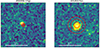 |
Fig. 1. 2″ × 2″ cutout images centred on the positions of the two SNe for which we detect a point source close to the SN position. ASASSN-17qp is displayed on the left and ATLAS17lsn on the right. In red the 1, 2 and 3σ uncertainties on the position of the SN are indicated. The centroid positions of the point sources that we considered to be potential SN detections are marked by white crosses. For ASSASN-17qp the white cross is just outside the 3σ uncertainty region, however, in Section 4.1 we discuss why we still consider this a possible detection of the SN. In both images north is up and east is left. |
For 36 SNe, no point source is detected within 3σ uncertainty of the SN position and for 13 SNe, we detected extended emission within (or close to) 3σ of the SN position; however, there is no detection of a point source on top of this extended emission. It is plausible that faint sources could be confused within the extended emission. However, our artificial star experiment accounts for this, and our limits for supernovae which lie on extended emission are correspondingly brighter. Table A.1 lists the full sample of SNe including upper limits for sources with non-detections and Figure B.111 shows a 1″ or 4″ cutout centred on the SN position with the 1, 2 and 3σ uncertainty region indicated in red circles.
The two SNe for which we may possibly still detect emission related to the SN are ASASSN-17qp/SN2017ivv and ATLAS17lsn/SN2017hcc. Both of these supernovae were previously identified as interacting events (Gutiérrez et al. 2020; Smith & Andrews 2020) and so, they are amongst the most likely systems for late-time UV detections. In Figure B.112, there is also a faint detection within the error region of SN2018ant. We looked at the individual _flc images to check if the source is an artefact from cosmic ray removal before combining the images. In the individual images, there is a cosmic ray at/near the position of the detection in two of the three images; in the third one, there is no source visible (see Figure C.113). We also use ASTRODRIZZLE to re-drizzle and combine the images, using driz_cr_grow = 3 for better cosmic ray removal. This produces an image without detection of a point source in the uncertainty region of the SN position. There has also been no mention of this SN as a long-term emitter in the literature. For SN2018ant we therefore assume this faint detection is not a real source.
Figure 2 shows the upper limits on the detection of a UV counterpart to the sample of SNe as a function of time since discovery. The light blue markers represent SNe where we detect no extended emission around or at the position of the SN, while the orange markers represent SNe where extended emission around the position of the SNe was detected in the HST images. While the events with extended diffuse emission typically yield brighter limiting magnitudes, the range of distances is such that this is not obvious in the absolute magnitude distribution. SNe for which a point source was detected inside the 3σ positional uncertainty region of the SN are marked by green squares with error bars. For comparison, the light curve of AT2018cow is also plotted in two filters close to the F275W filter used on this work.
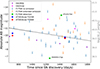 |
Fig. 2. Brightness of our sample of SNe versus time since discovery. The light curve of AT2018cow from Inkenhaag et al. (2023) at late times is plotted as well for comparison with circular markers in blue (F225W) and red (F336W). The black line represent the late time UV (UVW2-filter) brightness of the model with CSM interaction from Dessart et al. (2023), and the dashed line is the model extrapolated with the same decay rate for the duration of our observations. The light blue arrows represent upper limits to SNe emission determined close to/at the position of the SN, while orange arrows represent upper limits to SNe where there is extended emission close to/at the position of the SN. Light green squares indicate the magnitude of the detection of a point source in the UV at late times at a position consistent with that of the SN. They are labelled with the corresponding SN name and the error on the magnitude is smaller than the marker size. The magenta and purple stars are synthetic photometric measurements of SN2010jl and SN1993J, respectively, see the main text for details on how these were obtained. On the right axis, we have added the shock luminosity of the SN in erg s−1 corresponding to the absolute magnitude on the left axis for clarity. |
4. Discussion
We did not detect a point source within the 3σ uncertainty region for 49 of our 51 SNe, which corresponds to 96 percent of the cases. For 2 out of 51 (4 percent) we did find a point source that could be related to late-time emission from the CCSN.
For 13 of the 49 SNe for which we did not find a point source, there is evidence for the presence of extended emission close to the SN position. As expected, the artificial star experiment demonstrates that point sources need to be brighter to be recovered, leading to a less deep magnitude upper limit when extended emission is present. Additionally, for the two cases with a point source detected we do not find extended emission close to the SN position. At the distances of ASASSN-17qp and ATLAS17lsn the PSF size of 1.9 pixels in F275W corresponds to size of ∼9 and ∼29 parsec, respectively. Combined, this means that a SF region is only detected at, or at close projection of, the position of 25 percent of the SNe in our sample (assuming all UV emission is from SF regions). This assumption is reasonable because emission in the UV is dominated by young, massive stars which are born in SF regions. However, the luminosity function of SF regions is steep (α ≲ −1.73; e.g. Cook et al. 2016; Santoro et al. 2022) and therefore we cannot detect all the SF regions in the SN host galaxies due to the distance to the host galaxy. Hence, we can say our calculated 25 percent of CCSNe near a SF region is a lower limit to this number, and we refrain from making comparisons to other works investigating SN associations with SF regions which are typically made on much more local samples.
To get a better understanding of the progenitors of CCSNe and the nature of the peculiar transients recently discovered, one can also study their environments (e.g. Kuncarayakti et al. 2013a,b, 2018; Galbany et al. 2016b; Anderson et al. 2015; Lyman et al. 2020). Studying the environments in UV specifically, provides a window into star formation and massive star populations. As we do not detect a point source in most of our images on timescales between two and five years after the discovery of the SNe, we conclude that this is suitable timescale to consider if investigating the local environment is the goal.
4.1. Point source detections
The two SNe for which we detected a point source are ASASSN-17qp/SN2017ivv (Type II) and ATLAS17lsn/SN2017hcc (Type IIn). Both of these SNe are hydrogen-rich and likely had a massive progenitor that has shed part of its envelope through stellar winds, creating CSM with which the SN ejecta can interact. This interaction is primarily visible through (enhanced) UV emission (Dessart & Hillier 2022). We discuss both cases individually below.
4.1.1. SN2017hcc/ATLAS17lsn
From Figure 1, we can see that ATLAS17lsn is detected in the 1σ uncertainty region. The source has a chance of a false positive due to the SN position coinciding with pre-existing emission out to the offset of the SN of 1.5 × 10⁻³.
Moran et al. (2023) reported emission for this source from the optical through to the IR for more than 1700 days after its discovery. They argued this late time emission is due to interaction between massive, dense CSM and the SN ejecta, creating a slow rise to peak and a very slow, long decay of the light curve. This SN is known to most likely have had a massive progenitor that lost ∼10 M⊙ of mass before the explosion, creating shells of circumstellar material with which the supernova ejecta is interacting (Smith & Andrews 2020). Mauerhan et al. (2023) confirmed the presence of CSM through the high polarisation in the emission of ATLAS17lsn. Our late-time UV detection of this source adds to the evidence for a strong interaction between the CSM and SN ejecta in this source, which was also reported by Moran et al. (2023).
For this source, we were not able to obtain an early time image in which the SN and multiple other sources (also seen in the HST image) were detected. Therefore, we were unable to perform relative astrometry for this source.
To check if the observed source could be due to a young stellar cluster, we use the PARSEC stellar evolutionary tracks (v1.2S, Bressan et al. 2012; Chen et al. 2014, 2015; Tang et al. 2014) and COLIBRI evolutionary tracks (Marigo et al. 2013; Rosenfield et al. 2016; Pastorelli et al. 2019, 2020) through the CMD3.7 web interface14 to simulate populations of 104 and 105 M⊙ in mass of ages between 5 × 10⁵ and 20 × 106 years with steps of 5 × 10⁵ years for two metallicities, [M/H] = 0 (Z = 0.0147) and [M/H] = −0.5 (Z = 0.0048). The web interface has the option to output magnitudes in many filters from instruments on currently operating satellites and telescopes, including HST WFC3/F275W. We calculate the total absolute AB magnitude of all stars in a cluster of a certain age, mass and metallicity to obtain the cluster magnitude. For the absolute magnitude we measure for the detected point source (−12.9 mag), there is no cluster of 104 M⊙ that has an absolute magnitude brighter than the detected point source for either metallicities. For clusters with a mass of 105 M⊙, for [M/H] = 0, those with ages between 2 × 10⁵ and 5 × 10⁵ years do reach an absolute magnitude level of brightness that is higher than the detected point source. For [M/H] = −0.5, those with ages between 2.5 × 10⁵ and 5 × 10⁵ years also reach this level. This means there are clusters bright enough in the WFC3/F275W filter that would be detected at the distance of ATLAS17lsn. However, any underlying cluster would have to be young and unusually heavy to explain our detection. Given the previous identification of this SN as interacting, we feel that a SN is a better explanation for this detection.
4.1.2. SN2017ivv/ASASSN-17qp
ASASSN-17qp is known as a long-term emitter with different light curve slopes between 100–350 days and after 450 days (untill at least the end of the observations at ∼700 days; Gutiérrez et al. 2020), of which the former is steeper than expected from the decay of 56Co and the latter is slower than expected of a source powered by the decay of 56Co. This slower decay can be explained by the presence of an additional power source, such as interaction with the CSM (Gutiérrez et al. 2020), which would be consistent with our detection of this source in the UV.
In the left panel in Figure 1, we can see the 3σ uncertainty region of the position of ASASSN-17qp does not overlap with the centroid of the potential SN detection. As mentioned before, we do not include the centroiding error of the original SN detection in the calculation of the uncertainty on the SN position. Since the error on the position of this SN is 0.028″, which is one of the smallest in the sample, it is conceivable the centroiding error is not negligible for this source. For this SN, 3σ = 0.084″, while the distance between the reported SN position and the centroid position of the point source is ∼0.09″, which means there is only a 0.006″ difference. Assuming the FWHM ≈ 1″ during the discovery observation (or in the follow-up observations done for the ASAS-SN sources), σcentroid > 0.006″ if in the discovery image the detection S/N < 70. It is conceivable the S/N was lower than 70, meaning the centroiding error was non-negligible when calculating the uncertainty in the position of this particular SN. We therefore consider this point source to be associated with the SN.
We obtained an (acquisition) image from the ESO archive. This image was taken on 2018 March 25, 103 days after the discovery, with the EFOSC2 instrument on the NTT. The SN is still detected on this image. We use IRAF to perform relative astrometry between this image and our HST images using the GEOMAP and GEOXYTRAN tasks to map the SN position on the ground based image to that on the HST image. Figure 3 shows the HST image, centred on the position of ASASSN-17qp, with the position of the SN obtained from the ground indicated by a white circle. The size of the white circle represents the 3σ RMS uncertainty of the GEOMAP transformation between the ground based image and our HST images, which is 2.8 pixels (0.11 arcsecs). The red circles show the 1, 2 and 3σ uncertainty region of the reported SN position. From Figure 3 we can clearly see that our detected source lies within the 3σ uncertainty region of the SN position as determined from the ground based image. The uncertainty region also overlaps with the 3σ uncertainty region of the full SN position as reported in Table A.1. We therefore conclude our detection is indeed most likely still the SN. The chance of a false positive due to the SN position coinciding with pre-existing emission out to the offset of the SN is 3 × 10⁻⁴.
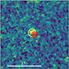 |
Fig. 3. Same as the left panel of Figure 1, except the white circle represents the projected position of a detection of ASASSN-17qp from a ground based image using relative astrometry. The size of the white circle is the 3σ uncertainty on the projected position, defined as the RMS of the solution of the mapping of the relative pixel positions of the stars in the ground based image to those of the HST image. North is up and east is left. |
For the simulated cluster absolute magnitudes as described above, all clusters in the age, mass and metallicity range reach an absolute magnitude brighter than the absolute magnitude of the detected point source (−6.7 mag). However, due to the proximity of ASASSN-17qp and its host galaxy, we would expect to see resolved clusters and not point sources. In this work we therefore assume this point source is associated with the SN.
4.2. Comparison to known interacting SNe
Our comparison of the detections of the interacting SNe in this work with those of well-known interacting SNe is hampered by the fact that the combination of late-time and UV imaging observations as presented here is unique. For example, SN2010jl has been observed for well over 1500 days, which is a similar timescale to our sample, but those observations were only done in optical filters. Fransson et al. (2014) report one measurement in the u′-band (their bluest band and close enough to the F275W filter to allow comparison) at 917 days of 19.16 ± 0.12 mag, which converts to an absolute magnitude of –14.28 ± 0.12 using the distance measure from Jencson et al. (2016). If we compare that to the upper limits plotted in Figure 2 we see that this particular SN would have been detected in all but one of the images, even on top of extended emission and even if the source would be slightly dimmer in the F275W filter. Another example, iPTF14hls, was monitored for more than 1200 days in optical by Sollerman et al. (2019), however, after ∼950 days there are no more observations in the bluest band in their data. SN2013L was also monitored up to 1500 days, but only in the ir-bands (Andrews et al. 2017).
There are, however, late-time UV spectroscopic measurements of SN2010jl, taken with the STIS instrument on board HST. The G230L(B) gratings cover the wavelength range of the WFC3/F275W filter used in this work. We obtain two spectra taken at 1224 and 1618 days and use the PYTHON package PYPHOT (v1.4.7; Fouesneau 2024) to perform synthetic photometry on these spectra. The obtained absolute magnitudes (corrected for Galactic extinction) are plotted in Figure 2, from which we can see that in the majority of images a SN similar to SN2010jl would have been detected. For another SN, SN1993J, there are late time UV-spectra obtained with the FOS instrument aboard HST (Fransson et al. 2005). We follow the same procedure to obtain synthetic photometric measurements in the WFC3/F275W filter from the spectra and added these measurements to Figure 2 as well. In the majority of the images, a SN similar to SN1993J would be below the detection limit and would therefore be undetected. SN1993J is less bright than SN2010jl and ATLAS17lsn at similar times, but brighter than ASASSN-17qp. This again supports the argument that there is a wide variety in the properties of interacting SNe and that more monitoring at late times is needed to fully understand the spectral and photometric characteristics of interacting SNe.
4.3. Comparison to interacting SN models
Comparing our work to models of CSM interacting SNe (from e.g. Dessart et al. 2023) is complicated without extensive modelling. However, we have over plotted the light curve from Dessart et al. (2023) in the UVW2-filter (which is similar to the F275W filter used in this work) presented in their Figure 3 in our light curve in Figure 2. The specific model that is discussed in detail in Dessart et al. (2023) is a 15.2 M⊙ star that evolves into a red super giant (RSG) and the resulting SN is injected with an extra power of 1040 erg s−1, corresponding with pre-SN wind of ∼10−6 M⊙ yr−1. For details on the other parameters such as mixing and the numerical setup, see Dessart et al. (2023) and references therein. Dessart et al. (2023) argue the amount of mass loss in this model is a typical value for a RSG and therefore the results are representative expectations for a standard Type II SN. Lower values of injected energy would imply a negligible impact of wind mass loss on the progenitor evolution. For different values of the injected power the effect on the brightness evolution is qualitatively similar. In respect to our work this means that more energy injection will mean a brighter UV source at later times, but is unclear from their work how much brighter, so we limit our self to comparing to their model discussed in detail. It does mean that the model we compare to can be considered a lower limit to the brightness for a star of this mass.
If we compare the model of Dessart et al. (2023) (represented by the black line until 1000 days and extrapolated with the same decay rate to later times in Figure 2) to the upper limits and detections we obtained, we can see that in roughly half of the images a SN as bright as this model would have been detected at late times. This means that for those images a non-detection does constrain the wind mass loss rate to being negligible, maybe even going as far as telling us that there was no CSM at the time of the SN. For the other upper limits a SN represented by this particular model would not have been detected as it is fainter than the upper limit of these images. We note that there are three images where this model would have been detected even on top of an extended emission region. SN2010jl is brighter than this model, but has a steeper decay rate between the two data points. SN1993C follows the same decay rate as the model, but is less bright. As we just argued that this particular model form Dessart et al. (2023) can be considered a lower limit on the luminosity, it is clear this model also does not represent SN2010jl in particular.
4.4. Implications for peculiar transient AT2018cow
Figure 2 allows us to compare the UV light curve of the CCSNe in our sample to the UV light curve of the peculiar transient AT2018cow and the interacting SN model from Dessart et al. (2023). Sun et al. (2022) were the first to report the presence of a UV bright source at the position of AT2018cow at late times (> 2 years), which they use to disfavour the origin of AT2018cow as a tidal disruption event (TDE). Comparing the magnitudes of the two possible SN detections in our sample to the light curve of AT2018cow, there is no evidence that the light curve of AT2018cow is atypical for interacting SNe. Comparing to the model from Dessart et al. (2023) mentioned before, we see that AT2018cow seems to decay slower than this model, but for the last epoch the magnitude is similar. However, there are many parameters in the models from Dessart et al. (2023) that can be changed (initial stellar mass, mixing parameters, shape of the CSM, etc.). Those parameters can influence the brightness and decay rate, so we cannot draw any firm conclusions from this comparison. 31 out of 49 of the SNe for which we do not detect a point source have a limiting magnitude brighter than AT2018cow, meaning a source as bright as AT2018cow can be present in these images without it being detected and the remaining 18 have a limiting magnitude fainter than AT2018cow at their respective observational epochs. Among the possible SN detections, one has a larger distance than AT2018cow (ATLAS17lsn), and one has a smaller distance (ASASSN-17qp). ATLAS17lsn has an absolute magnitude ∼3 magnitudes brighter than AT2018cow, while ASASSN-17qp has an absolute magnitude that is ∼3 magnitudes fainter than AT2018cow. Combined, this means the presence of late-time UV emission in AT2018cow is not an argument against a SN nature of this event. The difference in Δt (the time between discovery and the reported detection in this work) between the observations of AT2018cow and the detected SNe are not relevant for the conclusion, given the slow light curve evolution of AT2018cow.
If we limit the sample to SNe closer than AT2018cow, we can investigate if sources as bright as AT2018cow would have been detected if present or if emission as bright as AT2018cow would fall under the detection limit of the respective image. For emission as bright as AT2018cow at distances closer than AT2018cow, we would expect the emission to be brighter than the limiting magnitudes of the images under normal circumstances and so limiting to this distance range is a good probe of whether or not AT2018cow is unusually bright compared to the other CCSNe in this distance range. Only 5 out of 17 CCSNe have an absolute magnitude (limit) brighter than AT2018cow and the remaining 12 have a fainter limit (see Fig. D.1 in the supplementary material15). For this smaller sample it means that SNe as bright as AT2018cow would have been detected in 75 percent of the images. The model of Dessart et al. (2023) would also have been detected in 75 percent of the images, and as we do not detect a SN in this many images, we conclude AT2018cow is brighter than we would expect for CCSNe out to the distance of AT2018cow. This is an argument against a SN nature for AT2018cow.
AT2018cow is a black body (BB) with a very small radius (∼40 R⊙ at 713 and 1474 days; Inkenhaag et al. 2023). For any SN with CSM, if it is a BB at these epochs, then the photosphere is in the CSM, which means the radius will be bigger than 40 Rsun (e.g. Fassia et al. 2001; Smith et al. 2010; Kumar et al. 2019; Wang et al. 2023; Sfaradi et al. 2024). Therefore AT2018cow is unlikely to be a CCSN. This is in agreement with Liu et al. (2018), for instance.
5. Conclusions
Using our sample of 51 CCSNe observations, we found only two point source detections in HST data taken between two and five years after discovery. The absolute UV magnitude of the two detections compared to the late-time absolute UV magnitude of AT2018cow provides no evidence that the late-time UV detection of AT2018cow is an argument against it being a SN. However, AT2018cow is bright when compared to the subset of our CCSNe sample located at a distance closer than AT2018cow. Combined with the photospheric radius of AT2018cow’s emission being orders of magnitude smaller than that of CCSNe, we conclude that the late-time UV emission of AT2018cow is not likely to be driven by interaction. One explanation for its late-time UV emission is that we are viewing the inner region of the explosion, which could be a long-lived accretion disk. Such a scenario is expected in TDE models and it is less likely in SN scenarios.
These two detections represent some of the first UV detections of core collapse supernovae at late times after the explosion. Both SNe were also previously reported as interacting SNe, which means the late-time emission may be explained by continuing interaction between the SNe ejecta and the CSM that is expelled by the progenitor before the explosion (e.g. Dessart & Hillier 2022; Dessart et al. 2023). While we know the percentage of interacting SNe is ∼10 percent (e.g. Li et al. 2011; Smith et al. 2011), obtaining multiple epochs of UV imaging, in different bands, with contemporaneous spectra and detailed modelling will be necessary to fully understand these events (see Fransson et al. 2014 for a good example of what can be achieved). In most SNe, timescales of two to five years after explosion are therefore also suitable for investigating the SN environment. Furthermore, archival searches to look for detections of the progenitor star will give more direct information about the type of stars that can create these interacting SNe and offer information about the evolutionary stages in which CSM creation happens.
Data availability
Supplementary material is available at https://zenodo.org/records/14141215. All data used in this paper is publicly available from the HST data archive. Scripts and parameter files are available from the first author upon reasonable request.
See footnote 2.
See footnote 2.
The coordinates were obtained from the NED database: https://ned.ipac.caltech.edu/
Provided in the supplementary material available at https://zenodo.org/records/14141215
See footnote 11.
See footnote 11.
See footnote 11.
Acknowledgments
A.I. would like to thank Zheng Cao for helpful discussions about the sizes of the emission regions. The authors would like to thank the anonymous referee for the feedback provided, which has significantly improved the paper. This work is part of the research programme Athena with project number 184.034.002, which is financed by the Dutch Research Council (NWO). The scientific results reported on in this article are based on data obtained under HST Proposal 16287 with PI J.D. Lyman. P.G.J. has received funding from the European Research Council (ERC) under the European Union’s Horizon 2020 research and innovation programme (Grant agreement No. 101095973). M.F. is supported by a Royal Society - Science Foundation Ireland University Research Fellowship. J.D.L. acknowledges support from a UK Research and Innovation Future Leaders Fellowship (MR/T020784/1). L.G. acknowledges financial support from the Spanish Ministerio de Ciencia e Innovación (MCIN) and the Agencia Estatal de Investigación (AEI) 10.13039/501100011033 under the PID2020-115253GA-I00 HOSTFLOWS project, from Centro Superior de Investigaciones Científicas (CSIC) under the PIE project 20215AT016 and the program Unidad de Excelencia María de Maeztu CEX2020-001058-M, and from the Departament de Recerca i Universitats de la Generalitat de Catalunya through the 2021-SGR-01270 grant. H.K. was funded by the Research Council of Finland projects 324504, 328898, and 353019. This work makes use of Python packages NUMPY (Harris et al. 2020), SCIPY (Virtanen et al. 2020); MATPLOTLIB (Hunter 2007), EXTINCTION (Barbary 2016) and PANDAS (v1.3.5; McKinney 2010; the pandas development team 2014) This work made use of Astropy (http://www.astropy.org): a community-developed core Python package and an ecosystem of tools and resources for astronomy (Astropy Collaboration 2013, 2018, 2022).
References
- Anderson, J. P., González-Gaitán, S., Hamuy, M., et al. 2014, ApJ, 786, 67 [Google Scholar]
- Anderson, J. P., James, P. A., Habergham, S. M., Galbany, L., & Kuncarayakti, H. 2015, PASA, 32, e019 [NASA ADS] [CrossRef] [Google Scholar]
- Andrews, J. E., Smith, N., McCully, C., et al. 2017, MNRAS, 471, 4047 [Google Scholar]
- Arcavi, I., Hiramatsu, D., Jha, S. W., et al. 2018, ATel, 12135, 1 [NASA ADS] [Google Scholar]
- Astropy Collaboration (Robitaille, T. P., et al.) 2013, A&A, 558, A33 [NASA ADS] [CrossRef] [EDP Sciences] [Google Scholar]
- Astropy Collaboration (Price-Whelan, A. M., et al.) 2018, AJ, 156, 123 [Google Scholar]
- Astropy Collaboration (Price-Whelan, A. M., et al.) 2022, ApJ, 935, 167 [NASA ADS] [CrossRef] [Google Scholar]
- Barbary, K. 2016, https://doi.org/10.5281/zenodo.804967 [Google Scholar]
- Barbon, R., Ciatti, F., & Rosino, L. 1979, A&A, 72, 287 [Google Scholar]
- Bellm, E. C., Kulkarni, S. R., Graham, M. J., et al. 2019, PASP, 131, 018002 [Google Scholar]
- Benetti, S., Bufano, F., Vinko, J., et al. 2010, CBETs, 2536, 1 [NASA ADS] [Google Scholar]
- Bertin, E., & Arnouts, S. 1996, A&AS, 117, 393 [NASA ADS] [CrossRef] [EDP Sciences] [Google Scholar]
- Blagorodnova, N., Fremling, C., Neill, J. D., et al. 2018, ATel, 11493, 1 [NASA ADS] [Google Scholar]
- Blanchard, P., Nicholl, M., Berger, E., Fong, W., & Chornock, R. 2016, ATel, 8949, 1 [NASA ADS] [Google Scholar]
- Bloemen, S., Groot, P., Woudt, P., et al. 2016, in Ground-based and Airborne Telescopes VI, eds. H. J. Hall, R. Gilmozzi, & H. K. Marshall (International Society for Optics and Photonics (SPIE)), 9906, 990664 [NASA ADS] [CrossRef] [Google Scholar]
- Brennan, S. J., Elias-Rosa, N., Fraser, M., Van Dyk, S. D., & Lyman, J. D. 2022, A&A, 664, L18 [NASA ADS] [CrossRef] [EDP Sciences] [Google Scholar]
- Brennan, S. J., Schulze, S., Lunnan, R., et al. 2024, A&A, 690, A259 [NASA ADS] [CrossRef] [EDP Sciences] [Google Scholar]
- Bressan, A., Marigo, P., Girardi, L., et al. 2012, MNRAS, 427, 127 [NASA ADS] [CrossRef] [Google Scholar]
- Brown, J. S., & Foley, R. J. 2018, ATel, 12279, 1 [NASA ADS] [Google Scholar]
- Brown, P. J., Holland, S. T., Immler, S., et al. 2009, AJ, 137, 4517 [NASA ADS] [CrossRef] [Google Scholar]
- Castro-Segura, N., Pursiainen, M., Angus, C. R., et al. 2018, ATel, 12276, 1 [NASA ADS] [Google Scholar]
- Chen, Y., Girardi, L., Bressan, A., et al. 2014, MNRAS, 444, 2525 [Google Scholar]
- Chen, Y., Bressan, A., Girardi, L., et al. 2015, MNRAS, 452, 1068 [Google Scholar]
- Chevalier, R. A., & Fransson, C. 1994, ApJ, 420, 268 [NASA ADS] [CrossRef] [Google Scholar]
- Cook, D. O., Dale, D. A., Lee, J. C., et al. 2016, MNRAS, 462, 3766 [NASA ADS] [CrossRef] [Google Scholar]
- Coulter, D. A., Rojas-Bravo, C., Xhakaj, E., et al. 2017, ATel, 10593, 1 [NASA ADS] [Google Scholar]
- Crowther, P. A. 2007, ARA&A, 45, 177 [Google Scholar]
- Dessart, L. 2024, arXiv e-prints [arXiv:2405.04259] [Google Scholar]
- Dessart, L., & Hillier, D. J. 2022, A&A, 660, L9 [NASA ADS] [CrossRef] [EDP Sciences] [Google Scholar]
- Dessart, L., Audit, E., & Hillier, D. J. 2015, MNRAS, 449, 4304 [Google Scholar]
- Dessart, L., Gutiérrez, C. P., Kuncarayakti, H., Fox, O. D., & Filippenko, A. V. 2023, A&A, 675, A33 [NASA ADS] [CrossRef] [EDP Sciences] [Google Scholar]
- Dimitriadis, G., Pursiainen, M., Smith, M., et al. 2016, ATel, 9660, 1 [NASA ADS] [Google Scholar]
- Doggett, J. B., & Branch, D. 1985, AJ, 90, 2303 [Google Scholar]
- Dolphin, A. E. 2000, PASP, 112, 1383 [Google Scholar]
- Dong, S., Bersier, D., & Prieto, J. L. 2017, TNS Classif. Rep., 2017-1103, 1 [Google Scholar]
- Dong, Y., Valenti, S., Ashall, C., et al. 2024, ApJ, 974, 316 [NASA ADS] [CrossRef] [Google Scholar]
- Drake, A. J., Djorgovski, S. G., Mahabal, A., et al. 2009, ApJ, 696, 870 [Google Scholar]
- Draper, P. W., Gray, N., Berry, D. S., & Taylor, M. 2014, Astrophysics Source Code Library [record ascl:1403.024] [Google Scholar]
- Dugas, A., Fremling, C., Sharma, Y., et al. 2018, ATel, 12021, 1 [NASA ADS] [Google Scholar]
- Eappachen, D., Jonker, P. G., Fraser, M., et al. 2022, MNRAS, 514, 302 [NASA ADS] [CrossRef] [Google Scholar]
- Eldridge, J. J., Izzard, R. G., & Tout, C. A. 2008, MNRAS, 384, 1109 [Google Scholar]
- Elias, J. H., Matthews, K., Neugebauer, G., & Persson, S. E. 1985, ApJ, 296, 379 [NASA ADS] [CrossRef] [Google Scholar]
- Ercolino, A., Jin, H., Langer, N., & Dessart, L. 2024, A&A, 685, A58 [NASA ADS] [CrossRef] [EDP Sciences] [Google Scholar]
- Falco, E., Calkins, M., Challis, P., et al. 2016, ATel, 9237, 1 [NASA ADS] [Google Scholar]
- Fassia, A., Meikle, W. P. S., Chugai, N., et al. 2001, MNRAS, 325, 907 [NASA ADS] [CrossRef] [Google Scholar]
- Fouesneau, M. 2024, https://doi.org/10.5281/zenodo.7016774 [Google Scholar]
- Fox, O. D., & Smith, N. 2019, MNRAS, 488, 3772 [Google Scholar]
- Fransson, C. 1984, A&A, 133, 264 [NASA ADS] [Google Scholar]
- Fransson, C., Challis, P. M., Chevalier, R. A., et al. 2005, ApJ, 622, 991 [NASA ADS] [CrossRef] [Google Scholar]
- Fransson, C., Ergon, M., Challis, P. J., et al. 2014, ApJ, 797, 118 [Google Scholar]
- Fraser, M., Reynolds, T., Inserra, C., & Yaron, O. 2016, TNS Classif. Rep., 2016-490, 1 [Google Scholar]
- Fraser, M., Stritzinger, M. D., Brennan, S. J., et al. 2021, arXiv e-prints [arXiv:2108.07278] [Google Scholar]
- Frohmaier, C., Dimitriadis, G., Firth, R., et al. 2016, ATel, 8498, 1 [NASA ADS] [Google Scholar]
- Galbany, L., Hamuy, M., Phillips, M. M., et al. 2016a, AJ, 151, 33 [NASA ADS] [CrossRef] [Google Scholar]
- Galbany, L., Anderson, J. P., Rosales-Ortega, F. F., et al. 2016b, MNRAS, 455, 4087 [NASA ADS] [CrossRef] [Google Scholar]
- Gal-Yam, A. 2012, Science, 337, 927 [Google Scholar]
- Gal-Yam, A., Bruch, R., Schulze, S., et al. 2022, Nature, 601, 201 [NASA ADS] [CrossRef] [Google Scholar]
- Ginsburg, A., Sipőcz, B. M., Brasseur, C. E., et al. 2019, AJ, 157, 98 [Google Scholar]
- Gompertz, B. P., Cutter, R., Steeghs, D., et al. 2020, MNRAS, 497, 726 [NASA ADS] [CrossRef] [Google Scholar]
- Gutierrez, C. P., Cartier, R., Smith, M., et al. 2017a, ATel, 10338, 1 [NASA ADS] [Google Scholar]
- Gutierrez, C. P., Cartier, R., Smith, M., et al. 2017b, ATel, 10318, 1 [NASA ADS] [Google Scholar]
- Gutierrez, C. P., Cartier, R., Smith, M., et al. 2017c, ATel, 10331, 1 [NASA ADS] [Google Scholar]
- Gutiérrez, C. P., Pastorello, A., Jerkstrand, A., et al. 2020, MNRAS, 499, 974 [CrossRef] [Google Scholar]
- Harris, C. R., Millman, K. J., van der Walt, S. J., et al. 2020, Nature, 585, 357 [NASA ADS] [CrossRef] [Google Scholar]
- Hiramatsu, D., Howell, D. A., Moriya, T. J., et al. 2021, ApJ, 913, 55 [CrossRef] [Google Scholar]
- Holoien, T. W. S., Brown, J. S., Stanek, K. Z., et al. 2017a, MNRAS, 471, 4966 [NASA ADS] [CrossRef] [Google Scholar]
- Holoien, T. W. S., Stanek, K. Z., Kochanek, C. S., et al. 2017b, MNRAS, 464, 2672 [NASA ADS] [CrossRef] [Google Scholar]
- Holoien, T. W. S., Brown, J. S., Stanek, K. Z., et al. 2017c, MNRAS, 467, 1098 [NASA ADS] [Google Scholar]
- Holoien, T. W. S., Brown, J. S., Vallely, P. J., et al. 2019, MNRAS, 484, 1899 [NASA ADS] [CrossRef] [Google Scholar]
- Homan, D., Lyman, J., Galbany, L., et al. 2017, ATel, 10676, 1 [NASA ADS] [Google Scholar]
- Hosseinzadeh, G., Howell, D. A., Arcavi, I., Mccully, C., & Valenti, S. 2016, TNS Classif. Rep., 2016-785, 1 [Google Scholar]
- Hunter, J. D. 2007, Comput. Sci. Eng., 9, 90 [NASA ADS] [CrossRef] [Google Scholar]
- Inkenhaag, A., Jonker, P. G., Levan, A. J., et al. 2023, MNRAS, 525, 4042 [NASA ADS] [CrossRef] [Google Scholar]
- Inserra, C. 2019, Nat. Astron., 3, 697 [NASA ADS] [CrossRef] [Google Scholar]
- Ivezić, Ž., Kahn, S. M., Tyson, J. A., et al. 2019, ApJ, 873, 111 [Google Scholar]
- Jencson, J. E., Prieto, J. L., Kochanek, C. S., et al. 2016, MNRAS, 456, 2622 [NASA ADS] [CrossRef] [Google Scholar]
- Kasliwal, M. M., Kulkarni, S. R., Gal-Yam, A., et al. 2012, ApJ, 755, 161 [NASA ADS] [CrossRef] [Google Scholar]
- Kawabata, M. 2017, TNS Classif. Rep., 2017-1458, 1 [Google Scholar]
- Kostrzewa-Rutkowska, Z., Lopez, K. M., Cannizzaro, G., et al. 2017, ATel, 11024, 1 [NASA ADS] [Google Scholar]
- Kostrzewa-Rutkowska, Z., Jonker, P. G., Hodgkin, S. T., et al. 2018, MNRAS, 481, 307 [CrossRef] [Google Scholar]
- Kuin, N. P. M., Wu, K., Oates, S., et al. 2019, MNRAS, 487, 2505 [NASA ADS] [CrossRef] [Google Scholar]
- Kumar, B., Eswaraiah, C., Singh, A., et al. 2019, MNRAS, 488, 3089 [NASA ADS] [CrossRef] [Google Scholar]
- Kuncarayakti, H., Doi, M., Aldering, G., et al. 2013a, AJ, 146, 30 [NASA ADS] [CrossRef] [Google Scholar]
- Kuncarayakti, H., Doi, M., Aldering, G., et al. 2013b, AJ, 146, 31 [NASA ADS] [CrossRef] [Google Scholar]
- Kuncarayakti, H., Anderson, J. P., Galbany, L., et al. 2018, A&A, 613, A35 [NASA ADS] [CrossRef] [EDP Sciences] [Google Scholar]
- Leung, S.-C., Blinnikov, S., Nomoto, K., et al. 2020, ApJ, 903, 66 [NASA ADS] [CrossRef] [Google Scholar]
- Li, W., Leaman, J., Chornock, R., et al. 2011, MNRAS, 412, 1441 [NASA ADS] [CrossRef] [Google Scholar]
- Liu, L.-D., Zhang, B., Wang, L.-J., & Dai, Z.-G. 2018, ApJ, 868, L24 [NASA ADS] [CrossRef] [Google Scholar]
- Lyman, J., Homan, D., Magee, M., et al. 2017a, ATel, 10650, 1 [NASA ADS] [Google Scholar]
- Lyman, J., Homan, D., Galbany, L., et al. 2017b, ATel, 10674, 1 [NASA ADS] [Google Scholar]
- Lyman, J. D., Galbany, L., Sánchez, S. F., et al. 2020, MNRAS, 495, 992 [NASA ADS] [CrossRef] [Google Scholar]
- Magee, M., Bar, I., Leloudas, G., et al. 2016, ATel, 8963, 1 [NASA ADS] [Google Scholar]
- Magnier, E. A., Schlafly, E. F., Finkbeiner, D. P., et al. 2020, ApJS, 251, 6 [NASA ADS] [CrossRef] [Google Scholar]
- Maguire, K. 2017, in Handbook of Supernovae, eds. A. W. Alsabti, & P. Murdin, 293 [CrossRef] [Google Scholar]
- Margutti, R., Metzger, B. D., Chornock, R., et al. 2019, ApJ, 872, 18 [Google Scholar]
- Marigo, P., Bressan, A., Nanni, A., Girardi, L., & Pumo, M. L. 2013, MNRAS, 434, 488 [Google Scholar]
- Mauerhan, J. C., Smith, N., Williams, G. G., et al. 2023, MNRAS, submitted [arXiv:2304.12368] [Google Scholar]
- McKinney, W. 2010, in Proceedings of the 9th Python in Science Conference (Austin, TX), 445, 51 [Google Scholar]
- Metzger, B. D. 2022, ApJ, 932, 84 [NASA ADS] [CrossRef] [Google Scholar]
- Minkowski, R. 1941, PASP, 53, 224 [NASA ADS] [CrossRef] [Google Scholar]
- Modjaz, M., Liu, Y. Q., Bianco, F. B., & Graur, O. 2016, ApJ, 832, 108 [NASA ADS] [CrossRef] [Google Scholar]
- Mohan, P., An, T., & Yang, J. 2020, ApJ, 888, L24 [NASA ADS] [CrossRef] [Google Scholar]
- Monard, L. A. G., Morales Garoffolo, A., Elias-Rosa, N., et al. 2013, CBETs, 3392, 1 [NASA ADS] [Google Scholar]
- Moran, S., Fraser, M., Kotak, R., et al. 2023, A&A, 669, A51 [NASA ADS] [CrossRef] [EDP Sciences] [Google Scholar]
- Morrell, N., Shappee, B., Drout, M., & Dong, S. 2017, ATel, 10240, 1 [NASA ADS] [Google Scholar]
- Neumann, K. D., Holoien, T. W. S., Kochanek, C. S., et al. 2023, MNRAS, 520, 4356 [NASA ADS] [CrossRef] [Google Scholar]
- Newton, J., & Puckett, T. 2010, CBETs, 2532, 1 [NASA ADS] [Google Scholar]
- Nomoto, K., Thielemann, F. K., & Yokoi, K. 1984, ApJ, 286, 644 [Google Scholar]
- Ochner, P., Benetti, S., Cappellaro, E., Tomasella, L., & Turatto, M. 2017, ATel, 11063, 1 [NASA ADS] [Google Scholar]
- Ofek, E. O., Cameron, P. B., Kasliwal, M. M., et al. 2007, ApJ, 659, L13 [CrossRef] [Google Scholar]
- Onori, F., Cannizzaro, G., Kostrzewa-Rutkowska, Z., et al. 2017, ATel, 10964, 1 [NASA ADS] [Google Scholar]
- Onori, F., Stein, R., Cannizzaro, G., et al. 2018, ATel, 11916, 1 [NASA ADS] [Google Scholar]
- Pastorelli, G., Marigo, P., Girardi, L., et al. 2019, MNRAS, 485, 5666 [Google Scholar]
- Pastorelli, G., Marigo, P., Girardi, L., et al. 2020, MNRAS, 498, 3283 [Google Scholar]
- Pastorello, A., Smartt, S. J., Mattila, S., et al. 2007, Nature, 447, 829 [NASA ADS] [CrossRef] [Google Scholar]
- Pellegrino, C., Howell, D. A., Vinkó, J., et al. 2022, ApJ, 926, 125 [NASA ADS] [CrossRef] [Google Scholar]
- Perley, D. A., Mazzali, P. A., Yan, L., et al. 2019, MNRAS, 484, 1031 [Google Scholar]
- Perley, D. A., Sollerman, J., Schulze, S., et al. 2022, ApJ, 927, 180 [NASA ADS] [CrossRef] [Google Scholar]
- Pignata, G., Wang, L., Galbany, L., et al. 2017, ATel, 10454, 1 [NASA ADS] [Google Scholar]
- Planck Collaboration XIII. 2016, A&A, 594, A13 [NASA ADS] [CrossRef] [EDP Sciences] [Google Scholar]
- Podsiadlowski, P., Joss, P. C., & Hsu, J. J. L. 1992, ApJ, 391, 246 [Google Scholar]
- Prentice, S. J., Maguire, K., Smartt, S. J., et al. 2018a, ApJ, 865, L3 [NASA ADS] [CrossRef] [Google Scholar]
- Prentice, S. J., Maguire, K., Smartt, S. J., et al. 2018b, ATel, 12014, 1 [NASA ADS] [Google Scholar]
- Prieto, J. L., & Shappee, B. J. 2017, TNS Classif. Rep., 2017-259, 1 [Google Scholar]
- Pritchard, T. A., Roming, P. W. A., Brown, P. J., Bayless, A. J., & Frey, L. H. 2014, ApJ, 787, 157 [NASA ADS] [CrossRef] [Google Scholar]
- Quimby, R. 2006, CBETs, 644, 1 [NASA ADS] [Google Scholar]
- Quimby, R. M., Kulkarni, S. R., Kasliwal, M. M., et al. 2011, Nature, 474, 487 [NASA ADS] [CrossRef] [Google Scholar]
- Rodriguez, O., & Prieto, J. L. 2017a, ATel, 10580, 1 [NASA ADS] [Google Scholar]
- Rodriguez, O., & Prieto, J. L. 2017b, ATel, 10586, 1 [NASA ADS] [Google Scholar]
- Rojas-Bravo, C., Coulter, D. A., Siebert, M. R., & Foley, J. 2018, ATel, 11914, 1 [NASA ADS] [Google Scholar]
- Rosenfield, P., Marigo, P., Girardi, L., et al. 2016, ApJ, 822, 73 [NASA ADS] [CrossRef] [Google Scholar]
- Sahu, D. K., Anupama, G. C., Chakradhari, N. K., et al. 2018, MNRAS, 475, 2591 [NASA ADS] [CrossRef] [Google Scholar]
- Sanders, N. E., Soderberg, A. M., Gezari, S., et al. 2015, ApJ, 799, 208 [NASA ADS] [CrossRef] [Google Scholar]
- Santoro, F., Kreckel, K., Belfiore, F., et al. 2022, A&A, 658, A188 [NASA ADS] [CrossRef] [EDP Sciences] [Google Scholar]
- Schlafly, E. F., & Finkbeiner, D. P. 2011, ApJ, 737, 103 [Google Scholar]
- Schlegel, E. M. 1990, MNRAS, 244, 269 [NASA ADS] [Google Scholar]
- Schlegel, D. J., Finkbeiner, D. P., & Davis, M. 1998, ApJ, 500, 525 [Google Scholar]
- Sfaradi, I., Horesh, A., Sollerman, J., et al. 2024, A&A, 686, A129 [NASA ADS] [CrossRef] [EDP Sciences] [Google Scholar]
- Shappee, B. J., Prieto, J. L., Grupe, D., et al. 2014, ApJ, 788, 48 [Google Scholar]
- Siebert, M. R., Coulter, D. A., Kilpatrick, C. D., et al. 2017, ATel, 10582, 1 [NASA ADS] [Google Scholar]
- Smartt, S. J. 2009, ARA&A, 47, 63 [NASA ADS] [CrossRef] [Google Scholar]
- Smith, N., & Andrews, J. E. 2020, MNRAS, 499, 3544 [NASA ADS] [CrossRef] [Google Scholar]
- Smith, N., & Arnett, W. D. 2014, ApJ, 785, 82 [NASA ADS] [CrossRef] [Google Scholar]
- Smith, N., Li, W., Foley, R. J., et al. 2007, ApJ, 666, 1116 [NASA ADS] [CrossRef] [Google Scholar]
- Smith, N., Chornock, R., Silverman, J. M., Filippenko, A. V., & Foley, R. J. 2010, ApJ, 709, 856 [NASA ADS] [CrossRef] [Google Scholar]
- Smith, N., Li, W., Filippenko, A. V., & Chornock, R. 2011, MNRAS, 412, 1522 [NASA ADS] [CrossRef] [Google Scholar]
- Smith, K., Cikota, A., Magee, M., Inserra, C., & Yaron, O. 2017, TNS Classif. Rep., 2017-27, 1 [Google Scholar]
- Smith, K., Palmerio, J., O’Neill, D., et al. 2018, ATel, 11294, 1 [NASA ADS] [Google Scholar]
- Sollerman, J., Taddia, F., Arcavi, I., et al. 2019, A&A, 621, A30 [NASA ADS] [CrossRef] [EDP Sciences] [Google Scholar]
- Somero, A., Kuncarayakti, H., Mattila, S., et al. 2017, ATel, 10594, 1 [NASA ADS] [Google Scholar]
- Steeghs, D., Galloway, D. K., Ackley, K., et al. 2022, MNRAS, 511, 2405 [NASA ADS] [CrossRef] [Google Scholar]
- Stoll, R., Prieto, J. L., Stanek, K. Z., et al. 2011, ApJ, 730, 34 [NASA ADS] [CrossRef] [Google Scholar]
- Stritzinger, M. D., Fraser, M., Hummelmose, N. N., et al. 2017, ATel, 10672, 1 [NASA ADS] [Google Scholar]
- Sun, N.-C., Maund, J. R., Crowther, P. A., & Liu, L.-D. 2022, MNRAS, 512, L66 [NASA ADS] [CrossRef] [Google Scholar]
- Taddia, F., Sollerman, J., Barbarino, C., et al. 2017, ATel, 10012, 1 [NASA ADS] [Google Scholar]
- Tang, J., Bressan, A., Rosenfield, P., et al. 2014, MNRAS, 445, 4287 [NASA ADS] [CrossRef] [Google Scholar]
- Tartaglia, L., Valenti, S., Bostroem, K. A., Yang, S., & Hosseinzadeh, G. 2017, ATel, 10603, 1 [NASA ADS] [Google Scholar]
- the pandas development team 2014, https://doi.org/10.5281/zenodo.5774815 [Google Scholar]
- Tody, D. 1986, SPIE Conf. Ser., 627, 733 [Google Scholar]
- Tody, D. 1993, ASP Conf. Ser., 52, 173 [NASA ADS] [Google Scholar]
- Tomasella, L. 2018, TNS Classif. Rep., 2018-2072, 1 [Google Scholar]
- Tomasella, L., Benetti, S., & Cappellaro, E. 2017, ATel, 10680, 1 [NASA ADS] [Google Scholar]
- Tonry, J. L. 2011, PASP, 123, 58 [NASA ADS] [CrossRef] [Google Scholar]
- Tonry, J. L., Denneau, L., Heinze, A. N., et al. 2018, PASP, 130, 064505 [Google Scholar]
- Uddin, S., Mould, J., Zhang, J.-J., Wang, L., & Wang, X. 2017, ATel, 10769, 1 [NASA ADS] [Google Scholar]
- Van Dyk, S. D., Zheng, W., Shivvers, I., et al. 2016, ATel, 9573, 1 [NASA ADS] [Google Scholar]
- Vink, J. S., de Koter, A., & Lamers, H. J. G. L. M. 2001, A&A, 369, 574 [NASA ADS] [CrossRef] [EDP Sciences] [Google Scholar]
- Virtanen, P., Gommers, R., Oliphant, T. E., et al. 2020, Nat. Methods, 17, 261 [Google Scholar]
- Wang, T., Wang, S.-Q., Gan, W.-P., & Li, L. 2023, ApJ, 948, 138 [NASA ADS] [CrossRef] [Google Scholar]
- Wheeler, J. C., & Harkness, R. P. 1986, in NATO Advanced Study Institute (ASI) Series C, eds. B. F. Madore, & R. B. Tully, Galaxy Distances and Deviations from Universal Expansion, 180, 45 [NASA ADS] [Google Scholar]
- Woosley, S. E., & Weaver, T. A. 1986, ARA&A, 24, 205 [NASA ADS] [CrossRef] [Google Scholar]
- Woosley, S. E., Pinto, P. A., Martin, P. G., & Weaver, T. A. 1987, ApJ, 318, 664 [NASA ADS] [CrossRef] [Google Scholar]
- Xhakaj, E., Rojas-Bravo, C., Foley, M. M., et al. 2017, ATel, 10620, 1 [NASA ADS] [Google Scholar]
- Xiang, D., Wang, X., Lin, W., et al. 2021, ApJ, 910, 42 [NASA ADS] [CrossRef] [Google Scholar]
- Xin, Y.-X., & Zhang, J.-J. 2016, ATel, 8540, 1 [NASA ADS] [Google Scholar]
- Yoshida, T., Takiwaki, T., Kotake, K., et al. 2021, ApJ, 908, 44 [NASA ADS] [CrossRef] [Google Scholar]
- Zhang, J., Xin, Y., Xiang, D., et al. 2016, ATel, 9746, 1 [NASA ADS] [Google Scholar]
- Zhang, J., Huang, F., & Wang, X. 2017a, TNS Classif. Rep., 2017-515, 1 [Google Scholar]
- Zhang, J., Yu, X., Li, W., et al. 2017b, ATel, 10336, 1 [NASA ADS] [Google Scholar]
Appendix A: Sample of supernovae
Full sample of SNe including relevant information used in this work.
All Tables
Errors on the reported positions of supernovae for various surveys and telescopes that have reported SNe used in this paper.
All Figures
|
Fig. 1. 2″ × 2″ cutout images centred on the positions of the two SNe for which we detect a point source close to the SN position. ASASSN-17qp is displayed on the left and ATLAS17lsn on the right. In red the 1, 2 and 3σ uncertainties on the position of the SN are indicated. The centroid positions of the point sources that we considered to be potential SN detections are marked by white crosses. For ASSASN-17qp the white cross is just outside the 3σ uncertainty region, however, in Section 4.1 we discuss why we still consider this a possible detection of the SN. In both images north is up and east is left. |
| In the text | |
|
Fig. 2. Brightness of our sample of SNe versus time since discovery. The light curve of AT2018cow from Inkenhaag et al. (2023) at late times is plotted as well for comparison with circular markers in blue (F225W) and red (F336W). The black line represent the late time UV (UVW2-filter) brightness of the model with CSM interaction from Dessart et al. (2023), and the dashed line is the model extrapolated with the same decay rate for the duration of our observations. The light blue arrows represent upper limits to SNe emission determined close to/at the position of the SN, while orange arrows represent upper limits to SNe where there is extended emission close to/at the position of the SN. Light green squares indicate the magnitude of the detection of a point source in the UV at late times at a position consistent with that of the SN. They are labelled with the corresponding SN name and the error on the magnitude is smaller than the marker size. The magenta and purple stars are synthetic photometric measurements of SN2010jl and SN1993J, respectively, see the main text for details on how these were obtained. On the right axis, we have added the shock luminosity of the SN in erg s−1 corresponding to the absolute magnitude on the left axis for clarity. |
| In the text | |
|
Fig. 3. Same as the left panel of Figure 1, except the white circle represents the projected position of a detection of ASASSN-17qp from a ground based image using relative astrometry. The size of the white circle is the 3σ uncertainty on the projected position, defined as the RMS of the solution of the mapping of the relative pixel positions of the stars in the ground based image to those of the HST image. North is up and east is left. |
| In the text | |
Current usage metrics show cumulative count of Article Views (full-text article views including HTML views, PDF and ePub downloads, according to the available data) and Abstracts Views on Vision4Press platform.
Data correspond to usage on the plateform after 2015. The current usage metrics is available 48-96 hours after online publication and is updated daily on week days.
Initial download of the metrics may take a while.