| Issue |
A&A
Volume 693, January 2025
|
|
|---|---|---|
| Article Number | A310 | |
| Number of page(s) | 18 | |
| Section | Planets, planetary systems, and small bodies | |
| DOI | https://doi.org/10.1051/0004-6361/202347194 | |
| Published online | 29 January 2025 | |
A general polarimetric model for transiting and nontransiting ringed exoplanets
1
Faculty of Aerospace Engineering, Technical University Delft,
Kluyverweg 1,
2629 HS
Delft,
The Netherlands
2
SEAP/FACom, Instituto de Física – FCEN, Universidad de Antioquia,
Calle 70 No. 52-21,
Medellín,
Colombia
3
School of Mathematical and Physical Sciences, Macquarie University,
Balaclava Road,
North Ryde,
NSW
2109,
Australia
4
The Macquarie University Astrophysics and Space Technologies Research Centre, Macquarie University,
Balaclava Road,
North Ryde,
NSW
2109,
Australia
5
Departamento de Ciencias, Facultad de Artes Liberales, Universidad Adolfo Ibáñez,
Av. Padre Hurtado 750,
Viña del Mar,
Chile
6
Univ. Grenoble Alpes, CNRS, IPAG,
38000
Grenoble,
France
7
Leiden Observatory, University of Leiden,
PO Box 9513,
2300 RA
Leiden,
The Netherlands
★ Corresponding authors; This email address is being protected from spambots. You need JavaScript enabled to view it.
; This email address is being protected from spambots. You need JavaScript enabled to view it.
; This email address is being protected from spambots. You need JavaScript enabled to view it.
Received:
15
June
2023
Accepted:
3
December
2024
Abstract
Context. The detection and characterization of exorings (rings around exoplanets) will help us to better understand the origin and evolution of planetary rings in the Solar System and beyond. However, exorings are still elusive, and new and clever methods for identifying them need to be developed and tested.
Aims. We explore the potential of polarimetry as a tool for discovering and characterizing exorings.
Methods. For this purpose, we improved the general publicly available photometric code Pryngles by adding the results of radiative transfer calculations with an adding-doubling algorithm that fully includes polarization. With this improved code, we computed the total and polarized fluxes and the degree of polarization of model gas giant planets with or without rings. Additionally, we demonstrate the versatility of our code by predicting the polarimetric signal of the puffed-up planet HIP 41378 f as if it had an exoring.
Results. Spatially unresolved dusty rings can significantly modify the flux and polarization signals of the light that is reflected by a gas giant exoplanet along its orbit. Rings are expected to have a low polarization signal, but they will decrease the degree of polarization of reflected light when they cast a shadow on the planet and/or block part of the planet. The most diagnostic feature of a ring occurs around the ring-plane crossings when sharp changes in the flux and degree of polarization curves are predicted by our model. When we applied our methods to HIP 41378 f, we found that if it is surrounded by a ring, noticeable changes in the degree of polarization of reflected light will arise. Although the reflected light on the planet cannot yet be directly imaged, the addition of polarimetry to future observations would aid in the characterization of the system.
Key words: polarization / methods: numerical / planets and satellites: rings
© The Authors 2025
 Open Access article, published by EDP Sciences, under the terms of the Creative Commons Attribution License (https://creativecommons.org/licenses/by/4.0), which permits unrestricted use, distribution, and reproduction in any medium, provided the original work is properly cited.
This article is published in open access under the Subscribe to Open model. This email address is being protected from spambots. You need JavaScript enabled to view it. to support open access publication.
1 Introduction
The discovery of planetary rings, hereafter exorings, remains elusive (see e.g. Piro & Vissapragada 2020 and references therein) for all exoplanets that were discovered so far, even though most of these planets are gas giants. Although the absence of exorings might seem like an unsolved mystery, it might be due to the limitations of the methods and techniques we use to detect them. The fainter rings around the giant planets in the Solar System, especially those of Jupiter, Uranus, and Neptune, were discovered through in situ observations by spacecraft, or through the detection of anomalies in the light curve of stellar occultations (Charnoz et al. 2018).
Current efforts to detect exorings using planetary transits have been unsuccessful thus far. One interesting explanation for this fact might be that the signal of many exorings is hidden among the trove of available photometric data, but is misinterpreted as large puffed-up planets (Zuluaga et al. 2015, 2022; Ohno & Fortney 2022). Ringed exoplanets would project a larger area on the stellar disk than an exoplanet without rings, and this type of exoplanet also has a larger apparent size when observed indirectly through planetary transits. To circumvent this problem, it has been suggested that rings might be detected in reflected light rather than during a transit (Arnold & Schneider 2004; Dyudina et al. 2005; Sucerquia et al. 2020). Planetary rings can contribute to a noticeable increase in stellar flux during most of their orbit and depending on the geometry of the system (Sucerquia et al. 2020; Lietzow & Wolf 2023). The detection of these photometric anomalies could reveal the presence of a ring and help us to characterize it.
Moreover, scattered light and polarization measurements have recently emerged as a crucial tool in the study of exoplanets. These measurements reveal valuable information about the properties of the exoplanet that cannot be obtained using traditional techniques. For instance, instruments such as the Spectro-Polarimetric High-contrast Exoplanet REsearch/Zurich IMaging POLarimeter (SPHERE/ZIMPOL) intend to use light that is polarized from planetary surfaces to characterize cold planets (Knutson et al. 2007; Schmid et al. 2018). Other studies have proposed similar methods for the detection and characterization of directly imaged exoplanets (see, e.g. Stam et al. 2004; Karalidi et al. 2012, 2013; Stolker et al. 2017). All of these techniques, along with the appropriate instruments, might help us understand the nature of many extrasolar systems whose behaviors are still awaiting an explanation. This is the case, for instance, of the phase curve of 55 Cancri, whose time-varying occultation depth (Tamburo et al. 2018; Morris et al. 2021; Meier Valdés et al. 2022) defies current models of light reflection and emission (Demory et al. 2023), or of the discovery of hot so-called puffed-up planets that appear to have extraordinarily low densities (Piro & Vissapragada 2020), such as HIP 41378 f (Akinsanmi et al. 2020; Alam et al. 2022).
In anticipation of these new instruments and measurement techniques, we continue our work on a numerical model, called Pryngles, that can model both the reflected light curve and the transit. In Zuluaga et al. (2022) we introduced Pryngles1, a novel Python package, and we fully implemented and tested the novel geometrical model that characterizes our approach, namely, a decomposition of the bodies into so-called spangles. The code uses a planetocentric description of the relative position of the star, planet, and ring. The original version used a simplified treatment of reflection and scattering and did not include polarization.
In this paper, we present, test, and apply an updated version of Pryngles that enables the computation of total and polarized fluxes and the degree and direction of polarization for ringed exoplanets. To accomplish this, we used realistic phase curves calculated by an adding-doubling radiative transfer algorithm (for the planetary atmospheres) and experimental data (for ring particles), which includes polarization at all orders of light scattering.
We used this updated model to investigate the effect of a ring on the reflected light and polarization curves. Recently, Lietzow & Wolf (2023) also modeled the total flux and polarization of light scattered by exoplanetary rings with a Monte Carlo algorithm. To distinguish our method from their method and results, we focused especially on the signal of a ringed planet that is not seen edge-on. This focus is not unfounded given the recent interest in better direct observations of planets (e.g. National Academies of Sciences, Engineering, and Medicine 2021). Another distinction and improvement is our use of nonspherical ring particles. Although the model by Lietzow & Wolf uses ring particles of different sizes and compositions, the authors assumed that all particles were homogeneous spherical particles, which generally show much stronger angular features in their single-scattering phase curves than more realistic irregularly shaped particles (see, e.g., Muñoz et al. 2000). In contrast, our single-scattering phase curves of the ring particles are based on laboratory measurements of light scattering by irregularly shaped particles (for a description of the experimental set-up, see Muñoz et al. 2012). This ensures a more accurate calculation of the reflected or transmitted light by the rings, although at the price of lacking the flexibility to change the composition and size of the ring particles.
This paper is organized as follows. In Section 2, we give a brief overview of the Pryngles package and describe the improvements implemented for this paper, and the physics behind them. We describe the physical properties of a set of model planets and their corresponding rings, which we use to test and demonstrate the capabilities of our model in Section 3. Section 4 presents the results of computing the fluxes and polarization curves for our model planets. Finally, we apply our model and tools to study the case of the possibly puffed-up planet HIP 41378 f. The results are summarized in Section 5. The limitations and prospects of this work are presented in Section 6, and in Section 7 we summarize and draw the main conclusions of our work.
2 Pryngles: Planets in spangles
In Figure 1, we illustrate the appearance of a ringed planet as represented in Pryngles and the corresponding geometrical configuration of a typical simulation. Although the representation in Figure 1 is centered on the star (filled white circle in the center), the model is initially planetocentric, which considerably simplifies the computation of the viewing and illumination conditions (see Zuluaga et al. 2022 and Appendix B for additional details).
2.1 Geometrical description of the system
The illumination and viewing geometries of the planetary and ring spangles vary with the location of the planet along its orbit, as measured by the true anomaly ν. For simplicity, we assume hereafter that the orbit of the planet is circular. As a result, true anomaly is arbitrarily defined with respect to the point in the planet orbit that is closest to the subobserver location. In all our simulations, at ν = 0° the planet therefore is between the observer and the star. In this specific configuration, we mostly observe the nightside of the planet.
The ring and orbital orientation are defined by the three angles that are schematically represented in Figure 2. They are the orbital inclination angle i (i = 90° corresponds to an edge-on orbit), the ring inclination angle γ with respect to the direction of the observer (γ = 90° corresponds to an edge-on ring), and the azimuthal rotation angle or roll angle λr .
A complimentary angle that is frequently mentioned when we describe our results, is the planetary phase angle α, which is defined as the angle between the direction toward the observer and the line joining the centers of the star and the planet (see Figure 2). If α = 0°, the planet is fully illuminated by the star (ignoring the possible influence of a ring and the fact that the planet would be precisely behind its star as seen by the observer). On the other hand, when α = 180°, the full nightside of the planet is in view, and in rigor, the planet would be transiting the stellar disk. The range of values that the phase angle can attain along the planet depends on the inclination angle i. Figure 2 cleary shows that 90° − i ≤ α ≤ 90° + i. With the exception of the case when i = 0° (a face-on orbit for which always α = 90°), the planetary phase angle α changes with the true anomaly ν.
2.2 Illumination and viewing conditions
Describing the color conventions we use in Pryngles graphical outputs, as illustrated in Figure 1, is key to understanding the different conditions of illumination and viewing of the spangles that determine the flux and polarization of light reflected by the planet and ring. For the system represented in Figure 1, the so-called ring-plane crossings, that is, the configuration when an infinitely thin ring neither reflects nor transmits stellar light, occur at ν = 90° and 270°. Ring spangles under this condition are represented in gray.
Along part of the orbit in the upper half of the figure (90° ≤ ν ≤ 270°), the shadow of the ring on the planet reveals that the ring is seen in diffusely transmitted starlight (the star illuminates the bottom of the ring as seen from the observer). In Pryngles we show the spangles under these conditions in green. In the lower half of the orbit (270° ≤ ν ≤ 360° and ν ≤ 90°), the ring is seen in reflected starlight. Under this condition, we use cyan spangles for the ring and yellow spangles for the atmosphere of the planet. Dark blue spangles indicate shadows on the planet and/or the ring. Magenta spangles correspond to planetary spangles seen through the ring, and, as explained before, gray spangles are spangles in the dark. The small dark gray patterns on the planet and the ring are moiré patterns caused by the number and tightness of spangle arrays.
Since the ring is not completely opaque, the light from the star can pass through it and still reach the planet. As a result, planetary spangles in the shadow of the ring are not completely dark. On the other hand, light reflected by the planet can also pass through the ring toward the observer, that is, the observer can ‘see’ the planet through the ring (the effect is shown in Figure 1). It is also possible for light to reach the planet through the rings and then reflect back toward the observer, again passing through the rings. Each time the light traverses the ring, the flux is diminished by a factor proportional to the optical thickness b of the ring and the illumination/viewing angle (more on this in the next section).
We ignored planet(ring)-shine, that is, the light that is first scattered by the planet (ring) and then subsequently reflected by the ring (planet) toward the observer. Although it is an interesting second-order effect and was included and studied in Zuluaga et al. (2022), the contribution to the total flux of this effect is mostly negligible (see Porco et al. 2008), especially for exoplanets.
Since Pryngles assumes a flat and geometrically zerothickness ring, all ring spangles are dark during the ring-plane crossings. In this configuration, the rings do not cast any shadow on the planet. These crossings are always 180° apart. In our coordinate system, the true anomaly ν at which the ring-plane crossings take place depends not only on the ring roll angle λr, but also on the ring inclination γ and orbital inclination i. When the planes of the ring and the orbit coincide (i = γ), the ring is moreover in a perpetual ring-plane crossing.
Finally, although at the ring-plane crossings the rings do not cast a shadow on the planet, they can still occult some of the planet spangles and thus still affect the total signal of the system. The location, in terms of ν, in which the ring-plane crossings of an arbitrary system occurs can be calculated analytically. In Appendix A we derive this important relation.
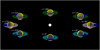 |
Fig. 1 Various illumination and viewing geometries in a planet-ring system simulated with Pryngles. The star (white dot) and planetary orbit are not to scale. The circular planetary orbit has an inclination angle i of 60°. The ring has an inclination angle γ of 70° and a roll angle λr of 0° (this system is thus mirror-symmetric from left to right). The true planetary anomaly ν is shown next to each planet image and increases rotating counterclockwise. The colors of the spangles in this figure are indicative of viewing and illumination conditions, following the conventions explained in the text. |
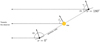 |
Fig. 2 Definition of the angles used to define the orientation of the orbit and ring as projected in a side view of the planet-ring system at the orbital locations in which the true planet anomaly ν is 0° and 180°. |
2.3 Physics of light scattering
The formalism we used has been described in detail in previous works (see eg. Hansen & Travis 1974; Hovenier et al. 2004; Stam & Hovenier 2005; Rossi & Stam 2018). For clarity, we reproduce the definition of the essential quantities that were calculated as part of the results of our numerical experiments.
Unidirectional beams of light are described here using Stokes vectors (Hansen & Travis 1974; Hovenier et al. 2004),
![Mathematical equation: $F \equiv \left[ {\matrix{ F \hfill \cr Q \hfill \cr U \hfill \cr V \hfill \cr } } \right],$](/articles/aa/full_html/2025/01/aa47194-23/aa47194-23-eq1.png) (1)
(1)
with F the total flux, Q and U the linearly polarized fluxes, and V the circularly polarized flux. All these quantities are measured in W m−2 or W m−3 when the wavelength is included. The circularly polarized flux V is usually very low compared to F, Q, and U and was neglected (Rossi & Stam 2018). This does not yield significant errors in the computation of the most significant components F, Q, and U (Stam & Hovenier 2005).
Linearly polarized fluxes Q and U are defined with respect to a reference plane and can be rotated from one reference plane to the next using the rotation matrix L. Neglecting circular polarization, L is given by (see e.g. Hovenier et al. 2004)
![Mathematical equation: $L(\beta ) = \left[ {\matrix{ 1 & 0 & 0 \cr 0 & {\cos 2\beta } & {\sin 2\beta } \cr 0 & { - \sin 2\beta } & {\cos 2\beta } \cr } } \right].$](/articles/aa/full_html/2025/01/aa47194-23/aa47194-23-eq2.png) (2)
(2)
Here, β is the angle between the old and new reference planes, measured in counterclockwise direction when looking toward the observer. A description of the procedure we devised for computing β at each spangle is included in Appendix C.
We also computed the polarized flux Fpol and the degree of polarization P, which are independent of the chosen reference plane and are defined as
 (3)
(3)
and
 (4)
(4)
2.4 Locally reflected and transmitted starlight
To obtain the Stokes vector of light that is reflected/transmitted by the planet-ring system as a whole, we added the contributions of the individual active spangles, that is, those that are visible and illuminated, in a similar fashion as done in Sections 2 and 3 in Zuluaga et al. (2022).
The Stokes vector  that is locally reflected by the nth planetary/ring spangle is calculated as (Hansen & Travis 1974)
 (5)
(5)
where x is either p or r if the spangle belongs to the planet or ring surface, respectively, µ(0)n = cos θ(0)n with θ0 and θ the illumination and observation angles, respectively, and ϕn – ϕ0n is the local azimuthal difference angle (see Appendix C for the definition of these angles).  is the first column of the local reflection matrix, and πF0 is the flux of the incident starlight as measured on a plane perpendicular to the direction of incidence.
We assumed that starlight is unidirectional and unpolarized when integrated over the stellar disk. This assumption is based on the very low disk-integrated polarized fluxes of active and inactive FGK stars (Cotton et al. 2017) and on measurements of the Sun (Kemp et al. 1987). Because of this assumption, we do not need the full reflection matrix in Equation (5), but only its first column.
The Stokes vector for light that is locally diffusely transmitted through the nth ring spangle is calculated using
 (6)
(6)
with  the first column of the local transmission matrix. Since we assumed a flat ring and parallel incident light, every ring spangle had the same illumination µ0 , viewing µ, and azimuthal difference ϕ – ϕ0 angles.
The local reflection and transmission matrices  , and
, and  are a function of the physical properties of the medium they represent. This means that
  depends on the chemical composition and optical thickness of the atmosphere as well as on the surface albedo, while
  and
and  depend on the optical thickness of the ring and the optical properties of the particles in the ring. We assumed that all planetary and ring spangles have the same properties.
Calculating reflection and transmission matrices for all individual values of µ and µ0 across the planet and the ring spangles is prohibitively expensive in computational terms. Instead, the model developed for this work and incorporated in Pryngles uses a method similar to Rossi et al. (2018). Our model uses precalculated coefficients of a Fourier expansion of  , and
, and  obtained for various combinations of µ0 and µ. The coefficients were computed using an adding–doubling radiative transfer algorithm that fully includes polarization and all orders of scattering (see de Haan et al. 1987, for a detailed description of the adding-doubling algorithm and the Fourier series expansion). We used bicubic spline interpolation for values of µ0 and/or µ that fall between the calculated Fourier coefficients. We thoroughly tested the procedure and reproduced well-known results found in the literature before we used the model to study the reflected light of a ringed planet Pryngles2.
2.5 Integrated fluxes and polarization
The Stokes vector of the light that is reflected by the planet(p)- ring(r) system as a whole can be written as
 (7)
(7)
The Stokes vector Fp of the planet can be written as the sum of the local Stokes vectors over the Np active planetary spangles, as follows:
 (8)
(8)
Here, d is the distance to the observer, b is the optical thickness of the ring (see Section 3), Ap is the surface area of a planetary spangle ( , with rp the planetary radius), L(βn) the rotation matrix for the nth spangle (see Equation (2)), and an is a parameter that depends on whether the planetary spangle is in occultation and/or in the shadow of the ring. The four possible values or formulae for calculating an are provided in Table 1.
The local meridian plane is the reference plane for the Stokes parameters Q and U of the nth spangle. This plane contains the normal to the surface and the direction toward the observer. Since they are located on a sphere, different planetary spangles generally have different local meridian planes. Logically, all ring spangles have the same local meridian plane. To add the contribution of all spangles, the matrix L in Equation (8) rotates the local Stokes vector from the local meridian plane of a spangle to the reference plane of the system as a whole, namely to the so-called detector plane (DP). This plane is fixed with respect to the planet and its ring, and it is equivalent to the xz-plane when viewed from the observer reference frame of the original Pryngles (see Zuluaga et al. 2022 for details).
The Stokes vector of the ring, Fr is calculated using
 (9)
(9)
when the ring reflects the incident starlight. In this formula, Nr is the number of active ring spangles. When the ring is seen in transmitted light, the Stokes vector is given by
 (10)
(10)
In the previous expressions, all the ring spangles have the same surface area, Ar . For a circular ring with an outer radius rout and an inner radius rin (measured in planetary radius units rp), the spangle area is defined as  . The area of the ring spangles is not necessarily the same as the area of the planetary spangles.
We normalized the total and polarized fluxes, F and Fpol , computed by summing the contribution of reflected/transmitted starlight from all spangles, such that at a phase angle a of 0o, the total flux F is equal to the ringless planet geometric albedo AG . The fluxes we computed and report in the following sections are thus dimensionless. The actual fluxes received from a given planetary system, measured in W m−2, can be obtained by multiplying the normalized value by the normalization factor Fnorm ,
 (11)
(11)
with πF0 the flux of the starlight that is incident on the planet, rp the radius of the planet, and d the distance between the system and the observer. This normalization was made in order to shrink the parameter space while demonstrating the impact that rings have on the flux and polarization curves.
To test a correct implementation of our formalism, we calculated the total flux reflected by a planet with a Lambertian reflecting surface. In this case, the total reflected flux of a planet at a phase angle α and with a geometric albedo As is given by
![Mathematical equation: $F(\alpha ) = {{2{A_s}} \over {3\pi }}[\sin \alpha + (\pi - \alpha )\cos \alpha ].$](/articles/aa/full_html/2025/01/aa47194-23/aa47194-23-eq27.png) (12)
(12)
In Figure 3, we show the difference between the flux calculated with Pryngles and that calculated using Equation (12). The agreement between our model with the theory is noticeable. This tells us that the formulae and approximations described in this section are properly implemented in the package, and gives us confidence to apply Pryngles to study more complex cases.
Values and formulae of an.
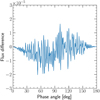 |
Fig. 3 Difference in flux calculated using the analytical phase function of a Lambertian surface and a mock (nonringed) planet with 10 000 spangles. |
3 A test planet and its rings
After improving Pryngles with a more realistic model of light scattering and polarization, we focused on the scientific insights we may gain from applying our model. For this purpose, we designed a series of numerical experiments in which we varied the most important geometrical and physical parameters of the planet and the model. It is important to stress that although these experiments can be seen as simple computational tests of the package, they are mainly intended for and were analyzed to better understand the revealing signatures that rings may produce in the polarimetric light curves of exoplanets.
Our test planet had a perfect spherical shape and a gaseous atmosphere bounded below by a Lambertian reflecting surface with an albedo of 0.5 that mimics a deep cloud layer. The gas molecules in the atmosphere were anisotropic Rayleigh scatter- ers with a depolarization factor of 0.02, which is a typical value to model the scattering properties of H2 (Hansen & Travis 1974).
The planet was surrounded by a flat, circular, and horizontally homogeneous ring. Although we assumed that the ring was infinitely thin, it was composed of irregularly shaped particles with finite sizes. The optical thickness b of our model ring varied between 0.01 and 4.0, which is the range of optical thicknesses at visible wavelengths found across the horizontally inhomogeneous rings of Saturn (Lissauer & de Pater 2019). The single-scattering albedo ϖ and the scattering matrix (Mishchenko 2009) of the ring particles depend on their size, shape, and composition, and for nonspherical particles, on their orientation. Our model ring particles were irregularly shaped and randomly oriented. It is important to use irregularly shaped particles to avoid sharp angular features such as rainbows or glories that arise when using spherical particles (Goloub et al. 2000; Nousiainen et al. 2012).
For our numerical experiments, we only used one type of particle to keep the number of varied parameters down. This is justified because the change in behavior from a spherical particle to an irregular particle is generally much larger than between irregular particles of different composition, provided the size is the same for all three (Nousiainen et al. 2012). This holds especially true when the degree of polarization of the reflected light is computed.
The single-scattering properties of our ring particles are based on laboratory measurements of light scattered by olivine particles of sizes described by a log-normal distribution (Muñoz et al. 2000). The scattering matrix of these particles was calculated by Moreno et al. (2006) using the discrete dipole approximation (DDA) method (Draine & Flatau 1994, 2004) to fit the measurements. The light-scattering measurements are available at 442 and 633 nm. We used the 633 nm data, keeping in mind the wavelength region and capabilities of JWST (Rieke et al. 2005; Jakobsen et al. 2022). We selected particles that Moreno et al. (2006) called “shape 5” particles, with an average projected surface area of 4.2 µm2 and equivalent radii of up to 1 µm to use in our calculations. For use in our adding-doubling radiative transfer algorithm, we expanded the scattering matrix elements of the ring particles into generalized spherical functions (de Rooij & van der Stap 1984).
The chosen particle size meant that the modeled ring was more similar to the E ring of Saturn, which has particle sizes between 0.2 and 10 µm (Ye et al. 2016). Larger macroscopic particles would mean that their mutual shadowing must be considered. This is not needed to illustrate the basic effects of a ring on the reflected flux and degree of polarization of a planet. It would also require a different radiative transfer approach.
The flux F and degree of polarization P of the light that is singly scattered by the ring particles and the gaseous molecules that form the planetary atmosphere are shown in Figure 4. In the measurements by Muñoz et al. (2000), the phase functions were not absolutely calibrated since the number of particles in the aerosol beam in the laboratory experiment is not known. The singly scattered fluxes were normalized such that their average overall scattering directions equal one (Hansen & Travis 1974).
We defined our standard system as a planet with a ring with rin = 1.20 and rout = 2.25 planet radii, which is similar to the radii of the Saturn ring (Lissauer & de Pater 2019). The optical thickness b of the ring was 1.0, and the ring particles had a single-scattering albedo ϖ of 0.8. This high albedo mimics the bright, icy particles in the Saturn ring. Our standard system had i = 20°, λr = 30°, and γ = 60°. The ring-plane crossings in this system occurred at ν = 69.4° and ν = 249.4° (see Equation (A.1) for details). Between these values of ν, the ring is seen in diffusely transmitted starlight, while at lower or higher values of ν, the ring is seen in reflected starlight. Every result we present was solved for the entire orbit using a step size of 1°.
4 Results
4.1 A ringless planet
In order to understand the effect of a ring on the polarimetric light curve of a planet, we first need to know the expected flux of a planet devoid of a ring. Figure 5 shows the reflected flux F, the polarized flux Fpol , and the degree of polarization P of our model ringless planet as functions of the true anomaly ν. Hereafter, we call these three plots the “polarimetric light-curve set”.
We varied orbital inclination angles i ranging from 0° (a face-on orbit) to 90° (edge-on orbit) to study the effect of this parameter on the light curve. In all plots, the total and polarized fluxes were normalized as described in Section 2.5.
The obtained polarimetric light curves with Pryngles are very similar to those calculated with independent methods in Stam et al. (2004); Buenzli & Schmid (2009). This provides a new confirmation of the validity of our models, at least for ringless planets. For i = 0°, the phase angle α is always 90°, and F, Fpol , and P are thus constant along the orbit (solid thick line in Figure 5). For i > 0°, the planet attains its largest phase angle at ν = 0° and 360°, and its smallest one at v = 180°. For an edge-on orbit (i = 90°), the planet is precisely in front of its star at ν = 0° and 360° and thus in transit (dip in the flux plot).
As expected, P is highest around ν = 90° and 270° (see the upper panel of Figure 5) when α ≈ 90° and the single-scattering degree of polarization of the gaseous molecules is highest (see the peaks in the bottom plot of Figure 4). The peak of polarized flux (middle panel in Figure 5) shifts toward ν = 180° at low i because it is not just a function of the degree of polarization of the light, but is also modulated by the flux. The flux (upper panel in Figure 5) increases with decreasing α, that is, with increasing orbital inclination i, because of the biased phase function of molecules toward forward scattering (peak around θ = 0 in Figure 4). The small peaks in P for i = 90° around low and high values of ν are caused by light that has been scattered twice in the atmosphere as described in Stam et al. (2004). The direction of polarization of this twice-scattered light is parallel to the detector plane.
In summary, we showed in this first experiment that our model reproduces known features of the polarimetric light curve of a ringless planet. More importantly for our paper, we have polarimetric light curves against which we can compare our results. This allow us to recognize the effect of rings in polarization in the next numerical experiments.
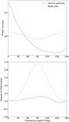 |
Fig. 4 Phase function or flux (top) and degree of polarization (bottom) of incident unpolarized light that has been singly scattered by gas molecules (dashed orange) and the irregularly shaped ring particles (Moreno et al. 2006) (solid blue) as functions of the single-scattering angle Θ (Θ = 0° for forward-scattered light). The fluxes have been normalized such that their average overall scattering directions equal one (Hansen & Travis 1974). Positive (negative) polarization indicates a direction of polarization perpendicular (parallel) to the plane through the incident and scattered-light beams. |
 |
Fig. 5 Polarimetric light-curve set of a ringless planet and its dependence on the orbital inclination angle i. From top to bottom: Normalized total flux F , normalized polarized flux Fpol , and degree of polarization P. |
4.2 Effect of rings on flux and polarization
Figures 6 and 7 summarize the effect of a ring on the polarimetric light curve of a ringed planet and constitute the most important result of this paper. There, we show the influence of the orientation of the ring for two different planetary orbital inclination angles: i = 20° in Figure 6, which may correspond to the case of a planetary system that would have been discovered or studied using direct imaging; and i = 90° in Figure 7, which shows the case of a system discovered or studied using the transit method. As we mentioned in Section 1, we especially focused on the novel results represented by Figure 6 and the observability of exorings around exoplanets found through direct observation.
In the polarimetric light-curve sets (flux, polarized flux, and degree of polarization), one per row at different values of the ring roll angle λr, we include for comparison purposes the corresponding light curve of a ringless planet (solid curve). We discuss important features in the light curves of Figure 6 and Figure 7 and highlight their effect on observability.
4.2.1 The effect of shadows
The most salient features in the light curves are those produced by the changing shadows (see Figure 1). Although we do not discuss all features created in the light curves by shadows in full detail, a few characteristic features are highlighted for the benefit of interpreting future observations. While the phase curves of the planet itself are symmetric around ν = 0°, a nonzero ring inclination longitude λr makes them asymmetric. This was noted before (Arnold & Schneider 2004; Dyudina et al. 2005).
The first interesting and highly nontrivial results are those obtained when the ring is edge-on (γ = 90°, dotted lines in all panels). Since the view on the ring is independent of λr (see the inset planet diagram to the left), the polarimetric light curves for this case are the same in all rows in each figure. Although in this configuration, the observer receives no light reflected by or transmitted through the ring, depending on orbital inclination, the ring does leave traces in the light curves. For example, in Figure 6 for every γ = 90°, the shadow the ring casts on the planet reduces F and Fpol between approximately ν = 50° and 130°, and 230° and 310°. This effect is more noticeable for λr = 90° , when the ring is seen edge-on for all γ. We conclude that a wiggly structure of the polarimetric light curves is a revealing signature of shadows cast on the planet by a ring.
4.2.2 Plane-crossing discontinuities
For all the geometrical configurations, the flux and polarization of the light reflected by ringed exoplanets almost coincide with the ringless case at the ring-plane crossings, that is, where the ring is illuminated at its edge and the shadow is infinitely narrow. For λr = 0° (upper row in the two figures), the ring-plane crossings occur at v = 90° and 270°, but for other values of λr and/or γ (the latter only when λr ≠ 0), the locations of the ringplane crossings are slightly different but easy to identify since the ringed and ringless curves intersect at the crossings.
Ring-plane crossings usually manifest themselves in the light curves as sharp changes in the slope of the curves (e.g., discontinuities in the derivatives of the curve). This effect is due to a change in the light-scattering regime from light that i is reflected before or after the ring-plane crossing to light transmitted through the ring. A prime example of this discontinuity in Figure 6 is when λr = 0° (first row) and γ = 60° (dash-dotted green lines). In this case, between ν = 0° and 90°, the ring reflects the stellar light and produces higher F values than in the ringless case. After the ring-plane crossing, the ring transmits light but also casts a shadow on the planet, which decreases the flux F with respect to the ringless situation. It might be difficult to observe these sharp features, which also occur in Figure 7 because it requires high-cadence observations. Nonetheless, it would be very valuable in characterizing the features for which we search.
4.2.3 Reflection versus transmission
The λr = 0° (first row) and γ = 0° curve (dashed blue line) in Figure 6 aptly demonstrates another interesting effect of rings on reflected light curves. The difference in the behavior with respect to the γ = 60° curve (dashed green lines) arises from the fact that the ring transmits and reflects light in different parts of the orbit. However, in this case, the forward-scattering peak manifests itself as a strong increase in the transmitted light with respect to the ringless case (high peak in the dashed blue line). In summary, even when rings do not reflect light from the star, they may produce intense peaks in the flux via the forward scattering of ring particles.
Another good example of the difference between reflection and transmission is shown in Figure 6 for λr = 30° and λr = 60° (second and third row, respectively). The orientation of the ring causes the light curve to be highly asymmetrical. With peak fluxes around ν = 270°, which in our orbit configuration coincides with the location in the orbit where the angular separation between the star and planet is largest, the observability is higher. Depending on the orientation of the orbital plane, however, this could also hamper observability. The fact that the presence of a ring can shift the location of peak flux during the orbit is an important observation. It is a way of distinguishing ringed planets from nonringed planets.
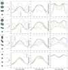 |
Fig. 6 F (left), Fpol (middle), and P (right) of the light that is reflected by the model planet with a Saturn-like ring with rin = 1.2 and rout = 2.25, b = 1.0, and i = 20° (αmin = 70° and αmax = 110°) as functions of the true anomaly v. The ring inclination longitude λr is 0° (first row), 30° (second row), 60° (third row), and 90° (bottom row). For λr = 90° the ring is seen edge-on. The ring inclination angle γ is 0° (dash-dot-dot blue), 30° (long dash green), 60° (long-dash-dot red), or 90° (dot-dot purple). For γ = 90°, there is no dependence on λr. The black lines show the planet without a ring. The images on the left illustrate the planet with its ring at ν = 0°, i.e., when it is closest to the observer. |
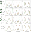 |
Fig. 7 Similar to Fig. 6, except for i = 90°. The images on the left illustrate the system at ν = 0°, which for i = 90° is precisely in front of the star, i.e., the nightside of the planet is turned toward the observer. To keep the structures in the curves visible, we limited the vertical axis in the graphs for F-. In some cases, the forward-scattering peaks are therefore cut off. The missing peak values are the following: for λr = 0°, the lines reach 6.13, 5.37, and 2.25 for γ = 0°, 30°, and 60°, respectively. For λr = 30°, they reach 5.36, 4.61, and 1.55, and for λr = 30°, 2.38 and 1.65 for γ = 0° and γ = 30°, respectively. |
4.2.4 Effects on polarization
Ring-plane crossings appear to be even more pronounced in P than in F and Fpol (third column in Figures 6 and 7). The curves of Fpol clearly show that the light that is reflected by the system in configurations when the ring blocks part of the light that is reflected by the planet is usually less polarized than the light in the ringless case. In some cases, this effect significantly suppresses the degree of polarization P of the light from the system as a whole. This result can be understood by examining Figure 4: the light that is scattered singly by the ring particles not only has a lower P, but at large scattering angles Θ (small planetary phase angles α), it also has an opposite direction of polarization (negative values at the tail of the curve in Figure 4) as compared with the light that is scattered in the planetary atmosphere. This further decreases P of the whole system.
The ring shadow on the planet can slightly increase P when it breaks the symmetry of the illuminated and visible planetary disk. Examples of this effect are evident in the case of γ = 90° (dotted red lines) in Figure 6. In these cases, the edge-on ring prevents light from being reflected on the ring (no polarization effect), but P is slightly larger (smaller) just before (after) the ring-plane crossings due to the break in symmetry. Another good example is the drops in the P curves observed for γ = 60° (dashed-dotted green line) when λr = 0° (first row) and 30° (second row). The drops occur before and after the ring-plane crossings, when the ring casts its shadow on the planet, again breaking the symmetry.
Interpreting the behavior of Fpol is less straightforward. On the one hand, the changes observed in this quantity do not match the changes perceived in the total flux. On the other hand, as explained before, we would expect that the polarized flux is consistently lower when the ring is present. This is not the case, however. For example, in Figure 6, when λr = 30° and λr = 60° (second and third rows), the ring adds some polarized flux during the second half of the orbit (ν > 90°) because although it is weakly polarized, the reflection and forward scattering of light from the huge surface of the ring still adds polarized flux to the total. This effect is also noticeable when i = 90° (Figure 7), where for λr < 90° the polarized flux curves show significant bumps at the beginning and end of the orbit.
4.2.5 Rings on edge-on orbits
The case of an edge-on i = 90° transiting orbit (Figure 7) exhibits interesting differences with respect to that of a nontransiting one. Although most of these features have been discussed by Lietzow & Wolf (2023), our smaller orbital step size (1° vs. 5° in Lietzow & Wolf 2023) leads to sharper features in the light curve than Lietzow & Wolf (2023). Furthermore, we examined a larger selection of ring orientations and found that certain ring orientations lead to more distinct asymmetries.
Comparing Figures 7 to 6, we first of all find that the ring is much brighter in diffusely transmitted light (huge wings at low and high values of ν) than in reflected light (peak around ν ~ 180°). The reason for this behavior is the strong single forward scattering of the ring particles (see Figure 4). At these observing angles, we observe the dark side of the planet, and therefore, the ring dominates the flux from the system. This also explains why the polarization is low in these configurations.
This forward-scattering peak might be expected to be easily detectable. However, since the orbit is edge-on, the angular separation between the planet and its star will be very small and the forward-scattered light will be blended into the stellar light. Still, these peaks might be observable by monitoring the brightness of the star and variations therein. This was demonstrated by Placek et al. (2014) in the infrared, where hot giant planets are relatively bright, but it might also be observed at visible wavelengths, as suggested by Sucerquia et al. (2020).
The second noticeable difference between the transiting and nontransiting case is the structure of the degree of polarization (third column in Figure 7) curves. The dramatic drops in P in the analogous curves of Figure 6 are also present here, but the presence of rings no longer significantly changes the shape of the curves. Instead, the peak P value is often just decreased (see, e.g., the second and third rows). This makes it harder to distinguish the polarization curves of a ringed planet from those of a ringless one.
A ringless planet with clouds might also exhibit similarly oscillating P curves (see Stam et al. 2004; Karalidi et al. 2012) and mimick the effect of rings. However, the asymmetry on the polarization curves, such as those observed for the case of λr = 30° (second row in Figure 7), might help us to identify the revealing signatures of rings. It would have to be ruled out that the asymmetrical behavior is due to seasonal effects on a horizontally inhomogeneous ringless planet, however, as remarked by Dyudina et al. (2005). Even if this were the case, seasonal effects could not explain the sharp changes due to the ring-plane crossings (see, e.g., the features at ν = 300° when λr = 30°).
In order to study the effect that other key physical parameters such as the optical thickness, the single-scattering albedo, and the ring size have on the polarimetric light curves of a ringed planet, we performed a limited but rigorous exploration of the parameter space. We present the results of these explorations in Appendix D.
5 The case of HIP 41378 f
To show the usefulness and potential of Pryngles for the study of future exoring candidates, we performed a numerical exercise on the controversial case of the puffed-up planet HIP 41378 f (Akinsanmi et al. 2020; Alam et al. 2022). We present two general problems (questions) about this case here and use Pryngles to address them. The first problem is to calculate the flux of reflected light on the ring and planet system. This flux would help us to evaluate whether the planet is detectable with available instruments. If it is not, we wish to know the required level of sensitivities for measuring reflected light on planets such as HIP 41378 f. The second problem or question is that if we can measure the light from the planet and its polarization with a temporal resolution that is high enough, how we distinguish the ringless from the ringed planet case using polarimetry. Moreover, we are interested in knowing how polarimetric data could be used to characterize a hypothetical ring around the planet.
HIP 41378 f has a relatively large semimajor orbital axis of about 1.4 AU, which at a distance of 103 pc translates into a sky-projected angular separation with its F-type parent star of ~13 mas (Santerne et al. 2019). This would be large enough to resolve the planet using direct-imaging telescopes such as the proposed Large UV/Optical/Infrared Surveyor (LUVOIR) (The LUVOIR Team 2019) or the Habitable Worlds Observatory (HWO) (National Academies of Sciences, Engineering, and Medicine 2021). The planet has an equilibrium temperature Teq of ~294 K (assuming a bond albedo of zero; Santerne et al. 2019), so that no significant thermal emission would be mixed in the reflected starlight and decrease the degree of polarization of the planet P of the light reflected by the planet. The transit of HIP 41378 f was discovered as part of the K2 mission (Howell et al. 2014), which used visible wavelengths comparable to the 633 nm we used in our previous computations.
HIP 41378 f has an extremely low average density of 0.09 ± 0.02 g cm−3, which is rather unusual according to the available theories of planetary interiors. However, by assuming that a ring partly causes the transit depth, Akinsanmi et al. (2020) reported that a planet with an average density ρp of 1.2 ± 0.4 g cm−3 explains the transit curve slightly better than a low-density ringless planet. A recent follow-up observational study by Alam et al. (2022) showed that the hypothesis of a ring holds when the observations are made over a range of wavelengths. Nonetheless, they did not discard the case of an extended atmosphere either so far. Other possibilities to explain the anomalous low density also include the presence of exomoons (Harada et al. 2023). In summary, although an interesting case, it is too early to consider this as a ringed planet candidate.
In Table 2 we present the parameters of the planet as derived from Akinsanmi et al. (2020). In the table, rp is the planet radius (expressed in Earth radius r⊕), a is the orbital semimajor axis, and r* is the stellar radius. The value of the inclination and roll angle of the ring we provide here are different than those in Akinsanmi et al. (2020) because we defined these angles differently, but they represent the same physical situation.
In order to show the detectability of the reflected light, we used the extremes of the ring optical thickness b and singlescattering albedo ϖ of ring particles that are still compatible with the constraints imposed by the properties of the rings shown in Table 2. ϖ is unconstrained by the transit but can have a significant influence on the reflected flux (see Figure D.3). We used extreme values of ϖ of 0.05 and 0.8. It is worth mentioning, however, that a value of 0.8 seems too high for ring particles that due to the estimated equilibrium temperature are expected to consist of rocky material. However, Akinsanmi et al. (2020) and Alam et al. (2022) estimated an average density ρ of the ring particles of 1.08 ± 0.3 g cm−3, which is low compared to most rocky materials. Explanations for the anomalously low density could be that the particles are porous (Carry 2012) or contain ice deposits from an unknown source.
Akinsanmi et al. (2020) and Alam et al. (2022) assumed a completely opaque ring, which is far from a realistic case. Model simulations of the transit performed with Pryngles showed that using b ≥ 4 results in a transit depth that is fairly close to the observations. Therefore, we varied b between 4 and 20. These values are high enough for an opaque ring, but not unrealistic.
We used the scattering properties of the same olivine particles as in the previous sections since the size of the particles is similar to those assumed by the follow-up study of Alam et al. (2022). Finally, and for the sake of simplicity, we used the same gaseous planetary atmosphere as for our test planet in Section 5. In Figure 8, we show the polarimetric light curves (F, Fpol, and P), assuming a different combination of the free parameters ϖ and b.
Even in the most favorable case, the contrast required to detect the light reflected by the planet is on the order of tens of parts per billion (ppb). Due to the effect of the shadows cast by the ring on the planet, the ringed case could counterintuitively require even lower sensitivities at the level of a few ppb. This is certainly not achievable with SPHERE/ZIMPOL (Thalmann et al. 2008) or with JWST (Carter et al. 2023), especially at the small angular separation for the maximum flux of 13 mas. The following analysis is thus an exercise in what we can learn from a measured light curve in the (near) future.
When the particle albedo is low, only the shadow of the ring on the planet leaves an impression. This means that it will be very hard to detect a ring in any reflected light curve. Only by very accurately measuring the degree of polarization could such a ring be detected. For high-albedo particles, we can more readily distinguish the ringed from the ring-less planet, and we can discern some ring properties.
Based on the flux alone, it is in principle possible to determine the optical thickness of the ring based on the forwardscattering peak. For a certain ring orientation, the reflected flux at ν = 90° is mostly a function of the albedo, while the transmitted flux for low ν is strongly dependent on the optical thickness (see the upper panel in Figure 8). The caveat is that the angular separation is small when the additional flux due to the ring is high. The asymmetrical shape of the flux curve would make it distinguishable from a ringless planet.
The detectability of a ring is further boosted by the fact that the transmitted and reflected light from the ring has a lower degree of polarization. The bottom panel of Figure 8 shows that the albedo and optical thickness might also be constrained by observing the system when ν = 270°, which coincidentally is also when the angular separation is largest. Measuring the degree of polarization when ν = 90° would also allow for the detection of a ring without measuring the forward-scattering peak.
Some considerations are required. Other processes mimic the behavior of a ring. As mentioned in Section 4.2, a planet with seasonal changes might also exhibit asymmetrical light curves (Dyudina et al. 2005). Furthermore, the reflected light of a planet with an exomoon (Harada et al. 2023) might in theory produce anomalous changes in the polarimetric light curves. Since the moon may move in front of the planet, or vice versa, the symmetry breaks would change the polarization of the reflected light. However, the possibility that this would occur during an observation depends on the size and period of the moon and on the observation frequency (Berzosa Molina et al. 2018). Moreover, these mutual transits will result in shallow and brief dips in the polarimetric light curve. These dips could be especially small in polarization (around 2% according to Berzosa Molina et al. 2018) and would mean that the effect of moons would be distinguishable from the effects of a ring.
In summary, although the evidence for the presence of a ring around HIP 41378 f is still marginal, the planet offered us an interesting experimental case for applying the model and tools we implemented in Pryngles. We find that although the reflected light from HIP 41378 f cannot be detected with current instruments, it might be used to reveal the presence of a ring, but only when the polarization can also be measured. For a cadence and sensitivity that are high enough, polarization might even help us to constrain the properties of the ring, such as the composition and optical thickness.
HIP 41378 f parameters (without uncertainties).
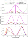 |
Fig. 8 Polarimetric light-curve set of a ringed and ringless HIP 41378 f planet for different values of b and ϖ as functions of ν. The magenta curves pertain to the ringless puffed-up planet, and the black curves show the ringed planet model, but without a ring, using the parameter values of Akinsanmi et al. (2020). All curves use the same orbital inclination and stellar properties, but the magenta curve has a different semimajor axis (a/r* = 231.6). In the Fpol plot, the magenta curve has been omitted as it has the same shape as the black curve, except with maximum values up to 0.0015 ppm. In the P plot, the magenta and black curves overlap. |
6 Discussion
In general, the developments presented here can contribute to three fronts in the search for exoplanets with rings: rings around exoplanets in close-in orbits (i.e., warm exorings), circumplanetary disks (CPDs), and rings around distant giant planets similar to the Saturn rings. Concerning the first case, populations of warm rings that were originally proposed by Schlichting & Chang (2011) can exist in proximity to their host stars for millions of years and are composed of refractory particles rather than icy particles, as the Saturn rings. Although the thermal emission of warm rings cannot be modeled using the current version of our model, it might be added as a constant since thermal emission is predicted to have a relatively low degree of polarization (Stolker et al. 2017). It is important to point out that Pryngles is only designed to calculate the optical properties of cold disks that are infinitely thin. To model more general CPDs requires not only different physics, but probably different computational models. Still, the geometrical machinery of the model is essentially the same.
The second case, that is, massive planets with extensive orbits, has a higher likelihood of developing substantial CPDs, which may ultimately transform into planetary rings upon completion of the satellite formation process. These planet-ring systems might be detected using high-contrast imaging techniques, which are the sole method of planet detection that offers spatial resolution of photons emanating from planets and their surroundings (see, e.g. Ruane et al. 2018). This approach uses coronagraphs or other nulling methods to suppress light from the central star, and in conjunction with observing techniques such as angular differential imaging can attain contrasts of 10−6 at separations of tenths of arcseconds (Marois et al. 2010).
Consequently, this method enables the detection of self- luminous gas giants (i.e., planets that are still forming) on wide orbits and the effects of their presumed rings. To date, planets identified using direct imaging are generally a few million years old and situated tens of astronomical units from their host star. This favors the survival of icy rings. High-contrast imaging has yielded several significant discoveries, including the detection of four planets orbiting HR 8799 (Marois et al. 2010) and the planet β Pic b (Lagrange et al. 2010). As a result, the advancements presented in this paper demonstrate a potential for modeling the CPD populations discovered through the aforementioned techniques.
The third case, that is, rings that are similar to the Saturn rings, was studied in this paper. The study of light scattered from planetary rings around exoplanets is highly relevant to the current search for Saturn-like planets, and their characterization can reveal important information about their evolution and their environments. The modeling of the scattering and polarization of dust grains in planetary rings can provide valuable insights into the composition and evolution of the rings themselves, as well as into the dynamics of the planet-ring system as a whole. Unfortunately, our numerical predictions can currently not be validated through actual observations of Saturn because ground-based telescopes (or space telescopes in the vicinity of Earth) can only observe these planets at small phase angles, where the degree of polarization of the reflected light is very low because of a symmetric geometry. Observing these planets as if they were exoplanets is only possible with orbiters, such as the Cassini spacecraft, or with a flyby mission. However, although the Cassini Imaging Science Subsystem instrument had polarimetric capabilities (Porco et al. 2004), no polarimetric observations of Saturn and its ring system have been published so far (West 2022, priv. comm.).
While the particles we used have a more realistic scattering behavior than similarly sized spherical particles, they were comprised of material that is not typically found in a ring. For example, the rings of Saturn are mainly composed of icy materials (Cuzzi et al. 1984) and have a different refractive index compared to the olivine particles that we used here. To remedy this shortcoming, future package updates will add different ring particles based on data in the Amsterdam-Granada database (Muñoz et al. 2012). Another potential problem is that the used particles have a log-normal distribution (Muñoz et al. 2000; Moreno et al. 2006) while ring particles have a power-law distribution (Dohnanyi 1969; Cuzzi & Pollack 1978). The difference in scattering behavior of the two different size distributions should be investigated in a future study. The effect of inhomogeneous rings should also be explored in the future as our model ring is horizontally homogeneous, while real planetary rings, such as those in the Solar System, are not. Radial variations in the optical thickness and particle properties of our Solar System ring are widespread, and some also exhibit azimuthal variations. These inhomogeneities influence the ring shadows and occultations, and their traces in the signals of planet-ring systems would be interesting to explore.
Although Pryngles can handle eccentric orbits, we assumed circular orbits to reduce the number of free parameters. Our results can be scaled for eccentric orbits by multiplying the total and polarized fluxes by a factor to represent the actual incident fluxes on the planet and its ring (the degree of polarization of the reflected signal would not be affected by the orbital eccentricity). A potential complexity with simulating a ringed planet in a significantly eccentric orbit is that depending on the size of the rings and the semimajor axis of the orbit, the illumination angle might no longer be uniform for the ring, while we assumed a single illumination angle in the ring3.
Although each of the varied system parameters has distinct effects on the light curve, we demonstrated that they also overlap. Especially the properties of the ring, such as optical thickness, particle albedo, and size, show some degenerate behavior. Properties such as the size of the ring and its optical thickness also affect the stability of the ring, which might aid in narrowing down the parameter space to obtain a singular fit. This fit should include eccentric orbits, which is already possible using Pryngles, and different planetary atmospheres, as was done by Lietzow & Wolf (2023), which is not yet possible with the package. The variation in the latter is interesting to combine with observations in different wavelength bands, in particular, at wavelengths in which the gases in the planetary atmosphere absorb and where the planet is thus dark, which could highlight the presence of rings and help us to characterize them.
7 Summary and conclusions
We computed the effects of a ring around an extrasolar planet on the total and polarized fluxes of starlight reflected by the system. For these computations, we extended the novel photometry Python package Pryngles with an adding-doubling radiative transfer algorithm that included all orders of scattering and polarization. We studied the case of hypothetical planets with a similar radius as Saturn, surrounded by dusty rings that are comprised of irregularly shaped particles with an effective radius of 1 µm. By varying the system parameters (orbital and ring inclination, ring roll angle, optical thickness, particle single albedo, and ring size), we investigated how the polarimetric light curve of the system is affected by the presence of a ring. To further illustrate the application of our model and tools to the case of a real planet, we calculated the polarimetric light curves of HIP 41378 f, assuming it has a ring, as hypothesized in some papers (Akinsanmi et al. 2020; Alam et al. 2022).
Our results revealed a number of features in the polarimetric light curves that would be indicative of a ring. Some of these features have been identified in previous works, but others have been overlooked. In general, the light curve of a planet with a ring (total flux as a function of true anomaly) has two peaks, one peak due to the light reflected on the planet and the ring, and the other peak due to the diffusely transmitted light. This behavior was predicted by Arnold & Schneider (2004) and Dyudina et al. (2005).
When we included polarization, however, we were able to identify that the second flux peak also has a substantially lower degree of polarization. This effect arises from differences between the way in which the molecules in the atmosphere of the planet and ring particles polarize the light. This dichotomy between a higher flux but a lower degree of polarization is therefore a key signature of a ring. This was also reported in a recent study by Lietzow & Wolf (2023).
The experimental case study we performed on HIP 41378 f showed that it is currently impossible to directly observe such a system. It might be observable with the next generation of space telescopes, such as LUVOIR (The LUVOIR Team 2019), HabEx (Gaudi et al. 2020), or the recently announced Habitable Worlds Observatory (HabWorlds or HWO) by NASA (National Academies of Sciences, Engineering, and Medicine 2021). Our results suggest that it would indeed be very beneficial for these missions to use polarimetry because it allows the identification of properties such as the optical thickness and particle albedo of exorings. This is not possible using flux measurements alone.
Polarimetry might also be valuable as a method for detecting and characterizing the magnetic fields of ringed exoplanets. As in the case of the giant planets in the Solar System (and in the debris disks around young stars), a planetary magnetic field can modify the optical properties of the rings by influencing the particle orientations (Dollfus 1984; Lazarian 2007). Finding ring-particle orientations could thus potentially provide valuable information about the structure and dynamics of the planet interior, which in turn could provide clues about the habitability of these worlds (in the case of rocky planets) and their satellites (see, e.g., Heller & Zuluaga 2013).
Acknowledgements
We appreciate the comments and suggestions of an anonymous reviewer. JIZ is supported by Minciencias Grant 1115-852-70719/70939. MS acknowledges support from ANID (Agencia Nacional de Investigación y Desarrollo) through FONDECYT postdoctoral 3210605. This project was supported by the European Research Council (ERC) under the European Union Horizon Europe research and innovation program (grant agreement No. 101042275, project Stellar-MADE).
Appendix A Calculating the ring-plane crossings
The location of the ring-plane crossings can be calculated by
 (A.1)
(A.1)
with nr the normal vector to the ring, νrp the true anomaly of the ring-plane crossings and nstar the normal vector pointing from the planet to the star.
We may express these locations in terms of the key orientation angles introduced in Section 2.2:
![Mathematical equation: $\matrix{ {\sin \left( {{\lambda _{\rm{r}}}} \right)\cos (\gamma )\sin \left( {{v_{rp}}} \right) + } & {} \cr {} & {\quad \cos \left( {{v_{rp}}} \right)\left[ {\cos \left( {{\lambda _{\rm{r}}}} \right)\cos (\gamma )\sin (i) - \sin (\gamma )\cos (i)} \right] = 0.} \cr } $](/articles/aa/full_html/2025/01/aa47194-23/aa47194-23-eq29.png)
For example, if we have a system with an orbital inclination i = 20°, and a ring with a roll angle λr = 30°, and inclination γ = 60°, the solution of the previous equation predicts that the ring-plane crossings will happen at ν = 69.4° and ν = 249.4°.
Appendix B The geometry of spangle light-scattering
In Section 2.5 for computing the integrated flux reflected or scattered on the ring and planet spangles, we need to know the angles of the incoming and outcoming light rays, These angles determine the values of parameters µ and ф in Equations (8)-(10). We schematically illustrate in Figure B.1 how these angles are defined.
For each spangle, we define the local stellar zenith angle θ0 as the angle between the local zenith direction and the direction towards the star. Analogously the local viewing zenith angle θ, is the angle between the local zenith direction and the direction towards the observer. From them, we define the local azimuthal difference angle ф − ф0, taken as the angle between the plane that contains the direction towards the local zenith and the direction towards the observer, and the plane that contains the direction towards the local zenith and the direction of propagation of the incident starlight. It is important to stress that the angle ф − ф0 is measured rotating in the clockwise direction when looking towards the local zenith (see de Haan et al. 1987). For a description of our computation of ф − ф0 , see the next section.
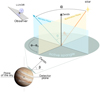 |
Fig. B.1 Spangle geometry: orientation and angles involved in the calculation of stellar light scattering by an individual spangle, along with the observer’s orientation (here, a LUVOIR-type telescope is the observer). |
In all cases, we assume that the incident direction of the starlight is the same across the planet and the ring (the local incident angles depend of course on the spangle). This assumption would not hold for computations for planets with very wide rings and/or that are very close (≪ 0.1 AU) to their star.
B.1 Spangle states
Given the orientation angles i, γ, and λr (which are part of the user-provided input to the package), Pryngles computes, for each true anomaly ν along the planetary orbit, the phase angle α, and for each spangle on the planet and the ring, the angles θ0 , θ, and ф − ф0 . Unlike the planet spangles, all ring spangles have the same illumination and viewing geometries at a given value of ν. Then, taking into account the radius of the planet, the inner and outer radii of the ring, and the direction to the star, Pryngles computes the state of the spangle, namely, whether it is illuminated by the star and visible to the observer; whether it is in the shadow of the ring (for planet-spangles) or the planet (for ring-spangles); and/or whether it is occulted by the ring (for planet-spangles) or the planet (for ring-spangles) (for a discussion on the key concept of “spangle state” in Pryngles, see the original paper by Zuluaga et al. 2022).
Appendix C Computing ф − ф0 and β
The most critical calculation with Pryngles depends on the knowledge we have of the azimuth difference (ф − ф0) and the angle β between the reference and the detector plane at each spangle (see Section 2.5).
The azimuthal angles (ф and ф0 ) are defined with respect to any plane containing the local z-axis. This makes the plane that also contains the observer an obvious choice since it eliminates one of the two angles that need to be calculated, namely ф. Thus an expression is needed for ф0 which then automatically also becomes an expression for ф − ф0 .
Using the spherical law of cosine an expression can be found for an intermediate angle we name δ which is used to find ф0 with respect to the plane containing the direction to the observer and local z-axis (see Figure C.1),
 (C.1)
(C.1)
 (C.2)
(C.2)
where the subscript i stands for the ith spangle.
Care has to be taken, however, to make sure the angle that is found using the above equation is for a rotation that is clockwise when looking in the positive local zenith direction. Whether the found angle needs to be adjusted depends generally on the orientation of the spangle, be it planetary or ring, and the direction of the star-light. The dependency on the location of the star can be understood from Figure C.1 where α will change during the orbit, eventually moving to the other side of the plane formed by ûi and ûobs, the normal vector of the spangle and the normal vector pointing to the observer respectively.
For planetary spangles, the angles are modified as
 (C.3)
(C.3)
 (C.4)
(C.4)
with  the y-location of the spangle with respect to the planetary scattering plane. Here, the criterion is to compensate for the flipping of the normal vector for spangles on the “southern” hemisphere. The dependency on the location of the star is already incorporated into the y-location with respect to the planetary scattering plane.
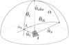 |
Fig. C.1 The angles and unit vectors associated with each individual spangle i. They are: the phase angle α, direction to observer ûobs, direction to the star ûs, normal vector ûi, illumination angle θi,0, viewing angle θi, azimuthal angle ф0,i, and intermediate angle δi. The rotation angle βi is not shown here. |
Since all ring spangles have the same normal vector there is no dependency on their location on the ring. There is, however, a dependency on the orientation of the ring since it determines the locations in the orbit where the flip in the rotation direction happens. The locations of these flips are defined as the place where the plane containing the star, the planet, and the observer and the plane containing the normal vector of the ring and the observer are parallel. A 2D projection of the problem is shown in Figure C.2 with the two vectors in the direction of the star ûstar, (1,2) representing two moments in the orbit.
Two situations arise, depending on the orientation of the ring. If the normal vector of the ring ûring is pointing in the +y direction,
 (C.5)
(C.5)
when the vector pointing to the star ûstar is on the −x side of the plane formed by ûring and the observer. If ûring is pointing in the −y direction,
 (C.6)
(C.6)
when ûstar is on the +x side of the plane formed by that same plane.
The angle between the local meridian plane and the detector plane, β, is also calculated differently for ring spangles compared to planetary spangles. For planetary spangles, the angle is only dependent on their location on the planet. With the detector plane as the reference plane, β is calculated as
 (C.7)
(C.7)
 (C.8)
(C.8)
where the coordinates (xi, yi) are in the observer reference frame. The addition of π is there to make sure the angle that is calculated rotates in the correct direction.
Because all ring spangles have the same normal vector the rotation angle does not depend on the location of the individual spangles. Using the spherical cosine law we can find an equation that instead depends on the orientation of the ring
 (C.9)
(C.9)
 (C.10)
with σ = arctan2 the angle the normal vector makes with the x-axis and
  the z-component of the normal vector. Again the condition of
  is added to make sure the rotation direction stays the same.
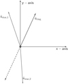 |
Fig. C.2 Illustration of the condition for changing the calculation of β, described in the text. |
Appendix D Exploring the parameter space
After exploring the effect that changing the geometrical configuration of the orbit and the ring has in the polarimetric light curve, we will study in this appendix the impact that other key parameters have on the flux and polarization of the light reflected in our test ringed planet.
In particular, we will focus on three parameters: ring optical thickness (b), single-scattering albedo of ring particles (ϖ), and ring size (ri, re).
D.1 The influence of the ring optical thickness
In Figure D.1 we show the influence of the ring optical thickness b on the polarimetric light curve of the standard planet-ring system, in a particular orbital and ring configuration (namely i = 20°, λr = 30°, γ = 60°). First, we want to discuss the influence of b along the part of the orbit where the ring reflects incident light, and then the more complicated part where the ring diffusely transmits light.
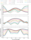 |
Fig. D.1 F (top), Fpol (middle), and P (bottom) as functions of ν for ring optical thicknesses b ranging from 0.01 (dark blue) to 4.0 (brown). For this planet-ring system, i = 20°, λr = 30°, γ = 60°, rin = 1.20, rout = 2.25, and ϖ = 0.8. The black line represents the ringless planet. |
In the figure, the ring reflects light for ν ≤ 69.4° or ≥ 249.4°. In those segments of the orbit the flux F increases as a whole. The increase in F increases with b, although not linearly. With increasing b, the increase in F vanishes as the reflection by the ring reaches an asymptotic value when increasing b does not further increase F. Note that along this part of the orbit, the planet also casts its shadow on the ring, thus decreasing the ring contribution to F, while the ring hardly casts a shadow on the planet.
In reflected light, polarized flux Fpol of the system is lower than that of the ringless planet (solid black curve) at small values of ν and vice-versa. The reason for the lower and higher values of Fpol when the ring is added is due to the polarized flux of the light that is singly scattered by the ring particles, which has an opposite direction of that of the gas molecules in the planet atmosphere at the small values of ν, where the single-scattering angle θ is larger than 150°, and the same direction at the large values of ν, where θ is smaller than 150° (see Figure 4).
Between 69.4° < ν < 249.4°, the ring diffusely transmits light, adding light to the total flux of the system. At the same time, the ring casts shadows on the planetary disk and occults part of it; both effects act at suppressing the planetary flux (see Figure 1).
To understand the relation between the transmitted light and b, in Figure D.2 we show F, Fpol, and P of diffusely transmitted light of just a slab of ring-material for a viewing angle of θ = 0°, different angles of incidence θ0 and as functions of b. As can be seen, the curves for F increase with b due to increased scattering of light by the ring particles (the flux of the directly, thus nonscattered beam of light decreases with increasing b), until about b = 1 to 3 (depending on θ0 and θ as those angles affect the effective ring optical thickness). Further increases of b decrease the diffusely transmitted F as fewer and fewer photons get through the ring.
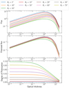 |
Fig. D.2 The diffusely transmitted F (top), Fpol (middle), and P (bottom) as functions of the optical thickness b of a slab of ring-material for illumination angles θ0 ranging from 0° (blue) to 80° (green). The viewing angle θ is 0°. |
The relatively large values of F between ν ≈ 100° and 210° in Figure D.1, are due to the changing size of the planet shadow on the ring. Similar behavior can be seen for Fpol .
The degree of polarization P generally decreases with increasing b as the amount of multiple scattered, generally low polarized, light, increases with b. Between ν = 69.4° and 249.4° where the flux of the reflected ring light is small, this depolarizing effect is not very prominent, especially not for b = 4.0: the very small ring-flux hardly contributes to F and Fpol while at the same time, the ring strongly shadows and occults the planet and thus also decreases the total flux of the system.
D.2 The influence of the single-scattering albedo
Now we will vary the single-scattering albedo ϖ of the ring particles. The variation of these parameters will be equivalent to varying different particle compositions. Icy particles surrounding Saturn would, for example, not survive at the distance between the Earth and the Sun, therefore it would be important to also look at refractory materials (which have a lower albedo in the visible) (Piironen et al. 1998; Ostrowski & Bryson 2019).
In Figure D.3 we show the polarimetric light curves for the standard planet-ring system, with the same geometrical parameters used in the previous section, but with a variable ϖ ranging from 0.05 to 0.8.
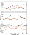 |
Fig. D.3 Similar to Fig. D.1, except for different single-scattering albedos ϖ of the ring particles: 0.05 (blue, dashed), 0.3 (orange, dashed- dot-dot), 0.5 (green, dotted), and 0.8 (red, short-dashed-dotted). The system-parameters are i = 20°, λr = 30°, γ = 60°, rin = 1.20, rout = 2.25, and b = 1.0. |
Not surprisingly, increasing ϖ increases the total flux F, regardless of whether the ring is seen in reflected or transmitted light. Because for a given b, ϖ has no effect on the shadowing or occultation by the ring, and because the single-scattering polarization of the particles is independent of ϖ, Fpol shows little dependence on ϖ, indirectly showing how small the contribution of the ring is to Fpol of the system. The variation in P is thus mostly due to the variation in F.
By comparing Figure D.1 and Figure D.3, we conclude that for this system, it is difficult to determine whether a curve would be due to a larger value of b or a higher value of ϖ. Increases in either parameter lead to higher fluxes when the ring is reflecting light and a larger b can also increase the transmitted flux. For a different orientation of the ring and/or planetary orbit, this might be different. A full retrieval algorithm to fit the physical and geometrical parameters may break the degeneration.
D.3 The influence of the ring radius
The effect that the ring radius rout has on the polarimetric light curves is shown in Figure D.4. The curves are very similar to those for various ring optical thicknesses b (see Figure D.1) since increasing rout increases the reflected fluxes and, depending on the geometry, also the size of shadows, in a similar way as increasing b does. There are some key differences, however. For example, along parts of the orbit where the ring is diffusely transmitting light, the ring flux increases with increasing rout while it would decrease with increasing b beyond a value of about 1.0 (see Figure D.2).
Another difference compared to changing b is found in the curves for Fpol: while increasing b decreases Fpol of the system as a whole, because light that has been scattered multiple times is less polarized, there is no such relation with the ring size: the larger rout, the larger the Fpol that is added to the signal of the planet-ring system.
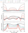 |
Fig. D.4 Similar to Fig. D.1, except for different outer ring radii rout (expressed in planet-radius r): 1.75 (blue), 2.0 (green), 2.25 (purple), 2.5 (pink), 3.0 (orange), 4.0 (red), and 5.0 (brown). The system-parameters are i = 20°, λ = 30°, γ = 60°, rin = 1.2, w = 0.8, and b = 1.0. |
With increasing rout, the curves for P converge as the polarization signal of the rings starts to dominate that of the planet (except near the ring-plane crossings). This trend is helped by the fact that eventually, increasing rout no longer increases the extent of the shadows on the planet.
The dips around ν = 15° and 290° become more pronounced when the ring brightens as is evident from Figure D.1, Figure D.3, and Figure D.4. At these locations in the orbit, the angle of polarization of the ring light is opposite to that of the planet light, thus decreasing P; an effect that becomes more prominent with increasing rout. For rout = 5.0, the flux that is reflected by the ring dominates the planetary flux and P no longer approaches zero.
References
- Akinsanmi, B., Santos, N. C., Faria, J. P., et al. 2020, A&A, 635, L8 [NASA ADS] [CrossRef] [EDP Sciences] [Google Scholar]
- Alam, M. K., Kirk, J., Dressing, C. D., et al. 2022, ApJ, 927, L5 [NASA ADS] [CrossRef] [Google Scholar]
- Arnold, L., & Schneider, J. 2004, A&A, 420, 1153 [NASA ADS] [CrossRef] [EDP Sciences] [Google Scholar]
- Berzosa Molina, J., Rossi, L., & Stam, D. M. 2018, A&A, 618, A162 [NASA ADS] [CrossRef] [EDP Sciences] [Google Scholar]
- Buenzli, E., & Schmid, H. M. 2009, A&A, 504, 259 [NASA ADS] [CrossRef] [EDP Sciences] [Google Scholar]
- Carry, B. 2012, Planet. Space Sci., 73, 98 [CrossRef] [Google Scholar]
- Carter, A. L., Hinkley, S., Kammerer, J., et al. 2023, ApJ, 951, L20 [NASA ADS] [CrossRef] [Google Scholar]
- Charnoz, S., Canup, R. M., Crida, A., & Dones, L. 2018, in Planetary Ring Systems. Properties, Structure, and Evolution, eds. M. S. Tiscareno, & C. D. Murray, 517 [CrossRef] [Google Scholar]
- Cotton, D. V., Marshall, J. P., Bailey, J., et al. 2017, MNRAS, 467, 873 [NASA ADS] [Google Scholar]
- Cuzzi, J. N., & Pollack, J. B. 1978, Icarus, 33, 233 [NASA ADS] [CrossRef] [Google Scholar]
- Cuzzi, J. N., Lissauer, J. J., Esposito, L. W., et al. 1984, in IAU Colloq. 75: Planetary Rings, eds. R. Greenberg, & A. Brahic, 73 [Google Scholar]
- de Haan, J. F., Bosma, P. B., & Hovenier, J. W. 1987, A&A, 183, 371 [Google Scholar]
- de Rooij, W. A., & van der Stap, C. C. A. H. 1984, A&A, 131, 237 [Google Scholar]
- Demory, B. O., Sulis, S., Meier Valdés, E., et al. 2023, A&A, 669, A64 [NASA ADS] [CrossRef] [EDP Sciences] [Google Scholar]
- Dohnanyi, J. S. 1969, J. Geophys. Res., 74, 2531 [Google Scholar]
- Dollfus, A. 1984, in Planetary Rings, ed. A. Brahic, 121 [Google Scholar]
- Draine, B. T., & Flatau, P. J. 1994, J. Opt. Soc. Am. A, 11, 1491 [NASA ADS] [CrossRef] [Google Scholar]
- Draine, B. T., & Flatau, P. J. 2004, arXiv e-prints [arXiv:astro-ph/0409262] [Google Scholar]
- Dyudina, U. A., Sackett, P. D., Bayliss, D. D. R., et al. 2005, ApJ, 618, 973 [NASA ADS] [CrossRef] [Google Scholar]
- Gaudi, B. S., Seager, S., Mennesson, B., et al. 2020, arXiv e-prints [arXiv:2001.06683] [Google Scholar]
- Goloub, P., Herman, M., Chepfer, H., et al. 2000, J. Geophys. Res., 105, 14 747 [Google Scholar]
- Hansen, J. E., & Travis, L. D. 1974, Space Sci. Rev., 16, 527 [Google Scholar]
- Harada, C. K., Dressing, C. D., Alam, M. K., et al. 2023, AJ, 166, 208 [NASA ADS] [CrossRef] [Google Scholar]
- Heller, R., & Zuluaga, J. I. 2013, ApJ, 776, L33 [NASA ADS] [CrossRef] [Google Scholar]
- Hovenier, J. W., Van Der Mee, C., & Domke, H. 2004, Transfer of Polarized Light in Planetary Atmospheres: Basic Concepts and Practical Methods, 318 (Springer Science & Business Media) [Google Scholar]
- Howell, S. B., Sobeck, C., Haas, M., et al. 2014, PASP, 126, 398 [Google Scholar]
- Jakobsen, P., Ferruit, P., Alves de Oliveira, C., et al. 2022, A&A, 661, A80 [NASA ADS] [CrossRef] [EDP Sciences] [Google Scholar]
- Karalidi, T., Stam, D. M., & Hovenier, J. W. 2012, A&A, 548, A90 [NASA ADS] [CrossRef] [EDP Sciences] [Google Scholar]
- Karalidi, T., Stam, D. M., & Guirado, D. 2013, A&A, 555, A127 [NASA ADS] [CrossRef] [EDP Sciences] [Google Scholar]
- Kemp, J. C., Henson, G. D., Steiner, C. T., & Powell, E. R. 1987, Nature, 326, 270 [NASA ADS] [CrossRef] [Google Scholar]
- Knutson, H. A., Charbonneau, D., Allen, L. E., et al. 2007, Nature, 447, 183 [NASA ADS] [CrossRef] [Google Scholar]
- Lagrange, A. M., Bonnefoy, M., Chauvin, G., et al. 2010, Science, 329, 57 [Google Scholar]
- Lazarian, A. 2007, J. Quant. Spec. Radiat. Transf., 106, 225 [NASA ADS] [CrossRef] [Google Scholar]
- Lietzow, M., & Wolf, S. 2023, A&A, 671, A113 [NASA ADS] [CrossRef] [EDP Sciences] [Google Scholar]
- Lissauer, J. J., & de Pater, I. 2019, Fundamental Planetary Science, updated Edn. (Cambridge University Press) [CrossRef] [Google Scholar]
- Marois, C., Zuckerman, B., Konopacky, Q. M., Macintosh, B., & Barman, T. 2010, Nature, 468, 1080 [NASA ADS] [CrossRef] [Google Scholar]
- Meier Valdés, E. A., Morris, B. M., Wells, R. D., Schanche, N., & Demory, B.-O. 2022, A&A, 663, A95 [NASA ADS] [CrossRef] [EDP Sciences] [Google Scholar]
- Mishchenko, M. I. 2009, J. Quant. Spec. Radiat. Transf., 110, 808 [NASA ADS] [CrossRef] [Google Scholar]
- Moreno, F., Vilaplana, R., Muñoz, O., Molina, A., & Guirado, D. 2006, J. Quant. Spec. Radiat. Transf., 100, 277 [NASA ADS] [CrossRef] [Google Scholar]
- Morris, B. M., Delrez, L., Brandeker, A., et al. 2021, A&A, 653, A173 [NASA ADS] [CrossRef] [EDP Sciences] [Google Scholar]
- Muñoz, O., Volten, H., de Haan, J. F., Vassen, W., & Hovenier, J. W. 2000, A&A, 360, 777 [Google Scholar]
- Muñoz, O., Moreno, F., Guirado, D., et al. 2012, J. Quant. Spec. Radiat. Transf., 113, 565 [CrossRef] [Google Scholar]
- National Academies of Sciences, Engineering, and Medicine 2021, Pathways to Discovery in Astronomy and Astrophysics for the 2020s [Google Scholar]
- Nousiainen, T., Zubko, E., Lindqvist, H., Kahnert, M., & Tyynelä, J. 2012, J. Quant. Spec. Radiat. Transf., 113, 2391 [NASA ADS] [CrossRef] [Google Scholar]
- Ohno, K., & Fortney, J. J. 2022, ApJ, 930, 50 [NASA ADS] [CrossRef] [Google Scholar]
- Ostrowski, D., & Bryson, K. 2019, Planet. Space Sci., 165, 148 [NASA ADS] [CrossRef] [Google Scholar]
- Piironen, J., Muinonen, K., Nousiainen, T., et al. 1998, Planet. Space Sci., 46, 937 [NASA ADS] [CrossRef] [Google Scholar]
- Piro, A. L., & Vissapragada, S. 2020, AJ, 159, 131 [CrossRef] [Google Scholar]
- Placek, B., Knuth, K. H., & Angerhausen, D. 2014, ApJ, 795, 112 [NASA ADS] [CrossRef] [Google Scholar]
- Porco, C. C., West, R. A., Squyres, S., et al. 2004, Space Sci. Rev., 115, 363 [NASA ADS] [CrossRef] [Google Scholar]
- Porco, C. C., Weiss, J. W., Richardson, D. C., et al. 2008, AJ, 136, 2172 [NASA ADS] [CrossRef] [Google Scholar]
- Rieke, M. J., Kelly, D., & Horner, S. 2005, SPIE Conf. Ser., 5904, 1 [NASA ADS] [Google Scholar]
- Rossi, L., & Stam, D. M. 2018, A&A, 616, A117 [NASA ADS] [CrossRef] [EDP Sciences] [Google Scholar]
- Rossi, L., Berzosa-Molina, J., & Stam, D. M. 2018, A&A, 616, A147 [NASA ADS] [CrossRef] [EDP Sciences] [Google Scholar]
- Ruane, G., Riggs, A., Mazoyer, J., et al. 2018, SPIE Conf. Ser., 10698, 106982S [NASA ADS] [Google Scholar]
- Santerne, A., Malavolta, L., Kosiarek, M. R., et al. 2019, arXiv e-prints [arXiv:1911.07355] [Google Scholar]
- Schlichting, H. E., & Chang, P. 2011, ApJ, 734, 117 [NASA ADS] [CrossRef] [Google Scholar]
- Schmid, H. M., Bazzon, A., Roelfsema, R., et al. 2018, A&A, 619, A9 [NASA ADS] [CrossRef] [EDP Sciences] [Google Scholar]
- Stam, D. M., & Hovenier, J. W. 2005, A&A, 444, 275 [NASA ADS] [CrossRef] [EDP Sciences] [Google Scholar]
- Stam, D. M., Hovenier, J. W., & Waters, L. B. F. M. 2004, A&A, 428, 663 [NASA ADS] [CrossRef] [EDP Sciences] [Google Scholar]
- Stolker, T., Min, M., Stam, D. M., et al. 2017, A&A, 607, A42 [NASA ADS] [CrossRef] [EDP Sciences] [Google Scholar]
- Sucerquia, M., Alvarado-Montes, J. A., Zuluaga, J. I., Montesinos, M., & Bayo, A. 2020, MNRAS, 496, L85 [NASA ADS] [CrossRef] [Google Scholar]
- Tamburo, P., Mandell, A., Deming, D., & Garhart, E. 2018, AJ, 155, 221 [NASA ADS] [CrossRef] [Google Scholar]
- Thalmann, C., Schmid, H. M., Boccaletti, A., et al. 2008, SPIE Conf. Ser., 7014, 70143F [NASA ADS] [Google Scholar]
- The LUVOIR Team 2019, arXiv e-prints [arXiv:1912.06219] [Google Scholar]
- Ye, S. Y., Gurnett, D. A., & Kurth, W. S. 2016, Icarus, 279, 51 [NASA ADS] [CrossRef] [Google Scholar]
- Zuluaga, J. I., Kipping, D. M., Sucerquia, M., & Alvarado, J. A. 2015, ApJ, 803, L14 [NASA ADS] [CrossRef] [Google Scholar]
- Zuluaga, J. I., Sucerquia, M., & Alvarado-Montes, J. A. 2022, Astron. Comput., 40, 100623 [NASA ADS] [CrossRef] [Google Scholar]
ASCL entry available at https://ascl.net/2205.016. Package PyPI repository available at https://pypi.org/project/pryngles
The results of these tests are available in the notebooks published together with the latest version of Pryngles in the GitHub public repository of the package https://github.com/seap-udea/pryngles-public
Pryngles itself can handle different illumination angles for different ring spangles, but we did not consider this in this paper.
All Tables
All Figures
|
Fig. 1 Various illumination and viewing geometries in a planet-ring system simulated with Pryngles. The star (white dot) and planetary orbit are not to scale. The circular planetary orbit has an inclination angle i of 60°. The ring has an inclination angle γ of 70° and a roll angle λr of 0° (this system is thus mirror-symmetric from left to right). The true planetary anomaly ν is shown next to each planet image and increases rotating counterclockwise. The colors of the spangles in this figure are indicative of viewing and illumination conditions, following the conventions explained in the text. |
| In the text | |
|
Fig. 2 Definition of the angles used to define the orientation of the orbit and ring as projected in a side view of the planet-ring system at the orbital locations in which the true planet anomaly ν is 0° and 180°. |
| In the text | |
|
Fig. 3 Difference in flux calculated using the analytical phase function of a Lambertian surface and a mock (nonringed) planet with 10 000 spangles. |
| In the text | |
|
Fig. 4 Phase function or flux (top) and degree of polarization (bottom) of incident unpolarized light that has been singly scattered by gas molecules (dashed orange) and the irregularly shaped ring particles (Moreno et al. 2006) (solid blue) as functions of the single-scattering angle Θ (Θ = 0° for forward-scattered light). The fluxes have been normalized such that their average overall scattering directions equal one (Hansen & Travis 1974). Positive (negative) polarization indicates a direction of polarization perpendicular (parallel) to the plane through the incident and scattered-light beams. |
| In the text | |
|
Fig. 5 Polarimetric light-curve set of a ringless planet and its dependence on the orbital inclination angle i. From top to bottom: Normalized total flux F , normalized polarized flux Fpol , and degree of polarization P. |
| In the text | |
|
Fig. 6 F (left), Fpol (middle), and P (right) of the light that is reflected by the model planet with a Saturn-like ring with rin = 1.2 and rout = 2.25, b = 1.0, and i = 20° (αmin = 70° and αmax = 110°) as functions of the true anomaly v. The ring inclination longitude λr is 0° (first row), 30° (second row), 60° (third row), and 90° (bottom row). For λr = 90° the ring is seen edge-on. The ring inclination angle γ is 0° (dash-dot-dot blue), 30° (long dash green), 60° (long-dash-dot red), or 90° (dot-dot purple). For γ = 90°, there is no dependence on λr. The black lines show the planet without a ring. The images on the left illustrate the planet with its ring at ν = 0°, i.e., when it is closest to the observer. |
| In the text | |
|
Fig. 7 Similar to Fig. 6, except for i = 90°. The images on the left illustrate the system at ν = 0°, which for i = 90° is precisely in front of the star, i.e., the nightside of the planet is turned toward the observer. To keep the structures in the curves visible, we limited the vertical axis in the graphs for F-. In some cases, the forward-scattering peaks are therefore cut off. The missing peak values are the following: for λr = 0°, the lines reach 6.13, 5.37, and 2.25 for γ = 0°, 30°, and 60°, respectively. For λr = 30°, they reach 5.36, 4.61, and 1.55, and for λr = 30°, 2.38 and 1.65 for γ = 0° and γ = 30°, respectively. |
| In the text | |
|
Fig. 8 Polarimetric light-curve set of a ringed and ringless HIP 41378 f planet for different values of b and ϖ as functions of ν. The magenta curves pertain to the ringless puffed-up planet, and the black curves show the ringed planet model, but without a ring, using the parameter values of Akinsanmi et al. (2020). All curves use the same orbital inclination and stellar properties, but the magenta curve has a different semimajor axis (a/r* = 231.6). In the Fpol plot, the magenta curve has been omitted as it has the same shape as the black curve, except with maximum values up to 0.0015 ppm. In the P plot, the magenta and black curves overlap. |
| In the text | |
|
Fig. B.1 Spangle geometry: orientation and angles involved in the calculation of stellar light scattering by an individual spangle, along with the observer’s orientation (here, a LUVOIR-type telescope is the observer). |
| In the text | |
|
Fig. C.1 The angles and unit vectors associated with each individual spangle i. They are: the phase angle α, direction to observer ûobs, direction to the star ûs, normal vector ûi, illumination angle θi,0, viewing angle θi, azimuthal angle ф0,i, and intermediate angle δi. The rotation angle βi is not shown here. |
| In the text | |
|
Fig. C.2 Illustration of the condition for changing the calculation of β, described in the text. |
| In the text | |
|
Fig. D.1 F (top), Fpol (middle), and P (bottom) as functions of ν for ring optical thicknesses b ranging from 0.01 (dark blue) to 4.0 (brown). For this planet-ring system, i = 20°, λr = 30°, γ = 60°, rin = 1.20, rout = 2.25, and ϖ = 0.8. The black line represents the ringless planet. |
| In the text | |
|
Fig. D.2 The diffusely transmitted F (top), Fpol (middle), and P (bottom) as functions of the optical thickness b of a slab of ring-material for illumination angles θ0 ranging from 0° (blue) to 80° (green). The viewing angle θ is 0°. |
| In the text | |
|
Fig. D.3 Similar to Fig. D.1, except for different single-scattering albedos ϖ of the ring particles: 0.05 (blue, dashed), 0.3 (orange, dashed- dot-dot), 0.5 (green, dotted), and 0.8 (red, short-dashed-dotted). The system-parameters are i = 20°, λr = 30°, γ = 60°, rin = 1.20, rout = 2.25, and b = 1.0. |
| In the text | |
|
Fig. D.4 Similar to Fig. D.1, except for different outer ring radii rout (expressed in planet-radius r): 1.75 (blue), 2.0 (green), 2.25 (purple), 2.5 (pink), 3.0 (orange), 4.0 (red), and 5.0 (brown). The system-parameters are i = 20°, λ = 30°, γ = 60°, rin = 1.2, w = 0.8, and b = 1.0. |
| In the text | |
Current usage metrics show cumulative count of Article Views (full-text article views including HTML views, PDF and ePub downloads, according to the available data) and Abstracts Views on Vision4Press platform.
Data correspond to usage on the plateform after 2015. The current usage metrics is available 48-96 hours after online publication and is updated daily on week days.
Initial download of the metrics may take a while.