| Issue |
A&A
Volume 692, December 2024
|
|
|---|---|---|
| Article Number | L5 | |
| Number of page(s) | 13 | |
| Section | Letters to the Editor | |
| DOI | https://doi.org/10.1051/0004-6361/202452402 | |
| Published online | 04 December 2024 | |
Letter to the Editor
Forbidden emission line spectro-imaging of the RU Lupi jet and low-velocity component⋆
1
Department of Physics, Maynooth University, Maynooth, Co. Kildare, Ireland
2
Univ. Grenoble Alpes, CNRS, IPAG, 38000 Grenoble, France
3
Lunar and Planetary Laboratory, The University of Arizona, Tucson, AZ 85721, USA
4
Academica Sinica, Institute of Astronomy and Astrophysics, No 1. Sec. 4, Roosevelt Rd., Taipei 10617, Taiwan, ROC
5
Centre for Star and Planet Formation, Globe Institute, University of Copenhagen, Øster Voldgade 5-7, 1350 Copenhagen, Denmark
6
Max-Planck-Institut für Astronomie, Königstuhl 17, 69117 Heidelberg, Germany
7
School of Physics, University College Dublin, Dublin, Ireland
⋆⋆ Corresponding author; This email address is being protected from spambots. You need JavaScript enabled to view it.
Received:
27
September
2024
Accepted:
21
November
2024
Abstract
The first images of the jet and low-velocity component (LVC) from the strongly accreting classical T Tauri star RU Lupi are presented. Adaptive optics-assisted spectro-imaging of forbidden emission lines was used. The main aim of the observations was to test the conclusion from a recent spectro-astrometric study that the narrow component (NC) of the LVC traces a magnetohydrodynamic (MHD) disk wind, and to estimate the mass-loss rate in the wind. The structure and morphology support a wind origin for the NC. The upper limit to the launch radius and semi-opening angle of the wind in [O I] λ6300 emission are estimated to be 2 au and 19°, in agreement with MHD wind models for high accretors. The height of the [O I] λ6300 wind-emitting region, a key parameter for the derivation of the mass-loss rate, is estimated for the first time at ∼35 au, giving Ṁout = 2.6 × 10⁻¹¹ M⊙ yr−1. When compared to the derived mass-accretion rate of Ṁacc = 1.6 × 10⁻⁷ M⊙ yr−1, the efficiency in the wind is too low for the wind to contribute significantly to the angular momentum removal.
Key words: stars: formation / stars: jets / stars: low-mass / stars: individual: RU Lupi / stars: winds / outflows
Based on data obtained from the ESO Science Archive Facility.
© The Authors 2024
 Open Access article, published by EDP Sciences, under the terms of the Creative Commons Attribution License (https://creativecommons.org/licenses/by/4.0), which permits unrestricted use, distribution, and reproduction in any medium, provided the original work is properly cited.
This article is published in open access under the Subscribe to Open model. This email address is being protected from spambots. You need JavaScript enabled to view it. to support open access publication.
1. Introduction
Classical T Tauri stars (CTTSs) are young, low-mass stars in the earliest stages of forming planets and thus are analogues of the early evolution of our Solar System (Ray et al. 2007). A key step in learning how young stars accrete mass and how their disks evolve and form planets is to clarify how angular momentum is lost (Pascucci et al. 2023). Outflows play a critical role here, as CTTSs drive outflows in the form of collimated jets and surrounding winds (e.g. Arulanantham et al. 2024; Bajaj et al. 2024). Magnetohydrodynamic (MHD) winds are strongly favoured as the main mechanism by which angular momentum is removed from the accretion disk, thus regulating accretion (Lesur 2021; Pascucci et al. 2023). The jet is likely the fast inner part of the MHD wind that has been collimated by the magnetic field and accelerated to velocities of > 100 km s−1 (Frank et al. 2014). Photoevaporative (PE) winds produced by energetic radiation (UV and X-ray) from the central star heating the disk are also present, and they are critical to disk dispersal (Ercolano & Pascucci 2017). Current work is focused on identifying direct tracers of MHD winds to test for their presence and their ability to remove angular momentum and regulate accretion.
The low-velocity component (LVC; v < 40 km s−1) of optical forbidden emission lines (FELs) found in the spectra of CTTSs has long been a strong candidate for an MHD wind tracer (Kwan & Tademaru 1988). As the [O I] λ6300 line is the brightest FEL1 most frequently showing an LVC and very often, a high-velocity component (HVC; v > 40 km s−1), it is considered a touchstone for the LVC. The FEL HVC originates from the jet, with the emission region typically extended to several hundred au (Hirth et al. 1997). In contrast, the LVC is spatially compact, which limits what it can reveal about MHD winds (Fang et al. 2023). A further complication is that the LVC likely also traces the PE wind (Rab et al. 2023). To uncover the origin of the LVC, studies have focused on kinematics (Banzatti et al. 2019; Nisini et al. 2024) and spectro-astrometry (Whelan et al. 2021, 2023). The high velocities of the LVC coupled with emission within the potential well of the star revealed by these studies cannot easily be explained by PE winds (Pascucci et al. 2023). Adaptive optics (AO) – assisted integral field spectroscopy (IFS), such as can be done with the Multi Unit Spectroscopic Explorer (MUSE), has the capability to spatially resolve the LVC, allowing its width and height to be measured (Fang et al. 2023; Flores-Rivera et al. 2023). The width provides an upper limit of the launch radius of the outflow, and the height is required to estimate the mass-outflow rate. In combination with the mass-accretion rate, this is a direct test of its contribution to angular momentum removal (Whelan et al. 2021). Therefore, MUSE observations could potentially distinguish between the different origins for the LVC and verify whether MHD winds regulate accretion.
In this Letter, MUSE narrow-field mode (NFM) observations of the jet and wind of the CTTS RU Lupi (d ∼ 140 pc) are presented. The outflow from RU Lupi has previously been investigated with high-resolution spectroscopy and spectro-astrometry, making it an intriguing source to test which additional insights IFS can provide (Takami et al. 2001; Whelan et al. 2021). Spectro-astrometry records the spatial centroids emission as a function of velocity and therefore gives the minimum extent of the outflow, but provides no information on the width and collimation. The [O I] λ6300 and [S II] λ6731 FELs of RU Lupi were shown to have three distinct velocity components (Banzatti et al. 2019). Whelan et al. (2021) classified these components as an HVC with a peak velocity vp ∼ 200 km s−1 (HVC2; hereafter referred to as the jet), a second, intermediate HVC that they suggested was the base of the jet (HVC1; vp = 60 − 100 km s−1) and an LVC narrow component (NC) (vp = 13 − 24 km s−1, hereafter referred to as the NC). The spectro-astrometric analysis of Whelan et al. (2021) using the Ultraviolet and Visual Echelle Spectrograph (UVES) data, revealed three new pieces of information about the RU Lupi NC that were interpreted as it tracing an MHD wind. They were the position angle (PA) that matches the PA of the jet, an emitting region within 2 au of the star, and a negative velocity gradient with offset from the star. The MUSE observations now described offer the first images of the RU Lupi jet and NC along with measurements of their width and height.
2. Observations and data analysis
RU Lupi was observed with MUSE in NFM during July and August 2021 as part of two separate programmes (106.21EN.001 and 0104.C-0919(B)). Both sets of data were accessed through the ESO archive and produced similar results. The 106.21EN.001 data are discussed here as they were found to be of better quality due to the MUSE-DEEP data collection, where the individual observations were aligned and combined to form an observation with a higher signal-to-noise ratio (S/N)2. MUSE covers a spectral range of 4650–9300 Å with a resolving power of R: 2000–4000 (Bacon et al. 2010). The AO provided an angular resolution of 0 074 with a spatial sampling of 0
 025 pixel−1 over a field of view (FOV) of 7
 5 × 7
5 × 7 5. The seeing of the observation is 0
 45. The data were pre-reduced using the ESO MUSE data reduction pipeline. The first step in searching for spatially resolved jet emission was to perform continuum subtraction in the jet-tracing emission lines. This was performed locally around each emission line of interest by subtracting a polynomial fit to the continuum emission from every spatial pixel in the datacube. Outflow emission was identified in the [S II] λ6731 line (Fig. 1). Spatial profiles perpendicular to the jet axis were extracted at numerous positions along the jet and were fit with Gaussian profiles to measure the centroid of the spatial profiles, which are indicative of the jet axis position. In this way, the PA of the jet was accurately measured at 213° ± 2°, which is perpendicular, within the uncertainty of the observations, to the estimated disk PA of 121° ± 5° (Huang et al. 2018). RU Lupi has an almost face-on accretion disk with θi = 19 ° ± 2° (Huang et al. 2018). The continuum-subtracted datacube was rotated so that the PA of 213° lay along the horizontal to facilitate the analysis of the extended emission (Sect. 3.2).
 |
Fig. 1. Integrated (vrad = 270 − 325 km s−1) [S II] λ6731 continuum-subtracted image of the RU Lupi jet with a sector of the ALMA 1.3 mm dust continuum disk image shown in white contours (Andrews et al. 2018). The ALMA beam size (3.5 × 3.4 au) is shown in the lower left corner. The red arrow delineates the disk PA and radius from Huang et al. (2018) (121° ± 5°, 63 ± 1 au), and the dashed green line shows the jet PA measured here (213° ± 2°). The jet and outer knot are perpendicular to the disk, but the inner bright region of the jet at < 50 au from the source is asymmetric about the green line. |
3. Results
The MUSE spectrum of RU Lupi is rich in emission lines tracing accretion and outflow activity (Sect. A). The outflow is identified in the [O I] λ6300, [S II] λλ6716,6731, and [N II] λ6583 lines, and only the jet is detected in [N II] λ6583 (Hirth et al. 1997). Faint emission at all wavelengths is found to fill the field, pointing to the presence of emission scattered from the almost face-on accretion disk. Line to continuum ratio plots were prepared to investigate the nature of the scattered emission (see Sect. B).
3.1. Morphology of the outflow components
Figure 1 shows an [S II] λ6731 image of the jet integrated over the velocity range of 270 km s−1 to –325 km s−1. Close to the source, the outflow is wide and bright. It culminates in a knot at ∼85 au (250 au deprojected). An asymmetry across the jet axis is apparent, as the north-western side is brighter than the south-eastern side. Figure 2 presents continuum-subtracted channel maps of the jet, HVC1, and NC. A Lucy-Richardson deconvolution was performed using continuum point spread functions (PSFs) extracted from spectral regions close to the emission lines3. Due to the decreased spectral resolution of MUSE compared to UVES, the three outflow velocity components are not fully resolved, and any conclusions made from these channel maps should consider this. Morphological differences are present, however. In the highest-velocity channel, a small-scale jet culminating in the shock feature at ∼85 au is seen. As the [N II] λ6583 emission traces only the jet, a clear image of the jet without contamination from the other components is obtained. The morphology of the jet in [N II] λ6583 emission is wide at the base. Faint redshifted emission along the jet PA is seen in [S II] λ6731 at a higher velocity than in the blueshifted jet. This knot is seen at a distance where the dust disk would no longer block the redshifted flow and could be redshifted outflow emission. The velocity of this emission points to a kinematical asymmetry between the two jet lobes. The HVC1 and NC are less extended and wider than the jet, but they are extended beyond the continuum image. This suggests layering in the outflow. The asymmetry across the outflow is also visible in these images and especially in the [S II] λ6731 NC image.
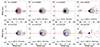 |
Fig. 2. Deconvolved channel maps of the jet, HVC1, and NC emission from RU Lupi in the [O I] λ6300, [S II] λ6731 and [N II] λ6583 emission lines. The distances are not deprojected, and the red box shows the region for which the outflow widths are mapped (Fig. 3). The source position is marked with a blue star. The contour levels begin at 3σ of the background emission and increase by factors of 1.5. |
3.2. Structure of the RU Lupi outflows
Position-velocity diagrams transverse to the outflow axis were prepared from slices extracted at different distances along the outflow (Fig. D.1). Initially, two velocity components are present: The jet, which is seen at all distances, and the NC, which fades with increasing distance from the star. This shows that the NC is a separate outflow component to the jet (see Sect. D). To better understand the structure of the outflow, the spatial widths of the [O I] λ6300, [S II] λ6731 and [N II] λ6583 lines were mapped with distance from the source (Fig. 3). This was achieved by extracting transverse spatial profiles from the channel maps before deconvolution, and by measuring the FWHM and centroids (Fig. G.1) using a Gaussian fitting (Murphy et al. 2021; Kirwan et al. 2022). Measurements were made for the inner portion of the outflow4 marked by the red box in Fig. 2. The angular resolution was subtracted in quadrature from the measured widths to recover the intrinsic width. Measurements below the FWHM of the source PSF were excluded. Halving the lower bounds of the FWHM measurements indicates an upper limit of the radial distance along the disk from which the flows are launched (Table 1). The full opening angle of the outflow is a measure of the degree of collimation of the flow, with the jet expected to be most collimated (Table 1). For the jet, the angle between the straight line fit to the width and the y-intercept of the fit is a lower limit of the full opening angle, with the upper limit being the angle between the straight line fit through the origin. As the width of the NC is larger, especially in the case of the [S II] λ6731 line, the angle between the straight line fit to the width and the y-intercept likely underestimates the opening angle of the NC. We used the angle between a straight line fit through the y-intercept of the jet component as a reasonable estimate of the upper limit of the NC opening angle.
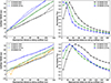 |
Fig. 3. Full width at half maximum (left panels) and normalised flux (right panels) measurements of the jet, HVC1, and NC in [O I] λ6300, [S II] λ6731 and [N II] λ6583 emission, measured along the outflow, with the driving source position at the origin. The error bars on the FWHM data points are the uncertainty of the FWHM in the Gaussian fitting routine, which appear small here due to the high S/N of the transverse spatial profiles. In the right panels, the jet emission follows a different pattern than the HVC1 and NC, indicating an unresolved knot in the jet. The wind height is measured as the width of the NC emission at half the peak flux. |
Launch radii and full opening angles (θ) of the jet and NC.
3.3. Efficiency of the outflow components
The mass-accretion rate of RU Lupi was estimated using the method of Alcalá et al. (2017) and a mass and radius of 0.55 M⊙ and 2.48 R⊙. The accretion luminosities and corresponding mass-accretion rates for the accretion tracers used are given in Table F.1. Some thought had to be given to the optimum aperture size for the extraction of the accretion spectrum (see Sect. E). The mean value of the accretion rate measured is Ṁacc = 1.6 × 10⁻⁷ M⊙ yr−1. Fang et al. (2018) reported a value of  M⊙ yr−1 using a different set of emission lines, and Wendeborn et al. (2024) reported a value of ∼1 × 10⁻⁷ M⊙ yr−1 using accretion shock modelling, flow modelling, and the method of Alcalá et al. (2017), all with LHα, and mitigating the effect of wind absorption, which allowed Hα to be a more reliable accretion tracer. Using the method described by Fang et al. (2018), the mass-outflow rate is estimated to be Ṁout = 2.6 × 10⁻¹¹ M⊙ yr−1 for the [O I] λ6300 NC. This method uses the velocity peak of the NC, the height of the NC emission region, and the luminosity of the NC emission. The low spectral resolution of MUSE poses a challenge here for the measurement of the NC peak velocity and luminosity. Therefore, values from Whelan et al. (2021) and Fang et al. (2018) were used in the calculation, namely v = −4 km s−1 and LOI6300 = 9.54 × 10⁻⁶ L⊙. While Whelan et al. (2021) noted variability in the jet component of the RU Lupi outflow, the NC is seen to remain stable with time. To estimate the height of the NC, a plot of the normalised flux of the outflow components along the jet axis was produced (Fig. 3). The [O I] λ6300 wind height is estimated to be 35 au from Fig. 3, as the width of the NC at half the height of the flux peak. This calculation assumed a temperature of 5000 K and gives a ratio of the mass outflow to accretion rate of ∼0.02%. Taking a temperature of 10 000 K decreases this ratio by an order of magnitude, but a gas temperature of this magnitude is unlikely for the slow-moving NC. For the jet in [O I] λ6300, the method described in Fang et al. (2018) was adopted. LOI6300 = 7.43 × 10⁻⁵ L⊙ was measured from the MUSE data and LOI6300 = 9.77 × 10⁻⁵ L⊙ was taken from Fang et al. (2018). The RU Lupi HVC is known to be variable (Whelan et al. 2021). Using the luminosity from the MUSE data, a tangential jet velocity of –52 km s−1, and l⊥ = 98 au, we found Ṁout = 3.6 × 10⁻⁹ M⊙ yr−1. This increased to Ṁout = 4.7 × 10⁻⁹ M⊙ yr−1 using LOI6300 from Fang et al. (2018). The gas temperature was assumed to be 10 000 K in this calculation, as appropriate for the base of the T-Tauri jets (e.g. Agra-Amboage et al. 2011). The velocity estimate comes from Fang et al. (2018), and the jet height is the projected size of the jet within the extraction aperture. The resulting outflow efficiency is in the range 2.3–2.9%, which is expected for jets (Ray et al. 2007).
4. Discussion
The full opening angle of the jet (Table 1) is large, ∼21° to 28°, compared to other studies, which measured typical opening angles of < 5° (e.g. Murphy et al. 2021). Wide opening angles of jets have been seen in some cases, however (e.g. Pascucci et al. 2024). Blending between the jet and the other outflow velocity components is ruled out as the cause, as the opening angle is also large in [N II] λ6583 emission, which only traces the jet. The jet width measurements could be impacted by the presence of a jet knot. Figure 3 shows a peak in jet brightness at ∼25 au in [O I] λ6300 and ∼45 au in [S II] λ6731 which could be an unresolved shock feature at this distance, with the difference in the peak position in [O I] λ6300 and [S II] λ6731 reflecting the different critical densities the lines. The wide-angled morphology at the base of the jet may also arise from emission scattered off some V-shaped cavity carved into the surrounding ambient medium by the outflow. As the line-to-continuum ratio maps (Fig. B.1) of the high-velocity emission also display this wide-angled morphology, we can rule out contribution from continuum light scattered off a cavity. However, we cannot dismiss the possibility that the spatial distribution of scattered jet emission differs from that of scattered continuum light, resulting in the cavity being illuminated entirely by jet emission. Conversely, the morphology of this wide-angled emission in the jet images does not match what is expected for a cavity of an almost face-on inclination (Whitney et al. 2003).
The opening angles of the NC are smaller than what has been predicted for winds by other studies. Banzatti et al. (2019) showed that the LVC broad component (BC) and NC kinematics correlate, and that blueshifted velocities are maximised at a viewing angle of ∼35°. This was taken as evidence of a conical wind geometry with a half-opening angle of 35°, matching the predictions for conical-shell MHD winds made by Kurosawa & Romanova (2012). However, their models, which give a half-opening angle of 35°, are made for sources with a moderate mass-accretion rate (taken to be 4 × 10⁻⁸ M⊙ yr−1). Kurosawa & Romanova (2012) showed that smaller opening angles are achieved in cases of high accretion, taken to be 3.4 × 10⁻⁷ M⊙ yr−1, comparable to what we measure for RU Lupi. The outflow displays a nested structure, with the jet, traced in [O I] λ6300 and [S II] λ6731, being more collimated and at a higher velocity than the NC, which is wider, moves more slowly, and is launched at larger disk radii. The NC as traced by [S II] λ6731 emission is wider than the [O I] λ6300 emission, again due to the difference in the critical line densities.
Using IFS, we estimated the height of the outflow much better than it can be estimated using spectro-astrometry, which only provides a minimum offset from the source position. This allows a more accurate estimation of Ṁout. However, large uncertainties (Table F.1) remain a challenge when estimating Ṁacc and Ṁout values using line luminosities. Although varying the spectral extraction aperture size when measuring the mass-accretion rate in Sect. E can result in a difference of an order of magnitude, we can be relatively confident in our chosen aperture size and consequently, in our estimated Ṁacc, as the value agrees with values in previous studies that used different accretion tracers and different methods to estimate Ṁacc (e.g. Fang et al. 2018; Wendeborn et al. 2024). We would like to emphasise that the aperture size used in spectral extraction is an important factor to consider when using IFS data to estimate Ṁacc and Ṁout.
5. Summary and conclusions
The MUSE NFM observations presented here provide new insights into the RU Lupi jet and NC. They build on what was previously learned from spectro-astrometry and support the conclusion that the [S II] λ6731 and [O I] λ6300 NC traces an MHD wind. Our main conclusions are summarised as follows.
-
The jet was imaged for the first time in the [O I] λ6300, [S II] λ6731, and [N II] λ6583 forbidden emission lines. It displays a wide full-opening angle (∼21° to 28°) and culminates in a knot at ∼85 au (250 au deprojected), with a spectacular spatial resolution of 0
 74. The opening angle of the jet is large compared to other studies (typically < 5°), but the jet width measurements could be impacted by the presence of an unresolved knot in the inner outflow region or by jet emission scattered off a V-shaped cavity. It is possible that the jet possesses a kinematical asymmetry when the high-velocity redshifted emission detected in [S II] λ6731 is considered.
 -
The jet extends to double the minimum distance suggested by the spectro-astrometric analysis, and its PA (213° ± 2°) is perpendicular to the RU Lupi disk PA (121° ± 5°) within the uncertainties.
-
The outflow efficiency of the jet is at a few percent, which is in line with the values derived for other CTTSs (Ray et al. 2007). The outflow efficiency in the [O I] λ6300 NC is very low, even when all the uncertainties in the calculations are considered, such as poorly understood wind geometries, spatial extents, and contribution to emission from the disk surface (Nisini et al. 2024). The mass-loss rate value places the efficiency of the outflow component that is traced by the NC at < 0.1%, while models suggest that Ṁout ∼ Ṁacc for the wind if it dominates angular momentum removal (Bai 2017). The measured mass-loss rate is also relatively low for PE winds (Pascucci et al. 2023).
-
The opening angles for the NC are smaller than what has been predicted for winds by other studies (∼70°). However, narrower opening angles are predicted in cases of high accretors such as RU Lupi.
-
The NC was also imaged for the first time, allowing its height in [O I] λ6300 to be estimated. The value of ∼35 au measured from Fig. 3 is higher than the 8 au from the [O I] λ6300 spectro-astrometry, which provides a minimum offset. The NC is wider than the jet in [O I] λ6300 and [S II] λ6731, with the [S II] λ6731 emission being wider than the [O I] λ6300 emission due to the difference in the critical line densities. This nested velocity structure supports the wind origin for the NC.
The key result is that the mass-loss rate is significantly lower in the [O I] λ6300 NC than in the jet. Pascucci et al. (2023) argued that with high accretors such as RU Lupi, the wind is predominantly molecular, meaning that atomic wind tracers such as [O I] do not trace the bulk of the wind mass-outflow rate and instead provide a lower limit on Ṁout. For RU Lupi, Pontoppidan et al. (2011) reported that the CO fundamental line at ∼4.7 μm traces a wind, and they estimated Ṁout of the CO wind at 4 × 10⁻⁹ M⊙ yr−1, which is two orders of magnitude higher than the [O I] λ6300 NC. This supports the explanation for the low [O I] λ6300 NC mass-loss rate offered by Pascucci et al. (2023), but the efficiency of the CO outflow is comparable to the FEL jet (∼2%), which means that the CO wind does not dominate angular momentum removal either. This work strongly highlighted the power of IFS for advancing our understanding of the best MHD wind tracer and whether they should be considered important to angular momentum removal in forming stars. VLT/ERIS observations of RU Lupi would be a logical next step as the molecular wind in H2 emission could be analysed in the same way as was done here for [O I] λ6300 and with an improved spectral resolution.
This is due to the large abundance of oxygen and the favourable excitation conditions in the gas.
The 0104.C-0919 (B) data are discussed further in Sect. H.
More details on the PSFs and deconvolution are given in Sect. C.
Beyond this region, the profiles were not well fit by a Gaussian.
Acknowledgments
Work supported by the John & Pat Hume Doctoral Scholarship at Maynooth University (MU) and the Travelling Doctoral Studentship from the National University of Ireland (NUI). We would also like to thank Carlo Manara and Andrea Banzatti for their insightful discussions. A. M. acknowledges the grant from the National Science and Technology Council (NSTC) of Taiwan 112-2112-M-001-031- and 113-2112-M-001-009-. L. Flores-Rivera acknowledges support from the ERC Starting Grant 101041466-EXODOSS.
References
- Agra-Amboage, V., Dougados, C., Cabrit, S., & Reunanen, J. 2011, A&A, 532, A59 [NASA ADS] [CrossRef] [EDP Sciences] [Google Scholar]
- Alcalá, J. M., Manara, C. F., Natta, A., et al. 2017, A&A, 600, A20 [NASA ADS] [CrossRef] [EDP Sciences] [Google Scholar]
- Andrews, S. M., Huang, J., Pérez, L. M., et al. 2018, ApJ, 869, L41 [NASA ADS] [CrossRef] [Google Scholar]
- Arulanantham, N., McClure, M. K., Pontoppidan, K., et al. 2024, ApJ, 965, L13 [NASA ADS] [CrossRef] [Google Scholar]
- Bacon, R., Accardo, M., Adjali, L., et al. 2010, Proc. SPIE, 7735, 773508 [Google Scholar]
- Bai, X.-N. 2017, ApJ, 845, 75 [NASA ADS] [CrossRef] [Google Scholar]
- Bajaj, N. S., Pascucci, I., Gorti, U., et al. 2024, AJ, 167, 127 [NASA ADS] [CrossRef] [Google Scholar]
- Banzatti, A., Pascucci, I., Edwards, S., et al. 2019, ApJ, 870, 76 [Google Scholar]
- Birney, M., Dougados, C., Whelan, E. T., et al. 2024, A&A, in press, https://doi.org/10.1051/0004-6361/202451433 [NASA ADS] [CrossRef] [EDP Sciences] [Google Scholar]
- Delabrosse, V., Dougados, C., Cabrit, S., et al. 2024, A&A, 688, A173 [NASA ADS] [CrossRef] [EDP Sciences] [Google Scholar]
- Ercolano, B., & Pascucci, I. 2017, R. Soc. Open Sci., 4, 170114 [Google Scholar]
- Fang, M., Pascucci, I., Edwards, S., et al. 2018, ApJ, 868, 28 [NASA ADS] [CrossRef] [Google Scholar]
- Fang, M., Wang, L., Herczeg, G. J., et al. 2023, Nat. Astron, 7, 905 [NASA ADS] [CrossRef] [Google Scholar]
- Flores-Rivera, L., Flock, M., Kurtovic, N. T., et al. 2023, A&A, 670, A126 [NASA ADS] [CrossRef] [EDP Sciences] [Google Scholar]
- Frank, A., Ray, T. P., Cabrit, S., et al. 2014, in Protostars and Planets VI, eds. H. Beuther, R. S. Klessen, C. P. Dullemond, & T. Henning, 451 [Google Scholar]
- Hirth, G. A., Mundt, R., & Solf, J. 1997, A&AS, 126, 437 [NASA ADS] [CrossRef] [EDP Sciences] [Google Scholar]
- Huang, J., Andrews, S. M., Dullemond, C. P., et al. 2018, ApJ, 869, L42 [NASA ADS] [CrossRef] [Google Scholar]
- Kirwan, A., Murphy, A., Schneider, P. C., et al. 2022, A&A, 663, A30 [NASA ADS] [CrossRef] [EDP Sciences] [Google Scholar]
- Kurosawa, R., & Romanova, M. M. 2012, MNRAS, 426, 2901 [NASA ADS] [CrossRef] [Google Scholar]
- Kwan, J., & Tademaru, E. 1988, ApJ, 332, L41 [NASA ADS] [CrossRef] [Google Scholar]
- Lesur, G. 2021, J. Plasma Phys., 87, 205870101 [CrossRef] [Google Scholar]
- Murphy, A., Dougados, C., Whelan, E. T., et al. 2021, A&A, 652, A119 [NASA ADS] [CrossRef] [EDP Sciences] [Google Scholar]
- Nisini, B., Gangi, M., Giannini, T., et al. 2024, A&A, 683, A116 [NASA ADS] [CrossRef] [EDP Sciences] [Google Scholar]
- Pascucci, I., Cabrit, S., Edwards, S., et al. 2023, in Protostars and Planets VII, eds. S. Inutsuka, Y. Aikawa, T. Muto, K. Tomida, & M. Tamura, 567 [Google Scholar]
- Pascucci, I., Beck, T. L., Cabrit, S., et al. 2024, Nat. Astron, 1 [Google Scholar]
- Pontoppidan, K. M., Blake, G. A., & Smette, A. 2011, ApJ, 733, 84 [Google Scholar]
- Rab, C., Weber, M. L., Picogna, G., Ercolano, B., & Owen, J. E. 2023, ApJ, 955, L11 [NASA ADS] [CrossRef] [Google Scholar]
- Ray, T., Dougados, C., Bacciotti, F., Eislöffel, J., & Chrysostomou, A. 2007, in Protostars and Planets V, eds. B. Reipurth, D. Jewitt, & K. Keil, 231 [Google Scholar]
- Takami, M., Bailey, J., Gledhill, T. M., Chrysostomou, A., & Hough, J. H. 2001, MNRAS, 323, 177 [NASA ADS] [CrossRef] [Google Scholar]
- Wendeborn, J., Espaillat, C. C., Thanathibodee, T., et al. 2024, ApJ, 972, 100 [NASA ADS] [CrossRef] [Google Scholar]
- Whelan, E. T., Pascucci, I., Gorti, U., et al. 2021, ApJ, 913, 43 [NASA ADS] [CrossRef] [Google Scholar]
- Whelan, E. T., Murphy, A., & Pascucci, I. 2023, ApJ, 951, 1 [CrossRef] [Google Scholar]
- Whitney, B. A., Wood, K., Bjorkman, J. E., & Cohen, M. 2003, ApJ, 598, 1079 [CrossRef] [Google Scholar]
Appendix A: Full Spectrum and MUSE line profiles
The full MUSE spectrum extracted at the source position with an aperture of radius 98 au is presented in Fig. A.1. See Sect. E for the choice of aperture size. There is a gap in the spectral range from 5780 – 6050 Å due to the sodium laser AO system. There is a telluric absorption feature at 7600 Å due to molecular oxygen (O2). Figure A.2 shows the [O I] λ6300 and [S II] λ6731 line profiles extracted from the source position and from the jet knot at 85 au. Two velocity components are visible, however they are not well resolved due to the low spectral resolution of MUSE and the HVC1 is not detected by eye. For this reason the radial velocity measurements used in this study are taken from the UVES data of Whelan et al. (2021).
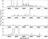 |
Fig. A.1. The full MUSE spectrum of RU Lupi extracted at the source position with an aperture of radius 98 au. |
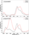 |
Fig. A.2. The MUSE [O I] λ6300 and [S II] λ6731 emission line profiles. The red profiles display the spectra extracted using a circular aperture of radius 14 au from the source position. The black profiles display the spectra extracted using a circular aperture of radius 14 au from the jet knot position located at approximately 85 au along the jet. |
Appendix B: Line to continuum ratio maps
Line to continuum ratio plots are an effective tool for investigating the contribution of scattered emission to intrinsic line emission (Delabrosse et al. 2024; Birney et al. 2024). These figures display the result of calculating the ratio between an integrated line image, before continuum subtraction, and an integrated continuum image that is taken spectrally nearby to the line of interest. An assumption is made that the scattered emission is entirely light from the driving source of the outflow scattered off the disk and surrounding nebulous material. Therefore, the contribution from scattered light to the integrated line images will be represented by a constant ratio in these plots, as the scattered light follows the same spatial distribution as the continuum emission. In contrast, the real, intrinsic local emission will appear bright in these images, exceeding the constant ratio that represents the contribution from scattered light.
Figure B.1 displays the line to continuum ratio plots for the [O I] λ6300, [S II] λ6731 and [N II] λ6583 channel maps shown in Figs. 2, before continuum subtraction and deconvolution (see Sect. C for the channel maps before and after deconvolution). A sector of the ALMA 1.3 mm dust continuum disk image is shown in white contours (Andrews et al. 2018). In the high-velocity channels (HVC2) one sees the intrinsic collimated jet emission extending from the source position and culminating in a jet knot at an offset from the source of approximately 85 au. In the intermediate velocity channel (HVC1) one also sees the base of the outflow in intrinsic line emission, but comparatively less collimated than the jet emission seen in the HVC2 line to continuum ratio maps.
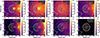 |
Fig. B.1. Line to continuum ratio maps of the [O I] λ6300, [S II] λ6731 and [N II] λ6583 channel maps shown in Figs. C.1 and C.2, before continuum subtraction and deconvolution. A sector of the ALMA 1.3 mm dust continuum disk image is shown in white contours. Intrinsic line emission appears bright in these images, whereas scattered light is represented by a constant ratio close to unity. The red arrow delineates the disk PA and radius from Huang et al. (2018) (121° ± 5°, 63 ± 1 au) and the green dashed line represents the jet PA measured here (213° ± 2°). |
Also present in the jet and HVC1 line to continuum ratio maps is a wide, arc-like feature, located just beyond the jet knot at 85 au seen in the HVC2 channels. This arc-like feature is not detected in the channel maps shown in Figs. C.1 and C.2. Intrinsic emission in line to continuum ratio maps appears brighter as offset from the source increases as the contribution from scattered light decreases with distance from the source. As this wide arc-like feature is not detected in the channel maps, it is likely that it is intrinsic, very low-intensity line emission that appears bright in the line to continuum maps, as the contribution from scattered light is very low in the region, resulting in a large line to continuum ratio. As the feature displays an arc-like morphology, it may indicate the location of the edge of the gas disk surrounding RU Lupi, where the inner edge of the arc-like feature is the outer edge of the gas disk. Small dust particles responsible for scattering at optical wavelengths follow the spatial distribution of the gas disk, that can extend two to three times further than mm dust disk. As the contribution from scattered light is likely very low in the region where the the arc-like feature is located, this indicates a rapid decrease in the density of scattering particles which would coincide with the gas disk edge.
In the low-velocity channels (LVC) one sees intrinsic wide-angled outflow emission, that is comparatively dimmer than the jet emission. In the high-velocity redshifted [S II] λ6731 emission, labelled Redshifted in Fig. B.1 one sees an intrinsic knot of line emission at an offset of approximately 100 au from the source position, in the opposite direction of the blueshifted outflow. In the HVC1 and LVC channels in [O I] λ6300 emission, one sees significant line emission across the FOV. We attribute this emission to residual scattered line emission from the outflow, that does not follow the same spatial distribution as scattered light from the source, resulting in the outflow emission illuminating surrounding ambient material.
Appendix C: Results before and after deconvolution
Figures C.1 and C.2 display the channel maps before (top panels) and after (bottom panels) the Lucy-Richardson deconvolution is applied. An assumption was made when estimating the PSF used for the deconvolution, in that the local continuum emission was used as the PSF. The PSFs used when deconvolving the [O I] λ6300, [S II] λ6731, and [N II] λ6583 emission are shown in Fig. C.3. The deconvolution was allowed to run for 20 iterations to enhance the morphology of the outflow without introducing any artefacting. The jet knot at ∼ 85 au is marginally visible before deconvolution in the high-velocity channels. The possible high-velocity [S II] λ6731 redshifted knot is also visible before deconvolution.
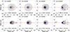 |
Fig. C.1. Comparing the channel maps of the jet, HVC1 and NC in [O I] λ6300 emission, and the jet in [N II] λ6583 emission, before (top panels) and after (bottom panels) deconvolution. The source position is marked with a blue star. The contour levels begin at 3σ of the background emission and increase by factors of 1.5. |
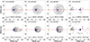 |
Fig. C.2. Comparing the channel maps of the jet, HVC1 and NC in [S II] λ6731 emission, and the high-velocity redshifted knot, also in [S II] λ6731 emission, before (top panels) and after (bottom panels) deconvolution. The source position is marked with a blue star. The contour levels begin at 3σ of the background emission and increase by factors of 1.5. |
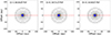 |
Fig. C.3. The PSFs used when deconvolving the [O I] λ6300, [S II] λ6731, and [N II] λ6583 emission. The source position is marked with a blue star. The contour levels begin at 3σ of the background emission and increase by factors of 1.5. |
Appendix D: Transverse PV diagrams and line profiles
Figure D.1 presents position velocity (PV) diagrams, in [O I] λ6300 and [S II] λ6731 emission, transverse to the outflow axis extracted at different distances along the outflow, namely, 0 au, 10 au, 50 au, and 80 au (0 au, 29 au, 145 au, and 232 au deprojected) from the source position. Initially, two velocity components are present; the jet, which is seen at all distances, and the NC, which fades as distance from the driving source of the outflow increases. This evidences that the NC is a separate outflow component to the jet. In order to better illustrate the presence of two distinct velocity components in the position velocity diagrams made transverse to the outflow axis, line profiles are extracted along the 0 au offset position, indicated by a horizontal red dashed line in Fig. D.1. In accordance with Fig. D.1, these line profiles are extracted from the [O I] λ6300 and [S II] λ6731 emission line regions at distances of 0 au, 10 au, 50 au, and 80 au from the source position, and are presented in Fig. D.2. There are two distinct velocity components in the line profile, the jet and the NC. The NC is seen to decrease in intensity as the distance from the source increases. In contrast, the jet emission remains strong as the distance increases. The NC is not detected at the source position in the [S II] λ6731 line which is likely an effect of the lines critical density. One only begins to see the NC in [S II] λ6731 as the density decreases further from the driving source. Whelan et al. (2021) report no [S II] λ6731 emission in the NC within 2 au (8 au deprojected) of the source.
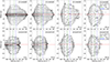 |
Fig. D.1. Position Velocity diagrams made transverse to the outflow axis for the [O I] λ6300 and [S II] λ6731 emission line regions. Slices were extracted at the source position and at distances of 10 au, 50 au and 80 au from the star. Distances are not deprojected and these positions correspond to 29 au, 145 au and 232 au when corrected for the inclination of the system. The velocities of the jet, HVC1 and NC as measured by Whelan et al. (2021) are marked by the dashed lines. The NC appears as a clear second component distinct from the jet. The contour levels begin at 3σ of the background emission and increase by factors of 1.5. |
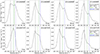 |
Fig. D.2. Line profiles extracted along the 0 au offset position (red dashed line) from the position velocity diagrams made transverse to the outflow axis, shown in Fig. D.1, for the [O I] λ6300 and [S II] λ6731 emission line regions. These PV slices were extracted at the source position, and at distances of 10 au, 50 au and 80 au from the star. Distances are not deprojected and these positions correspond to 29 au, 145 au and 232 au when corrected for the inclination of the system. The velocities of the jet, HVC1 and NC as measured by Whelan et al. (2021) are marked by the dashed lines. The line flux decreases as the offset from the central source increases. The NC appears as a clear secondary component distinct from the jet. |
Appendix E: Aperture size for spectral extraction
Figure E.1 displays how the measured flux and mass accretion rate (Ṁacc) increase as the radius of the spectral extraction aperture placed at the source position increases. This analysis was performed using the Hβλ4861 and O I λ7773 emission lines to provide confirmation that this effect is present throughout the spectral axis. The angular resolution of the observation after adaptive optics is ∼ 0 07, and the seeing is 0
 45. However, utilising the observations seeing as the aperture size, an aperture radius of ∼ 0
 23, for spectral extraction would result in a significant portion of the line flux not being accounted for, existing outside of the aperture radius. We instead chose to select an aperture size where both the line flux and consequently, the resulting mass accretion rate, begin to asymptote to a constant value. We choose an aperture radius of 0
 7 (98 au) to extract spectra from the source position. This is approximately three times the seeing of the observation. The results shown in Fig. E.1 points to a large aperture for correction factor for MUSE NFM data, as could be expected due to MUSE’s extended PSF wings. However, it is likely that the scattering discussed above is contributing to the flux at all wavelengths and that emission from the base of the outflow and accretion shocks would also be scattered, as well as contribution to emission from the disk surface, artificially inflating the measured line luminosities.
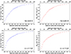 |
Fig. E.1. Hβλ4861 and O I λ7773 flux (left panels) and Ṁacc (right panels) as a function of aperture radius size. The aperture size in units of au is also displayed, calculated using the distance to RU Lupi (d ∼ 140 pc). |
Appendix F: Mass accretion rate results
The accretion tracing emission lines are presented in Table F.1. The mass accretion rates are derived following the method of Alcalá et al. (2017). The Hα and [Ca II] lines were not used due to saturation at the source position. The mass accretion rate derived from the [O I] λ6300 line was not used in the mean calculation, as we use this line to measure the mass outflow rates in the jet and NC. Notice the large uncertainties on Ṁacc that are common when using line luminosities to estimate the mass accretion rate (See Sect. 4). The estimated extinction for RU Lupi is ∼ 0 (Fang et al. 2018).
Accretion luminosities and mass accretion rates in the different line tracers. Hα and the [Ca II] triplet are saturated at the source position and thus could not be used as reliable accretion tracers. Furthermore, the mass accretion rate derived from the [O I] λ6300 line was not used in the mean calculation, as we use this line to measure the mass outflow rates in the jet and NC.
Appendix G: Outflow centroid positions
Outflow centroid measurements of the jet, HVC1 and NC in [O I] λ6300, [S II] λ6731 and [N II] λ6583 emission measured along the outflow with the driving source position at the origin are presented in Fig. G.1. These outflow centroid are measured in the velocity component channel maps before deconvolution. The error bars on the data points are the difference in centroid position as measured in the pre-deconvolved channel maps and deconvolved channel maps. Centroid measurements as measured from the spectro-astrometry presented in Whelan et al. (2021) are over-plotted in magenta. The centroid measurements do not reveal any significant deviations from the position of the outflow axis, neither do they display any prominent outflow wiggling.
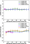 |
Fig. G.1. Outflow centroid measurements of the jet, HVC1 and NC in [O I] λ6300, [S II] λ6731 and [N II] λ6583 emission measured along the outflow with the driving source position at the origin. Centroid measurements as measured from the spectro-astrometry presented in Whelan et al. (2021) are over-plotted in magenta. |
Appendix H: 0104.C-0919(B) Observations
RU Lupi was also observed by MUSE in NFM in Summer 2021 as part of the programme 0104.C-0919 (B). These data were also analysed, and in Figs. H.1 and H.2, we display the channel maps in [O I] λ6300, [S II] λ6731 and [N II] λ6583 emission before (top panels) and after (bottom panels) deconvolution prepared from this data. Although the morphological features identified in the channel maps are present here, comparing with Figs. C.1 and C.2 shows the data to have a lower S/N. Additionally, these data were affected by a MUSE artefact known as a spike (MUSE manual: Section 3.9.1)5. This affected the [O I] λ6300 channel maps significantly causing the measured PA to be different than the other outflow tracing lines, and for the emission to appear asymmetric. We therefore chose to make use of the 106.21EN.001 observations in our analysis.
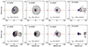 |
Fig. H.1. Comparing the channel maps produced using the 0104.C-0919(B) data of the jet, HVC1 and NC in [O I] λ6300 emission, and the jet in [N II] λ6583 emission, before (top panels) and after (bottom panels) deconvolution. The contour levels begin at 3σ of the background emission and increase by factors of 1.2. |
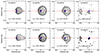 |
Fig. H.2. Comparing the channel maps produced using the 0104.C-0919(B) data of the jet, HVC1 and NC in [S II] λ6731 emission, and the high velocity redshifted knot, also in [S II] λ6731 emission, before (top panels) and after (bottom panels) deconvolution. The contour levels begin at 3σ of the background emission and increase by factors of 1.2. |
All Tables
Accretion luminosities and mass accretion rates in the different line tracers. Hα and the [Ca II] triplet are saturated at the source position and thus could not be used as reliable accretion tracers. Furthermore, the mass accretion rate derived from the [O I] λ6300 line was not used in the mean calculation, as we use this line to measure the mass outflow rates in the jet and NC.
All Figures
|
Fig. 1. Integrated (vrad = 270 − 325 km s−1) [S II] λ6731 continuum-subtracted image of the RU Lupi jet with a sector of the ALMA 1.3 mm dust continuum disk image shown in white contours (Andrews et al. 2018). The ALMA beam size (3.5 × 3.4 au) is shown in the lower left corner. The red arrow delineates the disk PA and radius from Huang et al. (2018) (121° ± 5°, 63 ± 1 au), and the dashed green line shows the jet PA measured here (213° ± 2°). The jet and outer knot are perpendicular to the disk, but the inner bright region of the jet at < 50 au from the source is asymmetric about the green line. |
| In the text | |
|
Fig. 2. Deconvolved channel maps of the jet, HVC1, and NC emission from RU Lupi in the [O I] λ6300, [S II] λ6731 and [N II] λ6583 emission lines. The distances are not deprojected, and the red box shows the region for which the outflow widths are mapped (Fig. 3). The source position is marked with a blue star. The contour levels begin at 3σ of the background emission and increase by factors of 1.5. |
| In the text | |
|
Fig. 3. Full width at half maximum (left panels) and normalised flux (right panels) measurements of the jet, HVC1, and NC in [O I] λ6300, [S II] λ6731 and [N II] λ6583 emission, measured along the outflow, with the driving source position at the origin. The error bars on the FWHM data points are the uncertainty of the FWHM in the Gaussian fitting routine, which appear small here due to the high S/N of the transverse spatial profiles. In the right panels, the jet emission follows a different pattern than the HVC1 and NC, indicating an unresolved knot in the jet. The wind height is measured as the width of the NC emission at half the peak flux. |
| In the text | |
|
Fig. A.1. The full MUSE spectrum of RU Lupi extracted at the source position with an aperture of radius 98 au. |
| In the text | |
|
Fig. A.2. The MUSE [O I] λ6300 and [S II] λ6731 emission line profiles. The red profiles display the spectra extracted using a circular aperture of radius 14 au from the source position. The black profiles display the spectra extracted using a circular aperture of radius 14 au from the jet knot position located at approximately 85 au along the jet. |
| In the text | |
|
Fig. B.1. Line to continuum ratio maps of the [O I] λ6300, [S II] λ6731 and [N II] λ6583 channel maps shown in Figs. C.1 and C.2, before continuum subtraction and deconvolution. A sector of the ALMA 1.3 mm dust continuum disk image is shown in white contours. Intrinsic line emission appears bright in these images, whereas scattered light is represented by a constant ratio close to unity. The red arrow delineates the disk PA and radius from Huang et al. (2018) (121° ± 5°, 63 ± 1 au) and the green dashed line represents the jet PA measured here (213° ± 2°). |
| In the text | |
|
Fig. C.1. Comparing the channel maps of the jet, HVC1 and NC in [O I] λ6300 emission, and the jet in [N II] λ6583 emission, before (top panels) and after (bottom panels) deconvolution. The source position is marked with a blue star. The contour levels begin at 3σ of the background emission and increase by factors of 1.5. |
| In the text | |
|
Fig. C.2. Comparing the channel maps of the jet, HVC1 and NC in [S II] λ6731 emission, and the high-velocity redshifted knot, also in [S II] λ6731 emission, before (top panels) and after (bottom panels) deconvolution. The source position is marked with a blue star. The contour levels begin at 3σ of the background emission and increase by factors of 1.5. |
| In the text | |
|
Fig. C.3. The PSFs used when deconvolving the [O I] λ6300, [S II] λ6731, and [N II] λ6583 emission. The source position is marked with a blue star. The contour levels begin at 3σ of the background emission and increase by factors of 1.5. |
| In the text | |
|
Fig. D.1. Position Velocity diagrams made transverse to the outflow axis for the [O I] λ6300 and [S II] λ6731 emission line regions. Slices were extracted at the source position and at distances of 10 au, 50 au and 80 au from the star. Distances are not deprojected and these positions correspond to 29 au, 145 au and 232 au when corrected for the inclination of the system. The velocities of the jet, HVC1 and NC as measured by Whelan et al. (2021) are marked by the dashed lines. The NC appears as a clear second component distinct from the jet. The contour levels begin at 3σ of the background emission and increase by factors of 1.5. |
| In the text | |
|
Fig. D.2. Line profiles extracted along the 0 au offset position (red dashed line) from the position velocity diagrams made transverse to the outflow axis, shown in Fig. D.1, for the [O I] λ6300 and [S II] λ6731 emission line regions. These PV slices were extracted at the source position, and at distances of 10 au, 50 au and 80 au from the star. Distances are not deprojected and these positions correspond to 29 au, 145 au and 232 au when corrected for the inclination of the system. The velocities of the jet, HVC1 and NC as measured by Whelan et al. (2021) are marked by the dashed lines. The line flux decreases as the offset from the central source increases. The NC appears as a clear secondary component distinct from the jet. |
| In the text | |
|
Fig. E.1. Hβλ4861 and O I λ7773 flux (left panels) and Ṁacc (right panels) as a function of aperture radius size. The aperture size in units of au is also displayed, calculated using the distance to RU Lupi (d ∼ 140 pc). |
| In the text | |
|
Fig. G.1. Outflow centroid measurements of the jet, HVC1 and NC in [O I] λ6300, [S II] λ6731 and [N II] λ6583 emission measured along the outflow with the driving source position at the origin. Centroid measurements as measured from the spectro-astrometry presented in Whelan et al. (2021) are over-plotted in magenta. |
| In the text | |
|
Fig. H.1. Comparing the channel maps produced using the 0104.C-0919(B) data of the jet, HVC1 and NC in [O I] λ6300 emission, and the jet in [N II] λ6583 emission, before (top panels) and after (bottom panels) deconvolution. The contour levels begin at 3σ of the background emission and increase by factors of 1.2. |
| In the text | |
|
Fig. H.2. Comparing the channel maps produced using the 0104.C-0919(B) data of the jet, HVC1 and NC in [S II] λ6731 emission, and the high velocity redshifted knot, also in [S II] λ6731 emission, before (top panels) and after (bottom panels) deconvolution. The contour levels begin at 3σ of the background emission and increase by factors of 1.2. |
| In the text | |
Current usage metrics show cumulative count of Article Views (full-text article views including HTML views, PDF and ePub downloads, according to the available data) and Abstracts Views on Vision4Press platform.
Data correspond to usage on the plateform after 2015. The current usage metrics is available 48-96 hours after online publication and is updated daily on week days.
Initial download of the metrics may take a while.