| Issue |
A&A
Volume 692, December 2024
|
|
|---|---|---|
| Article Number | A54 | |
| Number of page(s) | 25 | |
| Section | Catalogs and data | |
| DOI | https://doi.org/10.1051/0004-6361/202451744 | |
| Published online | 02 December 2024 | |
H I line observations of 290 evolved stars made with the Nançay Radio Telescope
I. Data
1
GEPI, Observatoire de Paris, Université PSL,
5 place Jules Janssen,
92190
Meudon,
France
2
Observatoire Radioastronomique de Nançay, Observatoire de Paris, Université PSL, Université d’Orléans,
18330
Nançay,
France
3
Massachusetts Institute of Technology Haystack Observatory,
99 Millstone Road,
Westford,
MA
01886,
USA
4
LERMA, Observatoire de Paris, Université PSL,
61 av. de l’Observatoire,
75014
Paris,
France
★ Corresponding author; This email address is being protected from spambots. You need JavaScript enabled to view it.
Received:
31
July
2024
Accepted:
15
October
2024
Abstract
We present a compendium of H I 21-cm line observations of circumstellar envelopes (CSEs) of 290 evolved stars, mostly (~84%) on the asymptotic giant branch (AGB), made with the 100 m-class, single-dish Nançay Radio Telescope. The observational and data reduction procedures were optimised to separate genuine CSE H I emission from surrounding Galactic line features. For most targets (254), the results have not been previously published. Clear detections were made of 34 objects, for 33 of which the total H I flux and the size of the CSE could be determined. Possible detections were made of 21 objects, and upper limits could be determined for 95 undetected targets, while for 140 objects confusion from Galactic H I emission along the line of sight precluded meaningful upper limits. The collective results of this survey can provide guidance on the detectability of circumstellar H I gas for future mapping and imaging studies.
Key words: stars: AGB and post-AGB / circumstellar matter / stars: winds, outflows / radio lines: stars
Deceased.
© The Authors 2024
 Open Access article, published by EDP Sciences, under the terms of the Creative Commons Attribution License (https://creativecommons.org/licenses/by/4.0), which permits unrestricted use, distribution, and reproduction in any medium, provided the original work is properly cited.
This article is published in open access under the Subscribe to Open model. This email address is being protected from spambots. You need JavaScript enabled to view it. to support open access publication.
1 Introduction
Observations in the 21-cm H I line provide a powerful tool for the study of various properties of the circumstellar envelopes (CSEs) of mass-losing asymptotic giant branch (AGB) stars and other types of evolved stars, which cannot be determined through other spectral lines. For example, such observations can trace gas beyond the CO dissociation radius, probe the interface between the star and the interstellar medium (ISM), and provide independent estimates of the total masses and ages of CSEs.
Once stars leave the main sequence and reach the giant branch, they start losing mass (in the form of gas and dust) through stellar winds; see, e.g. Marengo (2015), Höfner & Olofsson (2018), Decin (2021), and Matthews (2024). On the AGB, mass-loss rates range from several 10−8 M⊙ yr−1 up to 10−4 M⊙ yr−1, with the bulk of the mass loss occuring in the form of hydrogen. The stars become surrounded by CSEs, whose gaseous constituents can be studied using atomic and molecular spectral lines. The winds are accelerated through the coupling between grains and gas, from the stellar atmosphere (at a few stellar radii) up to the outer CSE (at radii of thousands of AU) where the wind starts to interact with the interstellar medium (ISM), often forming bow shocks in the case where the star is moving supersonically relative to the ambient medium.
Under the influence of the interstellar ultraviolet (UV) radiation field, the chemical constituents of the CSE are progressively dissociated. One of the best studied ones is the CO molecule, which has strong rotational lines at a low excitation temperature. However, as it is photodissociated at small radii (see, e.g. Saberi et al. 2019), it is difficult to accurately derive a total mass for all constituents in the CSE based only on CO line measurements.
Thus, H2 (through the CO lines) and H I are essential constituents to track throughout the CSE (see, e.g. Glassgold & Huggins 1983). While H2 has no dipole moment and is difficult to observe through its vibrational transitions corresponding to high excitation temperatures, H I may be either nascent in a hot atmosphere (T > 2500 K) or produced by the photodissociation of H2 at large radii.
This paper presents an overview of the results of H I 21-cm line observations of evolved stars made with the 4′ × 22′ beam of the 100m-class single-dish Nançay Radio Telescope (NRT). The results represent an investment of ~5000 hours of telescope time since 1992. A total of 290 stars were observed, and for most (254, or 88%), the results have not been previously reported. These include upper limits for non-detections, as well as identification of cases for which any circumstellar H I line emission was completely confused with Galactic H I clouds along the line of sight and where no conclusion can be drawn about the presence of H I in the CSE. This information is nonetheless useful for guiding selection of targets for future surveys of circumstellar H I at a higher angular resolution. Results of NRT H I observations of 36 stars from our sample have been previously published in Le Bertre & Gérard (2001, 2004), Gérard & Le Bertre (2003, 2006), Gardan et al. (2006), Libert et al. (2007, 2008, 2010a,b), Matthews et al. (2008), Gérard et al. (2011), and Le Bertre et al. (2012).
Follow-up H I imaging and mapping observations carried out with the Very Large Array (VLA) and the Green Bank Telescope of 16 AGB stars and red supergiants initially observed with the NRT were reported in Matthews & Reid (2007); Matthews et al. (2008, 2013, 2015) Le Bertre et al. (2012), and Hoai et al. (2014) (see also Table B.2, and online Tables 5 and 6). In VLA imaging studies with a resolution of ~1′, H I was detected in 13 cases. The morphologies of the H I distributions are quite varied, showing detached shells around the star (IRC +10216, Y CVn, V1942 Sgr, Y UMa, and α Ori), blobs of H I offset from the AGB (EP Aqr and R Cas), head-tail structures (o Cet, RS Cnc, X Her, and TX Psc), a shell-tail structure (RX Lep), and one object (R Peg) with a peculiar ‘horseshoe’-shaped H I morphology. The three stars that were not detected in H I with the VLA are RAFGL 3099, R Aqr, and IK Tau. Furthermore, no H I was detected in W Hya at the VLA by Hawkins & Proctor (1993).
A challenge for observing circumstellar H I is that the detection can be severely hindered, if not made downright impossible, owing to the presence of ubiquitous Galactic H I emission along the line of sight. This applies in particular to observations made with single-dish radio telescopes that rely on emission-free off- source reference position spectra (see, e.g. Matthews et al. 2013 for further details). Confusion by ubiquitous, and often strong, Galactic H I signals has been a major issue with the NRT data throughout the project (see Sections 3 and 5). Although the relatively good 4′ spatial resolution of the NRT in right ascension was a favourable factor in dealing with this confusion, in declination the beam size is much larger, ≥22′.
The present catalogue includes a new assessment of all NRT spectra in terms of confusion by Galactic H I, including for previously published NRT results. This is based on new experience gained, including the analysis of additional NRT H I observations that were made of many sources with a wider range of east-west off-source positions as well as of positions 11′ (0.5 north-south HPBW) north and south of the star, and the use of more recently published radial velocities. Our ultimate aim is to contribute to the understanding of the fate of the major constituent ejected by evolved stars during their evolution, that is, hydrogen.
In the present paper, we want to provide guidance for other studies of evolved stars in terms of detectability of H I in CSEs based on our single-dish telescope observations, in particular for follow-up imaging and mapping studies carried out at a (much) higher spatial resolution with interferometers or single-dish telescopes with smaller beam sizes. For a number of undetected stars, we obtained sensitive upper limits (in some cases based on up to 100 hours of integration) that provide robust constraints on the probability of detection with other telescopes.
Unless otherwise indicated, all radial velocities are in the local standard of rest (LSR) reference frame. They were calculated based on the conversion from heliocentric to LSR velocities given in Kerschbaum & Olofsson (1999) (see Section 4 for details).
This paper is organised as follows. In Section 2 the selection of the observed AGB stars is described and Section 3 discusses the observations and data reduction. Results are presented in Section 4 and further discussed in Section 5. Conclusions are summarised in Section 6. Comments on the determination of H I profiles are given in Appendix A for selected sources.
2 Sample selection
Our targets were primarily chosen from lists of well-studied, nearby objects classified as evolved stars and related objects. Our final sample of 290 evolved stars mostly consists of AGB stars (for ~84%), but other types were observed as well, to broaden the scope of our studies of CSEs in H I. We did not apply strict criteria for the selection of stars to be observed; these changed as the project developed over the past three decades.
The names of the 27 stars which are clearly not AGB are flagged with an ‘n’ in the Tables. They include eight planetary nebulae, six high proper motion stars, five post-AGB stars, and four red supergiants. The 19 cases for which we consider their classification as AGB dubious are flagged with a ‘d’.
The stars’ variability types we used are primarily based on the General Catalogue of Variable Stars, GCVS (Samus’ et al. 2017); see Section 4 for further details. In terms of their variability classification, the main categories are: mira (119 = 41%), SRb (70 = 24%), Lb (28 = 10%), SRc (12 = 4%), and SRa (7 = 2%).
We did not select on mass-loss rates, as derived from CO line observations. The observed stars span a wide range of massloss rates, of three orders of magnitude, from 2 × 10⁻⁸ to 2 × 10⁻⁵ M⊙ yr−1.
All targets were selected without avoiding either low Galactic latitudes or small radial LSR velocities, where confusion by Galactic H I clouds is the most likely: 57 targets (20%) have |b| < 10°, and 73 (25%) have |VLSR| < 10 km s−1. Many are located at right ascensions outside the Galactic Centre range, where the overall time pressure on the meridian-type NRT is lower and where (very) long integrations, of up to 100 hours per source, could therefore be made. The radial velocities of most (76%) of our targets were measured in radio spectral lines (CO, OH, H2O, SiO), the others in optical lines.
3 Observations and data reduction
The 100m-class Nançay Radio Telescope is a Kraus/Ohio State meridian transit-type instrument. It consists of a fixed spherical mirror (300 m long and 35 m high), a tiltable flat mirror (200 × 40 m), and a focal carriage moving along a curved rail track. Its collecting area is about 7000 m2 . Due to its elongated geometry some of the instrument’s characteristics, such as gain and north-south beam size, depend on the observed declination. It can observe down to a declination of −39°. At 21 cm wavelength its half-power beam width (HPBW) is always 4′ in right ascension, whereas in declination it increases from 22′ at δ<20° to 34′ at δ = 75°. Sources on the celestial equator can be tracked for about 60 minutes.
Our first observations were made in 1992 and 1993 of 103 sources, 67 of which were reobserved a decade later, after a major renovation of the telescope, and the last observations were made in 2017. More than 5000 hours of telescope time were used in total for the project. Total integration times per source varied considerably, from one hour to 100+ hours. Telescope time allocation permitting, we spent more time on sources that were faint (as was often the case with miras) and/or whose large angular sizes required observations with multiple off-source pointing positions (see Sect. 3.2).
In 1992 and 1993 data were acquired using a 1024-channel autocorrelator, with half the frequency channels used for observations in the left- or right-handed circular polarisation, respectively. The total bandwidth was 0.4 MHz, or 84.4 km s−1, at the rest frequency of 1420.40 MHz. After boxcar smoothing in velocity and averaging of both polarisations, the final spectrum consisted of 128 channels with a velocity resolution of 0.66 km s−1. The system temperature was 37 K at zero declination. The observing procedure consisted of position switching using only two off-source positions, located one HPBW east and one HPBW west of the star.
In the late 1990s the NRT underwent a major renovation, including the installation of corrugated horns in an optimised dual-reflector offset Gregorian mirror system, which increased its sensitivity by a factor of 2.2; see van Driel et al. (1997) and Granet et al. 1999). Starting in 2001, observations were made with a new 8192 channel autocorrelator, split into 4 banks of 2048 channels each for simultaneous observations in two orthogonal linear polarisations (PA = 0o and 90o), and in left- and right-hand circular polarisations. The H I emission is thermal and unpolarised. For the observations presented here the Stokes total intensity parameter I was formed by adding the two circular polarisations. In order to identify possible receiver instabilities or radio frequency interference (RFI), we also formed the Stokes I by adding the two orthogonal linear polarisations. In practice, our observations were not affected by RFI. The terrain surrounding the NRT site acts as a natural barrier against unwanted terrestrial radio emissions.
The velocity coverage was 165 km s−1 and the maximum velocity resolution 0.08 km s−1. However, almost all spectra presented here were later smoothed to a resolution of 0.32 km s−1. The typical system temperature was 30 K near the celestial equator. Linear baselines were fitted to the averaged spectra, and subtracted.
Our searches for circumstellar H I emission were centred on the most accurate published systemic velocity of the target available at the time. In some cases the velocity we used for our current analysis is slightly different owing to the availability of updated information (see Section 4 for details). However, in no cases has this significantly impacted the interpretation of the data.
For observations made from 2001 onwards in position switching mode we used more east-west off-source positions than we did in 1992 and 1993, and we also observed positions to the north and south of the star, to investigate, respectively, east-west and north-south source sizes. Our standard procedure consisted of alternating between an on-source position and two off-source positions, located symmetrically towards the east and west of the on-source position (see Section 3.1 for further details). In all position-switching observations the same amount of integration time was used pointing towards each of the three positions observed: on-source, off-source east, and off-source west.
Most sources were also observed in frequency-switching mode while pointing at the stellar position. This allows the accurate measurement of the background brightness temperature in the expected H I velocity range of the CSE, and to estimate the confusion level due to the telescope’s sidelobes (see Section 3.1).
The effective bandwidth was 1.53 MHz (323 km s−1), centred on the stellar velocity. The receiver bandwidth was set to 1.56 MHz (329 km s−1) and a frequency switch of +1.53 MHz (−323 km s−1) was used, as this corresponds to exactly three times the 0.51 MHz frequency of the ripple in the spectral baseline that is often caused by specular reflection between telescope structures (see, e.g. Wilson et al. 2009). Choosing this offset thus cancels out the baseline ripple. Furthermore, the negative offset in velocity avoids contamination by possible extragalactic H I emission.
NRT flux scale calibration is based on long-term, regular monitoring of radio sources by NRT staff. It consists of observations of 20 continuum calibration sources every 3 months, monthly observations of the primary calibrator 3C 123 and weekly observations of the continuum source 3C 161 and the line source W12. Calibrator flux densities are based on Baars et al. (1977). The scatter in the measurements on which the absolute flux density scale is based is ~5% at 1410 MHz. All data were reduced using the standard NRT software packages NAPS and SIR, developed by NRT staff and telescope users.
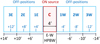 |
Fig. 1 Diagram illustrating examples of on- and off-source NRT beam positions that were used to estimate the east-west diameters, and peak- and total H I profiles of the observed sources (see Sect. 3.2). The eastwest HPBW is 4', but we note that in reality the NRT beam is relatively more elongated in the north-south direction (≥22′) than is shown here. |
3.1 Dealing with Galactic H I confusion
Detecting genuine CSE H I emission among the ubiquitous Galactic clouds can be a major challenge in terms of both observing procedure and data analysis. This applies in particular for sources near the Galactic plane, and for single-dish radio telescopes like the NRT whose north-south beam size is relatively large (≥22′). The H I peak flux densities we measured within the central NRT beam for clear detections range between 0.9 and 0.007 Jy. Since the brightness of the Galactic H I emission typically spans a range between 1 and 100 Jy, the maximum source-to-background contrast ratio is expected to vary from about 0.5 to 0.005 in practice – the smaller values occur close to the Galactic plane.
We note that the H I spectra presented here use data from only a single on-source position for each target, centred on the coordinates of the star. Previous studies have shown our use of off-source positions symmetrically to the east and to the west of the star to be an effective scheme for separating CSE emission from Galactic line signals in NRT spectra (e.g. Gérard & Le Bertre 2006).
This procedure works best when the intensity of the Galactic background has a linear variation with position in the region surrounding the target source. However, if its variation is quadratic, or of even higher order, spurious spectral features may appear. However, as these generally grow rapidly with increasing separation between the two off-source positions, this allows us to identify them.
The principles of our east-west on-off source position scheme are illustrated in Fig. 1. We will refer to the angular separation between the on-source and an off-source position as a “throw amplitude”, and use the notation CnEW to indicate spectra obtained using a throw amplitude of n HPBWs to the east and west of the target position (denoted as C in the Figure).
We have used east-west throw amplitudes ranging from 1'3 to 48' (i.e. from 0.3 to 12 HPBWs), in order to cover a large range of potential CSE sizes. Examples of spectra obtained with a broad range of east-west throw amplitudes are shown in Fig. 2 for selected sources that were classified as either clear detections, upper limits, or confused.
The impact on the detectability of CSEs in H I caused by increasing levels of confusion due to Galactic lines is illustrated in the examples shown in Fig. 1:
When the Galactic H I emission is weak, the signal from a genuine CSE detection increases with throw amplitude and converges once both off-source positions lie outside the CSE: V1942 Sgr is a good example.
On the other hand, when the Galactic emission dominates the H I signal continues to increase with the throw amplitude: W Cas, HV Cas and AQ And are good examples. The stronger the Galactic confusion, the earlier the profiles start diverging when the throw amplitude is increased. We therefore often observed with a very small throw amplitude of 1.′3 (C0.33EW), which reduces the confusing H I signal more than it does the genuine CSE line emission.
In intermediate cases (e.g. TX Psc), genuine CSE H I emission is seen at the CO line velocity (12 km s−1), which peaks for a throw amplitude of 6′ , while a Galactic emission feature grows rapidly near 10 km s−1 and dominates at a throw amplitude of 12′ .
The intermediate case examples also illustrate the advantage of the high velocity resolution used (typically 0.32 km s−1) in distinguishing between CSE emission and a confusing, Galactic feature along the line of sight that occurs close to the stellar velocity.
In the north-south direction the NRT HPBW is ≥22′ , considerably larger than the 4′ along the east-west axis. For the two reasons mentioned hereafter, we also obtained observations towards positions 11′ to the north and to the south of the star. The off-positions used for these north-south pointings are in general located one east-west HPBW (4′) to the east and to the west of them, but for some large sources additional off-positions with east-west throws of up to 24′ were used.
These observations were made of all clear detections, as well as of many other sources. However they were not made for the weakest, as this would have required a prohibitive amount of additional telescope time.
The two reasons for which the north-south observations were made are to check if the source is extended in the north-south direction, or if the detection is confused by ISM emission along the line of sight:
-
If a source is north-south extended, using only east-west pointings at the declination of the star (as we did for the fluxes given in this paper) would underestimate its measured flux.
For an unresolved source, at both pointings 11′ (0.5 north-south HPBW) north and south of the star we would expect to measure half of the integrated line flux that was observed when pointing towards the star. Using this criterion, very few cases showed indications of being resolved in the north-south direction. However, a difference between the north and south position fluxes could also in principle be due to confusing ISM emission (see below).
An indication of the expected north-south sizes could in principle be deduced from the east-west NRT source sizes estimated for the 33 clear detections, under the assumption that the sizes in both directions are similar (to be examined using VLA images). We note that (1.) Only four of the 33 sources (12%) have estimated NRT east-west diameters significantly larger than the 22′ NRT north-south HPBW, whereas nine (27%) have diameters of 20′ , that is, similar to the HPBW. (2.) Among the 12 published VLA H I maps of sources in our sample only three show similar east-west and north-south sizes, whereas others have quite varied morphologies which often makes such a comparison impossible. Furthermore, none of the 12 would have been resolved by the NRT north-south HPBW (see Sections 1 and 5).
The larger north-south beam size introduces a possible risk of confusion with ISM emission along the line of sight, but it is difficult to ascertain from NRT data where exactly these confusing sources are located once their presence is suspected. Comments on confusion deduced from NRT observations can be found in Appendix A for IRC +10216, S CMi, U CMI, TX Psc, and AQ Sgr. In practice, the much smaller beam size of the VLA is required to locate confusing sources, as was done in the case of X Her (see Sect. 5).
We note that the spectra obtained pointing towards the star and towards positions to the north and south of the star have not been combined for the analysis of the NRT results (see Sect. 3.2). This was because they were made for different purposes; for example, the former to estimate east-west source sizes, and the latter to check if sources are north-south resolved.
We assume a CSE H I line signal to be genuine when it is: (i) confined within the velocity range VLSR±Vexp constrained by the expansion velocity Vexp of CO or OH line spectra, when available, or otherwise by the average expansion velocity of VLSR ± 10 km s−1, and (ii) symmetric with respect to the stellar radial velocity.
The assumption of symmetry is essential because the contamination by the Galactic emission is often strongly asymmetric in velocity, with the stellar velocity lying on a steep slope of the background; in such case, only the blue or red wings of the CSE profile are considered. If no CO or OH line velocities were available we used optically derived velocities, which we determined to be on average the same as the CO and OH values for the objects with both kinds of velocities available in our sample: for the clear H I detections the mean CO – optical velocity difference is −2.2 ± 3.3 km s−1 .
Compared to our earlier published results, of particular significance for the interpretation of the NRT spectra presented here were observations made (1) in position-switching mode pointing 11′ to the north and south of the star’s position and (2) in frequency-switching mode (see Sect. 3 for further details on both).
The frequency-switching mode observations provide a measure of the intensity of the overall H I line signals observed towards the targets, independent of their effect on on-off source position-switching spectra. As shown by the black lines in Figure 2, we diminished the flux densities of the frequencyswitching spectra by a factor 100 before comparing them to the on-off source position switching spectra. The reason behind the application of a 0.01 scaling factor is that it indicates the overall confusion level throughout the spectra which was induced by the telescope’s near side lobes, compared to the peak gain of the main lobe of the telescope. Therefore, we considered as unreliable any features in the position switching mode spectra that are fainter than the overall confusion level indicated by 0.01 times the frequency-switching spectra intensities at the same velocities.
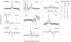 |
Fig. 2 Examples of NRT H I line profiles, showing flux density, SHI, in Jy as a function of radial velocity in the LSR frame, VLSR, in km s−1. The three vertical black lines indicate, respectively, the mean velocity and ± the expansion velocity of the CO line of each source. The sources shown here were classified as either clear H I detections (upper row), upper limits (middle row) or confused (lowest row). The spectra were obtained in position-switching mode for different east-west offset distances between the two off-source positions (throw amplitudes) located symmetrically around the on-source position. For the match between throw amplitudes and types of plotted lines used, we refer to the legend on the right-hand side. Throws are given in both units of the telescope’s east-west beam size (4′) and in arcminutes. The flat black horizontal lines show the 0 Jy flux density level. Also shown (as full black lines, with a shape distinctly different from the position-switching profiles) are the on-source H I profiles obtained in frequency-switching mode, with flux densities divided by a factor of 100. The frequency-switching mode observations were used as a benchmark for the overall confusion level throughout the spectra induced by the telescope’s near side lobes. For detections an increase of the total flux with throw amplitude indicates that the source is extended and the throw amplitude where the flux converges can be used to estimate the source diameter (see Sect. 3). |
3.2 Total H I profiles and source sizes
As noted above, in the case of a clear, strong detection of H I in a CSE, the H I profile converges once the throw amplitude is increased beyond the angular size of the CSE. When we indicate that the spectra of a target converge for spectrum CnEW, that is, at a throw amplitude of n HPBWs to the east and west of the target position C, this means the following:
the maximum line flux is reached in this spectrum;
the line flux remains the same for larger throw amplitudes (i.e. in spectra Cn+1EW, etc.);
there is therefore no CSE H I emission beyond a throw amplitude of n − 1 HPBWs from the star. Spectrum Cn − 1EW is the last to lie within the CSE, and the distances between the target star and the outer edges of beam positions Cn − 1E and Cn − 1W provide us with an estimate of the CSE diameter (see below).
We have therefore defined two types of spectra for the measurement of H I properties of CSEs, the ‘peak profile’ and the ‘total profile’. For practical reasons, the determination of the peak profile is different for strong detections and for weaker, spatially resolved detections (see below), whereas the total profile can only be determined for strong detections, whose names are flagged with aT in Tables B.2 and B.3.
We note that for the determination of both peak and the total profiles we have used only spectra obtained using east-west off-source positions with the same declination as the on-source position of the central star. We did not use the profiles obtained pointing north and south of the star (see Sect. 3.1).
Strong detections. For cases where there is a clear convergence for spectrum CnEW, obtained with a throw amplitude of n HPBWs, we define this as the peak profile (P). Additionally, we define a total profile (T) as the spectrum that contains all H I emission within a throw amplitude of n − 1 beams, which corresponds to the CSE size.
The relation between the total profile and the peak profile is (cf. Fig. 1)
 (1)
(1)
Using the following relation between the peak profile and the profiles at throw amplitudes of n HPBWs
 (2)
(2)
Equation (1) can be rewritten as follows:
 (3)
(3)
The diameter of the source is then (8n-4) arcmin, as the last profile that lies within the CSE, Cn-1EW, samples the H I out to a distance of ±(4n-2) arcmin from the on-source position (see Fig. 1).
To give an example (see Fig. 1): if the maximum is reached in profile C3EW, with a throw amplitude of 12′, then T = 5P − 2(C 1EW+C2EW), and the source diameter is 20′, that is, the maximum separation between outer edges of the HPBWs at off-source positions C2E and C2W.
Weaker detections. When there was no obvious convergence towards a maximum line flux, we use as peak profile P the average of all observed CnEW spectra (where n is an integer), in order to increase the signal-to-noise ratio of the profile. Here, we averaged the spectra, as adding them increases the noise level and makes weak detections invisible.
For an unresolved source this definition of the P profile is the same as given above for strong detections. However, we note that for spatially resolved weak sources it provides a lower limit to the aforementioned peak profile P. Also, for weak detections, which can only be seen in averaged spectra, no estimate can be made of the CSE’s angular diameter. For example, diameters could only be determined for 5 of the 21 possible detections (see Table B.4).
Details of the determination of H I profiles for selected sources are given in Appendix A.
 |
Fig. 3 Clear detections (we note that only the first four spectra are shown here; the full set is available in Appendix B). Shown is the flux density of the 21-cm H I line emission, SHI, in Jy, as a function of the radial velocity in the LSR reference frame, VLSR, in km s−1. The peak profiles (see Section 3.2) are indicated by solid black lines, while the total profiles are indicated by dashed black lines. The Gaussians fitted to the profiles are shown as blue lines, solid for fits to the peak profiles and dashed for fits to the total profiles. Spectra are shown for all 34 objects with clear H I detections (see Table B.2). The vertical black lines indicate the centre velocity of our Gaussian fit to the total H I profile (or, if not available, to the peak H I profile), the red vertical and horizontal lines show respectively the central CO or OH line velocity from the literature and its corresponding expansion velocity, whereas green lines indicate other types of literature velocities (e.g. optical or SiO lines) and an indicative expansion velocity of 10 km s−1, that is, the average measured value. The flat blue horizontal lines show the 0 Jy flux density level. The plotted total velocity range of all spectra is 60 km s−1. |
4 Results
We have classified the NRT H I line profiles as either clear detections, possible detections, or upper limits. Distinguishing between clear and possible detections can be a complex process, and is necessarily somewhat subjective, as it is based on various factors such as obscuration by (strong) Galactic H I lines, low signal-to-noise ratio, offset between H I and CO (or optical) line velocities, indication of confusion by a Galactic H I source along the line of sight. For each of the possible detections the reasons for which it has been classified as such are listed in Appendix A.
Basic, non-H I properties of the objects in our sample are given in Table B.1 for those with clear detections of their circumstellar H I emission, in Table B.3 for possible detections, in online Table 5 for objects with upper limits to their H I nondetections, and in online Table 6 for those whose CSE spectra are completely obscured by Galactic lines.
For objects with clear NRT detections results of our H I observations are given in Table B.2 and our spectra are shown in Figures 3 and B.1, for our possible detections the NRT results are listed in Table B.4 and spectra are shown in Figs. 4 and B.2, and for objects with upper limits the NRT results are listed in online only Table 5 and spectra are shown in Figs. 5 and B.3, but only for objects for which digital spectra are available, for example, those observed after the major NRT renovation in 2001 (see Sect. 3).
We fitted Gaussians to the H I profiles measured at the NRT and this was found to provide a good representation of the line shape. The same was done with VLA global H I profiles (see, e.g. Matthews et al. 2013). A Gaussian shape is expected in case of optically thin gas in an outflow that is slowed down in the outer parts of a CSE by interaction with the surrounding ISM; see, e.g. Le Bertre & Gérard (2004), Libert et al. (2007), and Matthews et al. (2013).
Our H I radial velocities were measured in the same local standard of rest (LSR) reference frame defined based on a solar motion of v⊙ = 20 km s−1 towards its apex at (B1950.0) α = 270.°5, δ = 30° (Kerschbaum & Olofsson 1999). The same conversion was applied to convert all published heliocentric velocities cz to the VLSR values listed in the Tables.
Measured radial velocities of evolved stars can vary significantly depending on the spectral lines used. For each object only one LSR velocity taken from the literature (V lit.) is given in the Tables. Our order of preference for listing velocities is (1) mm- wave CO lines, (2) maser lines (OH 1612 MHz, H2O, SiO), and (3) optical lines – as available.
Mass loss rates, Ṁ in M⊙ yr−1, are based on CO line modelling (see the references for Mref in the Tables), scaled to our adopted distance d.
The H I peak flux densities, Speak, and integrated line fluxes, FHI, listed in Tables B.2 and B.4 are those of the total H I profiles in the case of strong detections, which are flagged with aT after their names in the Tables, and of the peak H I profiles for weaker detections, which are flagged with aP in the Tables (see Sect. 3.2 for details). For the upper limit cases, all flux density limits listed in online Table 5 are for peak H I profiles.
The total H I masses, in M⊙, were calculated using the standard formula MHI = 2.356 ⋅ 10−7 d2 FHI, where the integrated H I flux FHI is in Jy km s−1 and distance d is in pc (see, e.g. Kellermann & Verschuur 1988).
Listed in Tables B.1–B.4 are the elements listed hereafter. We note that Table 5, listing the results for objects with upper limits to their NRT H I line signals, and Table 6, listing objects with confused NRT H I spectra, are available online only (see below).
In Table B.1 (clear NRT H I detections: basic data) and Table B.3 (possible NRT H I detections: basic data):
Name: common catalogue name of the target. An n after a name indicates that it is clearly not an AGB star, ad that we consider its classification as an AGB to be dubious, and a⋆ indicates that notes on the object can be found in Appendix A.
RA, Dec: literature right ascension and declination of the target from Gaia EDR 3 (Gaia Collaboration 2020), for epoch J2000.0;
Type: target type. Primarily the variability type as listed in Version 5.1 of the General Catalogue of Variable Stars, GCVS (Samus’ et al. 2017)1, but if an object is not included in the GCVS, other identifiers are listed in brackets: HPM = high proper motion star, (OH/IR) = OH/IR maser, LPVc = long period variable candidate, PN = planetary nebula, pPN = proto-planetary nebula, and post-AGB star;
Spec. & ref.: spectral type of the star, followed by its literature reference, as retrieved from the SIMBAD database. If none was listed there, the reference is noted as ‘SIMBAD’;
Teff & ref.: effective temperature of the star, in K, followed by its literature reference;
d: distance of the target, based on its parallax (mainly from the Gaia EDR3, Gaia Collaboration 2020), in pc. If no Gaia parallax was available a reference to the distance we adopted is given in Appendix A;
V lit.: published radial velocity of the target in the LSR reference frame, in km s−1 ;
Vexp : literature expansion velocity measured from CO or OH 1612 MHz line observations, in km s−1. If a pair of values was published for a two-velocity component CO line fit, the largest value is listed here;
ref.: literature references to the published V lit. and Vexp values;
line: spectral line on which the published radial velocity measurement (V lit.) was based;
Ṁ & ref.: literature mass loss rates, in M⊙ yr−1 , followed by its literature reference.
In Table B.2 (clear NRT H I detections:H I data) and Table B.4 (possible NRTH I detections: H I data):
Name: as in Table B.1;
VHI : our central radial velocity in the LSR reference frame of the Gaussian fitted to the H I profile, in km s−1 ;
FWHM: our full width half maximum of the Gaussian fitted to the H I line profile, in km s−1 ;
Speak : our peak flux density of the H I line profile, in Jy;
diam.: our estimated angular size of the H I CSE in the eastwest direction, in arcmin;
FHI : our integrated line flux of the H I profile, in Jy km s−1;
MHI : our total H I mass, in M⊙ ;
H I ref.: references to previously published H I studies.
Shown in Figures B.1, B.2 and B.3 are all spectra obtained with the renovated NRT for, respectively, the 34 clear detections, the 21 possible detections, and for the 70 objects for which an upper limit to its H I emission could be determined from digital versions of observations, that is, those observed from 2001 onwards with the renovated NRT (thus excluding the 25 objects with the ‘old data’ note in online Table 5). The peak profiles (see Section 3.2) are indicated by a solid black line, while the total profiles are indicated by a dashed black line. Also shown are the Gaussians fitted to each H I profile.
The short vertical black line indicates the centre velocity of our Gaussian fit to the total profile, or to the peak profile for weaker detections, and the short vertical red line the VLSR value taken from the literature, see Tables B.2 and B.4, and in online Table 5. The horizontal red line indicates the CO or OH line expansion velocity (if available – if not, the average expansion velocity of ±10km s−1 is indicated in green).
There is one object (RU Crt) without any published radial velocity. We have listed it among the confused sources, as we could not identify any obvious CSE H I emission from it, nor put an upper flux density limit to it.
 |
Fig. 4 Possible detections (we note that only the first four spectra are shown here; the full set is available in Appendix B). Shown is the flux density of the 21-cm H I line emission, SHI, in Jy, as a function of the radial velocity in the LSR reference frame, VLSR, in km s−1. The peak profiles (see Section 3.2) are indicated by a solid black line, while the total profiles (which could only be determined for GY Aql and U CMi) are indicated by a dashed black line. The Gaussians fitted to the profiles are shown as blue lines, solid for fits to the peak profiles and dashed for fits to the total profiles. Spectra are shown for all 21 objects with possible H I detections (see Table B.4). The vertical black lines indicate the centre velocity of our Gaussian fit to the peak H I profile (or, if available, to the total H I profile), the red vertical and horizontal lines show respectively the central CO or OH line velocity from the literature and its corresponding expansion velocity, whereas green lines indicate other types of literature velocities (e.g. optical or SiO lines) and an indicative expansion velocity of 10 km s−1, that is, the average measured value. The flat blue horizontal lines show the 0 Jy flux density level. The plotted total velocity range of the spectra is 60 km s−1, except for the 80 km s−1 range used for RAFGl 3099 due to its broad profile. |
 |
Fig. 5 Upper limits (we note that only the first four spectra are shown here; the full set is available in Appendix B). Shown is the flux density of the 21-cm H I line emission, SHI, in Jy, as a function of the radial velocity in the LSR reference frame, VLSR, in km s−1. All spectra are peak profiles (see Section 3.2). Spectra are shown only for the 70 objects with upper limits to their H I line emission for which digital versions of the observations are available, that is, those observed from 2001 onwards with the renovated NRT (thus excluding the 25 objects with the ‘old data’ note in online Table 5). The red vertical and horizontal lines indicate respectively the central CO or OH line velocity from the literature and its corresponding expansion velocity, whereas green lines indicate other types of literature velocities (e.g. optical or SiO lines) and an indicative expansion velocity of 10 km s−1, that is, the average measured value. The flat blue horizontal lines show the 0 Jy flux density level. The plotted total velocity range is the full observed range for each object. |
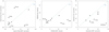 |
Fig. 6 Comparison of the results of the NRT and VLA HI line observations. Left: integrated line flux, FHI, in Jy km s−1; centre: FWHM width of the integrated line profile, in km s−1 ; right: source diameter, in arcmin. The diagonal lines marked with “1:1” indicate equality between the NRT and VLA measurements and were added to guide the eye only, but do not represent fits to the data. |
5 Discussion
Of the 290 observed objects, within the NRT beam clear H I detections of their CSE were made of 34 objects (11%), possible detections of 21 objects (7%) and upper limits to their H I mass could be determined for 95 objects (36%), whereas for 140 objects (46%) no conclusion could be drawn on their H I mass due to confusion by Galactic H I emission. For 33 detections the total H I flux and the size of the CSE could be determined.
Overall, the central velocities of our Gaussian fits to the H I profiles agree well with the CO line and optically determined velocities. For the 34 clear detections the mean difference ∆VLSR = −0.2 ± 2.0 km s−1 between CO and H I line velocities, and 0.8 ± 5.3 km s−1 between optically determined and H I velocities; and the difference between CO and optically- determined velocities is -2.2±3.4 km s−1 – if we ignore the two objects with optical values incompatible (∆VLSR ≥ 20km s−1) with several other reported values, R Cas (Vopt= −15 km s−1, from Famaey et al. 2005) and TX Psc (Vopt= −9.2 km s−1, from Wilson 1953), and the one with a large reported uncertainty, NGC 7293 (±10 km s−1, from Wilson 1953).
Since H I and CO emission lines originate in quite different regions of CSEs their profile shapes and widths cannot be compared directly. However, the H I lines seem to be narrower than the CO lines.
For the following 15 objects our present classification as either detection, upper limit or confused is different from those we gave in previous publications (see Appendix A for details on individual objects). This difference is due to the analysis of many more, and different types of, observations made at the NRT in subsequent years. We have sorted them into five categories, according to the differences between the new and old confusion and detection assessments. In three cases the classification was upgraded to detection or possible detection, whereas the other 12 cases were downgraded to either possible detection, upper limit or confused:
IRC +10216: confused, was detection; see Le Bertre & Gérard (2001), Matthews & Reid (2007) and Matthews et al. (2015);
NGC 6369: possible detection, was detection; see Gérard & Le Bertre (2006);
RAFGL 3068: upper limit, was detection; see Gérard & Le Bertre (2006);
RAFGL 3099: possible detection, was upper limit; see (Gérard & Le Bertre 2006) and Matthews et al. (2013);
W And: confused, was detection; see Gérard et al. (2011);
EP Aqr: possible detection, was detection; see Le Bertre & Gérard (2004) and Matthews & Reid (2007);
R Aqr: clear detection, was non-detection; see Matthews & Reid (2007);
S CMi: possible detection, was detection; see Gérard & Le Bertre (2006);
U CMi: possible detection, was detection; see Gérard & Le Bertre (2006);
Z Cyg: possible detection, was upper limit; see Gérard & Le Bertre (2006);
α1 Her: upper limit, was detection; see Gérard & Le Bertre (2006);
OP Her: upper limit, was detection; see Gérard et al. (2011);
δ02 Lyr: confused, was detection; see Gérard & Le Bertre (2006);
α Ori: confused, was detection ; see Bowers & Knapp (1987) and Le Bertre et al. (2012);
ρ Per: upper limit, was detection; see Gérard & Le Bertre (2006).
We compared (see Fig. 6) the global H I line profile parameters measured at the NRT and the VLA for the ten objects detected with both telescopes (see Sect. 1): o Cet, R Cas, RS Cnc, Y CVn, X Her, RX Lep, R Peg, TX Psc, V1942 Sgr, and Y UMa. The central line velocities are in good agreement, with an average NRT-VLA difference of 0.3 ± 0.5 km s−1, cf. the typical uncertainty of ∼0.15 km s−1 for the VLA profiles. When comparing the measured line fluxes and FWHMs, some objects show a notable difference between their NRT and VLA values.
Considerably higher line fluxes measured with the NRT could, in principle, be ascribed to low-column density, extended H I structures within a CSE, which remained below the VLA detectability threshold but were detectable with the larger NRT beam (for X Her). On the other hand, this effect could not explain the considerable higher line fluxes measured with the VLA (for R Cas, RX Lep, and TX Psc). For these objects the discrepancies may rather be due to the rather different methods used to separate CSE line emission from ambient Galactic lines in VLA and NRT data.
We note that in three objects with discrepant line fluxes the line FWHMs are also significantly different (R Cas, X Her and RX Lep). For Y UMa we used the single component H I line parameters which we determined from the global VLA profile published by Matthews et al. (2013), who fitted two components to their profile (see Appendix A for further details).
R Cas: the VLA line flux (Matthews & Reid 2007) is seven times lower than our NRT value of 0.6 Jy km s−1 and the VLA F WHM is four times smaller than the NRT value of 12 km s−1. The source diameters are similar, 13.′4 (VLA) and ∼12′ (NRT). Both NRT and VLA detections are faint, at, respectively, MHI = 0.00063 and 0.00047 M⊙. The VLA-NRT discrepancy may simply be due to the low signal-to-noise ratios in both observations.
X Her: the VLA line flux Matthews et al. (2011) is 11 times lower than our NRT value of 1.2 Jy km s−1 and the VLA F WHM is three times smaller than the NRT value of 15 km s−1. The H I cartography by Matthews et al. (2011) of X Her and its surroundings with the VLA and the GBT revealed the presence of a nearby, compact HVC cloud seen in superposition on the CSE emission of X Her, which they named Cloud I. The VLA–NRT discrepancy is likely due to confusion with Cloud I – see also the discussion in Matthews et al. (2011).
RX Lep: the VLA line flux (Matthews et al. 2013) is 2.4 times higher than our NRT value of 1.2 Jy km s−1, which is the same as the NRT value from Libert et al. (2008), and the VLA FWHM is 1.7 times larger than our NRT value of 2.9 km s−1. As noted by Matthews et al. (2013), the reason for the discrepancy is unclear, but may be partly due to the different methods used to separate CSE and surrounding Galactic signals in VLA and NRT data;
TX Psc: the VLA line flux Matthews et al. (2013) is 3.3 times higher than our NRT value of 0.45 Jy km s−1 and the VLA FWHM is 1.2 times larger than the NRT value of 3.2 km s−1. The VLA data show the presence of large, nearby H I structures which are also close in velocity to the CSE emission from TX Psc, but which do not appear to be related to the target star. The VLA-NRT discrepancy is likely due to the presence of these Galactic clouds – see also Matthews et al. (2013).
Concerning the diameters of the NRT clear detections, eight sources were unresolved, with diameters <4′, and the diameters of the 26 resolved sources range from 4′ to 44′, with an average of 20′ ± 10′. We could compare these values with source diameters measured with the VLA for seven objects. For four (R Cas, RX Lep, R Peg, TX Psc) the diameters are comparable, the NRT diameter is about twice as large for two others (Y CVn and Y UMa), and for V1942 Sgr the NRT diameter is six times larger.
6 Conclusions
A search was carried out during the past 30 years for H I line emission from circumstellar envelopes (CSEs) of mass-losing asymptotic giant branch stars and other types of evolved stars. Such observations can, for example, trace gas far outside the CO dissociation radius, and probe the interface between the star and the interstellar medium.
Using the single-dish NRT, total H I masses could be measured for CSEs, and for clear detections their east-west sizes could be estimated. Of the 290 targets, 34 were clearly detected, 21 had possible detections, for 95 an upper limit to their H I line emission could be determined, and for 140 objects no conclusion could be drawn about their H I content due to confusion with surrounding Galactic H I clouds.
Of the 37 miras with digital spectra, 22% have clear H I detections; whereas of the 54 SR types, 35% have clear detections. The total H I masses of the clearly detected AGB stars cover a wide range of about a factor 150, from ∼0.001 to 0.15 M⊙. The different types of AGB stars all cover about the same range.
The linear east-west diameters of the 28 resolved H I sources as determined with the NRT cover a range of a factor 30, from 0.17 to 5.2 pc, with an average of 1.6 ± 1.4 pc. The ten unresolved sources have upper limits ranging from 0.5 to 2.6 pc (average 1.0 ± 0.8 pc). On average, the radii of the 21 resolved miras and SR-type AGBs are comparable, 1.0 ± 0.8 pc and 1.4 ± 1.2 pc, respectively. The two outliers with a large H I diameter of order 5.2 pc are RY Dra (SRb:) and V1942 Sgr (Lb).
The stars in our sample cover two orders of magnitude for the mass-loss rate, from about 0.2 to 20 10−7 M⊙ yr−1. There is no clear overall trend of H I or CO line widths with the mass-loss rate.
We will present an analysis of our H I results in a future study, Gérard et al. (in prep., Paper II). In it, we will focus on the differences in atomic and molecular hydrogen masses of AGB CSEs.
Data availability
All six tables are available online, Tables B.1 to B.4, as well as online only Table 5, with the results for objects with upper limits to their NRT H I line signals, and online only Table 6, with the objects with confused NRT H I spectra (https://doi.org/10.5281/zenodo.14050100).
Acknowledgements
This paper is dedicated to the memory of Nguyên Quang Riêu, who initiated this research. We wish to thank the staff of the Nançay Radio Telescope for their support with the observations over the past 30 years. The Nançay Radio Observatory is operated by the Paris Observatory, associated with the French Centre National de la Recherche Scientifique. This research has made use of the SIMBAD database, operated at CDS, Strasbourg, France. L.D.M. was supported by award AST-2107681 from the National Science Foundation.
Appendix A Notes on individual objects
Objects are listed first in order of their catalogue name (IRC, NGC and RAFGL), and then in alphabetical order of their constellation’s name. Stars which are clearly not AGBs are denoted by an n after their name and those for which we consider their classification as AGB dubious are denoted by a d .
IRC -10529: We adopted the distance of 270 pc used by Ramstedt et al. (2020) as it has no parallax listed in the Gaia EDR3.
IRC +10216: We now consider the NRT H I observation to be confused by a source located at an off-source position. It was previously classified as an NRT detection in absorption by Le Bertre & Gérard (2001), which the VLA imaging by Matthews & Reid (2007) showed to be a likely artefact due to H I emission detected with the VLA within an NRT off-source reference beam. However, subsequent imaging with the 100m Green Bank Telescope (Matthews et al. 2015) revealed a low surface brightness H I shell of about 20′ (0.8 pc) size centred on the star.
NGC 6369n : Listed previously as a detection in Gérard & Le Bertre (2006), we classified this planetary nebula as a possible detection, due to the low signal-to-noise ratio of its broad (FWHM = 36 km s−1) H I profile.
RAFGL 865: We adopted the distance of 1580 pc used by Menzies et al. (2006) as it has no parallax listed in the Gaia EDR3.
RAFGL 3068: Classified as an upper limit, whereas it was previously listed as a detection in Gérard & Le Bertre (2006). We adopted the distance of 980 pc used by Andriantsaralaza et al. (2021) as it has no parallax listed in the Gaia EDR3. It is an AGB star transitioning towards the proto-Planetary Nebula phase (Kim et al. 2017).
RAFGL 3099: Listed previously as an NRT upper limit by Gérard & Le Bertre (2006) and as a VLA non-detection by Matthews et al. (2013), both with a ∼2 mJy limit. After 100 hours of NRT observations we classified this very low signal-to-noise H I signal as a possible detection, with an H I peak flux density of ∼7 mJy at the upper edge of the CO line FWHM. The average flux density we measured within the Gaussian profile fit is 2±2 mJy, the same as the previous NRT and VLA upper limit levels. We adopted the distance of 2100 pc from Knapp & Morris (1985) as it has no parallax listed in the Gaia EDR3.
W And: Classified as confused, whereas it was previously classified as a detection in Gérard et al. (2011).
56 Aqln: Classified as a possible detection due to the low signal-to-noise ratio of the H I profile, and the 6.4 km s−1 difference between the H I and optical velocities; the optical velocity has a published uncertainty of 2 km s−1 in the GCRV (Wilson 1953).
GY Aql: Classified as a possible detection, as it lies on the edge of strong Galactic H I lines, which obscure the lower half of the CO profile width. The NRT H I profile parameters are bound to be underestimates, and no diameter could be estimated. Although we could determine a total H I profile, it is quite different from the peak profile.
EP Aqr: Classified as a possible detection, whereas it was previously listed as an NRT detection by Le Bertre & Gérard (2004) and as a VLA detection by Matthews & Reid (2007), where arcminute-scale H I structures were observed which were offset from the star’s position by up to 10′. There could be two components in the NRT profile, but we have fitted only a single Gaussian.
R Aqrd: Classified as a clear detection. Matthews & Reid (2007) did not detect an H I source at the position of the continuum source, but do not exclude possible spatially extended H I emission. It is a symbiotic star, a binary system with a mira and a white dwarf.
RW Boo: This is the only clear NRT detection with a significant difference of 15 km s−1 between our H I velocity of 10.1 km s−1 and the CO velocity of −5.0 km s−1 published by Díaz-Luis et al. (2019). However, the CO line profile shows that their published central velocity of −5.0 km s−1 lies on the lower edge of the profile, whereas we estimate the central velocity as 6 km s−1. The published CO expansion velocity of 34.6 km s−1 is in fact the FWHM of the line profile, so twice as large as our definition of Vexp, whereas the FWHM we estimate from their spectrum is only 18 km s−1. We therefore listed a literature velocity (V lit.) of 6 km s−1 and a Vexp of 9 km s−1 in Table B.1.
µ Cepn: We adopted the distance of 641 pc determined by Montargès et al. (2019) as it has no parallax listed in the Gaia EDR3. Our H I detection of this red supergiant, which is centred on 38 km s−1, only shows the high-velocity half of the CO line profile; the lower part is confused by strong Galactic H I signals. The single-dish CO(4-3) line profile by De Beck et al. (2010) is centred on ∼33 km s−1, with a large FWHM of ∼65 km s−1. The NOEMA interferometric CO(2-1) line imaging by Montargès et al. (2019) shows a clumpy CO distribution, with emission in the range −8 to 58 km s−1. A high-resolution optical spectrum obtained by Montargès et al. (2019) shows that the radial LSR velocity of the central star is 32.7 km s−1.
T Cep: Ramstedt et al. (2009) noted that all six of their CO line profiles were asymmetric, with stronger emission on the red side. They saw this as an indication of an asymmetric outflow, as the lines are all optically thin.
T Cet: The total profile shows a strong peak at 19 km s−1 which is not present in the peak profile; it remains to be seen if it is associated with the CSE.
S CMi: Listed previously as a detection in Gérard & Le Bertre (2006), whereas we have classified it as a possible detection, unresolved by the NRT, as the new observations made pointing 11′ north and south of the star indicate there may be confusion by ISM H I emission along the line of sight.
U CMi: Listed previously as detection in Gérard & Le Bertre (2006) and as possible detection here; the case for possible confusion needs to be investigated further. We could however measure a total H I profile for the detection.
RS Cnc: As the C 1EW and C2EW profiles are rather similar we used the averaged spectrum for further analysis, and conclude that the source diameter is 4′. VLA H I observations Matthews & Reid (2007) show a compact (80″ diameter) source centred on the star plus a 6′ long filament.
W Cnc: Classified as a possible detection due to the low signal-to-noise ratio of the H I profile.
T Com: Classified as a possible detection due to confusion by Galactic H I at the lower-velocity end of the profile.
Y CVn: It has the highest measured signal-to-noise ratio among our H I CSE detections. We have listed its diameter as 16′ as the east-west profiles first converge at a throw amplitude of 8′, but there is an indication of a weak extension out to 12′ radius, suggesting a faint envelope between 6′ and 10′ radius. The profile is clearly asymmetric with an excess on its low-velocity side that is present down to 6.5 km s−1 in both the peak and total profiles.
Z Cyg: Previously listed as an upper limit in Gérard & Le Bertre (2006), we classified it as a possible detection as the low signal-to- noise H I signal is centred exactly on the CO line detection by Josselin et al. (1998). The fitted H I line width (FWHM = 17: km s−1) is considerably broader than that of the CO line (9 km s−1 ), but the Gaussian fit is not very precise due to the weakness of the line signal.
AH Dra: Classified as a possible detection as it has a quite low signal-to-noise ratio.
S Dra: Classified as a possible detection as it has a low signal-to-noise ratio, and as its lower-velocity edge may be contaminated by Galactic H I.
UX Dra: Classified as a possible detection as its lower-velocity half may be contaminated by Galactic H I.
RY Dra: The source is very extended, with an estimated diameter of 44′, in agreement with the far-infrared IRAS source size measured at 60 and 100 µm wavelength by Young et al. (1993).
α1 Herd : Classified as an upper limit, whereas it was previously classified as a detection in Gérard & Le Bertre (2006). We adopted the distance of 110 pc based on its HIPPARCOS parallax (van Leeuwen 2007) as it has no parallax listed in the Gaia EDR3.
OP Her: Classified as an upper limit, whereas it was previously classified as a detection in Gérard et al. (2011).
X Her: There is a hint of two Gaussian components in the spectrum, but we made a fit using only one Gaussian.
U Hya: Although it is an SRb carbon star, like Y CVn, their mass loss histories appear to be very different, in the sense that U Hya has a 50 times smaller H I mass and that the 2′ radius detached ring seen in the far-infrared maps of Cox et al. (2012a) and Cox et al. (2012b) is most likely due to a short episode of enhanced mass-loss rate (Waters et al. 1994).
W Hya: Classified as confused, whereas it was previously classified as a detection in Gérard & Le Bertre (2006). No H I was detected by Hawkins & Proctor (1993) in VLA imaging observations with an rms noise level of 0.0055 Jy/beam.
AF Leo : As the maximum is almost reached at C2EW but the C2EW spectrum is a bit higher, we estimate its diameter as 16′. As peak profile we used the average of the C3EW and C4EW spectra.
δ02 Lyrd : Classified as confused, whereas it was previously classified as detected in Gérard & Le Bertre (2006).
α Orin : We now consider the NRT H I observation of this red supergiant to be confused, whereas it was previously classified as a detection based on a VLA detection by Bowers & Knapp (1987) and on detections with both NRT and VLA by Le Bertre et al. (2012) which shows a detached H I shell of about 4′ diameter.
SV Peg: Classified as a possible detection as the profiles do not converge well. Furthermore, the lower-velocity edge of the CO profile width is contaminated by strong Galactic H I.
V Peg: We adopted the distance of 1380 pc used by Benson & Little-Marenin (1996) as the Gaia EDR3 parallax is very uncertain, 0.022±0.092 mas
ρ Perd : Classified as an upper limit, whereas it was previously classified as a detection in Gérard & Le Bertre (2006).
SV Psc: As the C 1EW to C4EW spectra are similar we used the averaged spectrum for further analysis, and conclude that the source is unresolved. Winters et al. (2003) noted that both their CO line profiles show two components with different outflow velocities, of 2 and 11 km s−1, respectively. The mass loss rate of 1.0 10−6 M⊙ yr−1 we listed in Table B.1 is for the broader component.
TX Psc: Imaging observations with the VLA by Matthews et al. (2013) identified Galactic H I confusion in the 7-8 km s−1 VLSR range, a line signal which had contaminated the NRT spectra of Gérard & Le Bertre (2006). Separating genuine CSE emission from the confusing emission feature is difficult in the NRT data. When using throw amplitudes up to 4′ (C1EW), we observe an H I line centred on 12 km s−1 , in agreement with the VLA detection of the CSE. As the NRT spectra converge between C1.5EW and C2.5EW we estimate its diameter as 8′, which is larger than the 6.′2 measured at the VLA, but this may be due to the confusing line signal which increases for larger throw amplitudes.
WX Psc: We adopted the distance of 740 pc used by van Langevelde et al. (1990) as it has no parallax listed in the Gaia EDR3.
Y Scl: We have classified this clear H I line as a possible detection due to the 4 km s−1 difference between the H I and CO line velocities, which is significant when compared to the CO line FWHM of 14.6 km s−1 (Kerschbaum & Olofsson 1999).
κ Sern : Classified as a possible detection as the upper edge of the H I profile is contaminated by strong Galactic H I.
S Ser: Classified as a possible detection as the lower-velocity half of the H I profile is contaminated by Galactic H I, and as it is much narrower (FWHM = 2.6 km s−1) than the average 20 km s−1 FWHM line width of the CO line detections of our sample (no CO line detected has been published of the source).
WX Ser: Classified as a possible detection on the edge of strong Galactic H I lines, which obscure the lower-velocity 60% of the CO profile width. The NRT H I profile parameters are bound to be underestimates, and no diameter could be estimated.
AQ Sgr: Classified as a possible detection, and estimate its diameter as 4′. NRT observations show the presence of a confusing source to the north which appears around 18 km s−1, that is, about 2.5 km s−1 lower than the profile peak velocity, and which may cause the asymmetry in the profile shown here. However, the confusion appears negligible out to east-west throw amplitudes of 6′ and is only clearly present at 10′.
V1942 Sgr: High signal-to-noise source that was studied previously with the NRT and VLA Matthews et al. (2013). It was observed with throw amplitudes from 1.3′ to 48′. The spectra start to converge at C 1.5EW (source diameter of 8′), but there appears to be H I out to a diameter of 28′. We do not find evidence in our NRT spectra for the previously reported (Libert et al. 2010a) H I emission pedestal between −29 and −37 km s−1 at the ∼6 mJy level, and neither did Matthews et al. (2013) in their VLA observations. The non-detection of the broad component is not surprising given the rms noise levels in the VLA data and our NRT spectra (3.6 mJy for our peak spectrum and 27 mJy for our total spectrum).
IK Tau: Not detected by either the VLA Matthews et al. (2013) with an rms of 1.4 mJy/beam nor at the NRT, with an rms of 3.7 mJy.
Y UMa: Matthews et al. (2013) fitted two components to their VLA H I profile. The first has a considerably smaller width and higher peak flux density. The fitted values for the components are, respectively: VHI = 16.4, 17.2 km s−1 ; FWHM = 3.2, 9.2 km s−1; Speak = 0.10, 0.03 mJy. We cannot discern the broader component in our NRT profile, which is not surprising as its VLA peak value is only 2.3 times the 0.013 Jy rms noise level of the NRT spectrum. We fitted only a single Gaussian to our NRT profile, with VHI = 16.8 km s−1 ; FWHM = 5.4 km s−1, and Speak = 0.10 Jy. These values agree well with the overall parameters which we determined from the VLA profile: VHI = 16.6 km s−1; FWHM = 4.9 km s−1, and Speak = 0.13 Jy.
V UMi: Classified as a possible detection as the H I profile has a low signal-to-noise ratio, and as it is considerable narrower (FWHM = 4.9 km s−1) than the average 20 km s−1 FWHM line width of the CO line detections of our sample (no CO line detected has been published of the source).
RW Vir: Classified as a possible detection as the C1EW to C4EW spectra do not converge well.
Appendix B NRT H I line spectra and tables
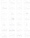 |
Fig. B.1 a. Clear detections. Shown is flux density of the 21-cm H I line emission, SHI, in Jy, as a function of radial velocity in the LSR reference frame, VLSR, in km s−1. The peak profiles (see Section 3.2) are indicated by solid black lines, while the total profiles are indicated by dashed black lines. The Gaussians fitted to the profiles are shown as blue lines, solid for fits to the peak profiles and dashed for fits to the total profiles. Spectra are shown for all 34 objects with clear H I detections (see Table B.2). The vertical black lines indicate the centre velocity of our Gaussian fit to the total H I profile (or, if not available, to the peak H I profile), the red vertical and horizontal lines show respectively the central CO or OH line velocity from the literature and its corresponding expansion velocity, whereas green lines indicate other types of literature velocities (e.g. optical or SiO lines) and an indicative expansion velocity of 10 km s−1, that is, the average measured value. The flat blue horizontal lines show the 0 Jy flux density level. The plotted total velocity range of all spectra is 60 km s−1. b. Clear detections |
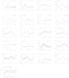 |
Fig. B.2 Possible detections. Shown is flux density of the 21-cm H I line emission, SHI, in Jy, as a function of radial velocity in the LSR reference frame, VLSR, in km s−1 . The peak profiles (see Section 3.2) are indicated by a solid black line, while the total profiles (which could only be determined for GY Aql and U CMi) are indicated by a dashed black line. The Gaussians fitted to the profiles are shown as blue lines, solid for fits to the peak profiles and dashed for fits to the total profiles. Spectra are shown for all 21 objects with possible H I detections (see Table B.4). The vertical black lines indicate the centre velocity of our Gaussian fit to the peak H I profile (or, if available, to the total H I profile), the red vertical and horizontal lines show respectively the central CO or OH line velocity from the literature and its corresponding expansion velocity, whereas green lines indicate other types of literature velocities (e.g. optical or SiO lines) and an indicative expansion velocity of 10 km s−1, that is, the average measured value. The flat blue horizontal lines show the 0 Jy flux density level. The plotted total velocity range of the spectra is 60 km s−1, except for the 80 km s−1 range used for RAFGl 3099 due to its the broad profile. |
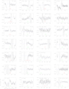 |
Fig. B.3 a. Upper limits. Shown is flux density of the 21-cm H I line emission, S HI, in Jy, as a function of radial velocity in the LSR reference frame, VLSR, in km s−1. All spectra are peak profiles (see Section 3.2). Spectra are shown only for the 70 objects with upper limits to their H I line emission for which digital versions of the observations are available, that is, those observed from 2001 onwards with the renovated NRT (thus excluding the 25 objects with the ’old data’ note in online Table 5). The red vertical and horizontal lines indicate respectively the central CO or OH line velocity from the literature and its corresponding expansion velocity, whereas green lines indicate other types of literature velocities (e.g. optical or SiO lines) and an indicative expansion velocity of 10 km s−1, that is, the average measured value. The flat blue horizontal lines show the 0 Jy flux density level. The plotted total velocity range is the full observed range for each object. b. Upper limits c. Upper limits |
Clear NRT H I detections: basic data
Clear NRT H I detections: H I data
Possible NRT H I detections: basic data
Possible NRT H I detections: H I data
References
- Allen, D. A., Hyland, A. R., Longmore, A. J., et al. 1977, ApJ, 217, 108 [NASA ADS] [CrossRef] [Google Scholar]
- Andriantsaralaza, M., Ramstedt, S., Vlemmings, W. H. T., et al. 2021, A&A, 653, A53 [NASA ADS] [CrossRef] [EDP Sciences] [Google Scholar]
- Baars, J. W. M., Genzel, R., Pauliny-Toth, I.I. K., & Witzel, A. 1977, A&A, 61, 99 [NASA ADS] [Google Scholar]
- Barnbaum, C., Stone, R. P. S., & Keenan, P. C. 1996, ApJS, 105, 419 [NASA ADS] [CrossRef] [Google Scholar]
- Benson, P. J., & Little-Marenin, I. R. 1996, ApJS, 106, 579 [NASA ADS] [CrossRef] [Google Scholar]
- Benson, P. J., Little-Marenin, I. R., Woods, T. C., et al. 1990, ApJS, 74, 911 [NASA ADS] [CrossRef] [Google Scholar]
- Bergeat, J., Knapik, A., & Rutily, B. 2001, A&A, 369, 178 [NASA ADS] [CrossRef] [EDP Sciences] [Google Scholar]
- Bidelman, W. P. 1954, ApJS, 1, 175 [NASA ADS] [CrossRef] [Google Scholar]
- Bidelman, W. P. 1980, Pub. Warner Swasey Obs., 2, 1 [Google Scholar]
- Bidelman, W. P., & MacConnell, D. J. 1973, AJ, 78, 687 [NASA ADS] [CrossRef] [Google Scholar]
- Bowers, P. F., & Knapp, G. R. 1987, ApJ, 315, 305 [NASA ADS] [CrossRef] [Google Scholar]
- Bowers, P. F., & Knapp, G. R. 1988, ApJ, 332, 299 [NASA ADS] [CrossRef] [Google Scholar]
- Bujarrabal, V., Bachiller, R., Alcolea, J., & Martin-Pintado, J. 1988, A&A, 206, L17 [NASA ADS] [Google Scholar]
- Cho, S.-H., & Kim, J. 2012, AJ, 144, 129 [CrossRef] [Google Scholar]
- Cho, S. H., Kaifu, N., & Ukita, N. 1996, A&AS, 115, 117 [NASA ADS] [Google Scholar]
- Cohen, M. 1979, MNRAS, 186, 837 [NASA ADS] [Google Scholar]
- Cohen, M., & Kuhi, L. V. 1976, PASP, 88, 535 [NASA ADS] [CrossRef] [Google Scholar]
- Cox, N. L. J., Kerschbaum, F., van Marie, A. J., et al. 2012a, A&A, 537, A35 [NASA ADS] [CrossRef] [EDP Sciences] [Google Scholar]
- Cox, N. L. J., Kerschbaum, F., van Marle, A. J., et al. 2012b, A&A, 543, C1 [NASA ADS] [CrossRef] [EDP Sciences] [Google Scholar]
- Danilovich, T., Teyssier, D., Justtanont, K., et al. 2015, A&A, 581, A60 [NASA ADS] [CrossRef] [EDP Sciences] [Google Scholar]
- De Beck, E., Decin, L., de Koter, A., et al. 2010, A&A, 523, A18 [NASA ADS] [CrossRef] [EDP Sciences] [Google Scholar]
- De Mello, A. B., Lorenz-Martins, S., de Araújo, F. X., Bastos Pereira, C., & Codina Landaberry, S. J. 2009, ApJ, 705, 1298 [NASA ADS] [CrossRef] [Google Scholar]
- Dean, C. A. 1976, AJ, 81, 364 [NASA ADS] [CrossRef] [Google Scholar]
- Decin, L. 2021, ARA&A, 59, 337 [NASA ADS] [CrossRef] [Google Scholar]
- Decin, L., Cherchneff, I., Hony, S., et al. 2008, A&A, 480, 431 [NASA ADS] [CrossRef] [EDP Sciences] [Google Scholar]
- Díaz-Luis, J. J., Alcolea, J., Bujarrabal, V., et al. 2019, A&A, 629, A94 [NASA ADS] [CrossRef] [EDP Sciences] [Google Scholar]
- Dumm, T., & Schild, H. 1998, New A, 3, 137 [CrossRef] [Google Scholar]
- Dyck, H. M., van Belle, G. T., & Thompson, R. R. 1998, AJ, 116, 981 [NASA ADS] [CrossRef] [Google Scholar]
- Evans, D. S. 1967, IAU Symp., 30, 57 [NASA ADS] [Google Scholar]
- Famaey, B., Jorissen, A., Luri, X., et al. 2005, A&A, 430, 165 [CrossRef] [EDP Sciences] [Google Scholar]
- Famaey, B., Pourbaix, D., Frankowski, A., et al. 2009, A&A, 498, 627 [NASA ADS] [CrossRef] [EDP Sciences] [Google Scholar]
- Feast, M. W., & Whitelock, P. A. 2000, MNRAS, 317, 460 [NASA ADS] [CrossRef] [Google Scholar]
- Feast, M. W., Woolley, R., & Yilmaz, N. 1972, MNRAS, 158, 23 [CrossRef] [Google Scholar]
- Feibelman, W. A. 1999, PASP, 111, 221 [NASA ADS] [CrossRef] [Google Scholar]
- Frasca, A., Molenda-Zakowicz, J., De Cat, P., et al. 2016, A&A, 594, A39 [CrossRef] [EDP Sciences] [Google Scholar]
- Frogel, J. A., Dickinson, D. F., & Hyland, A. R. 1975, ApJ, 201, 392 [NASA ADS] [CrossRef] [Google Scholar]
- Gaia Collaboration. 2020, VizieR Online Data Catalog: I/350 [Google Scholar]
- Gardan, E., Gérard, E., & Le Bertre, T. 2006, MNRAS, 365, 245 [NASA ADS] [CrossRef] [Google Scholar]
- Gérard, E., & Le Bertre, T. 2003, A&A, 397, L17 [NASA ADS] [CrossRef] [EDP Sciences] [Google Scholar]
- Gérard, E., & Le Bertre, T. 2006, AJ, 132, 2566 [CrossRef] [Google Scholar]
- Gérard, E., Le Bertre, T., & Libert, Y. 2011, in SF2A_2011: Proceedings of the Annual meeting of the French Society of Astronomy and Astrophysics, eds. G. Alecian, K. Belkacem, R. Samadi, & D. Valls-Gabaud, 419 [Google Scholar]
- Gianninas, A., Bergeron, P., & Ruiz, M. T. 2011, ApJ, 743, 138 [Google Scholar]
- Glassgold, A. E., & Huggins, P. J. 1983, MNRAS, 203, 517 [NASA ADS] [Google Scholar]
- Gontcharov, G. A. 2006, Astron. Lett., 32, 759 [Google Scholar]
- Granet, C., James, G. L., & Pezzani, J. 1999, J. Elec. Electron. Eng. Australia, 19, 111 [Google Scholar]
- Gray, R. O., Corbally, C. J., Garrison, R. F., McFadden, M. T., & Robinson, P. E. 2003, AJ, 126, 2048 [Google Scholar]
- Groenewegen, M. A. T., de Jong, T., & Gaballe, T. R. 1994, A&A, 287, 163 [NASA ADS] [Google Scholar]
- Groenewegen, M. A. T., Baas, F., Blommaert, J. A. D. L., et al. 1999, A&AS, 140, 197 [NASA ADS] [CrossRef] [EDP Sciences] [Google Scholar]
- Groenewegen, M. A. T., Sevenster, M., Spoon, H. W. W., & Pérez, I. 2002, A&A, 390, 511 [NASA ADS] [CrossRef] [EDP Sciences] [Google Scholar]
- Guo, Y. X., Luo, A. L., Zhang, S., et al. 2019, MNRAS, 485, 2167 [CrossRef] [Google Scholar]
- Hansen, O. L., & Blanco, V. M. 1975, AJ, 80, 1011 [NASA ADS] [CrossRef] [Google Scholar]
- Hawkins, G., & Proctor, D. 1993, in European Southern Observatory Conference and Workshop Proceedings, 46, 461 [NASA ADS] [Google Scholar]
- Herbig, G. H. 1960, ApJ, 131, 632 [NASA ADS] [CrossRef] [Google Scholar]
- Herbig, G. H. 1977, ApJ, 214, 747 [Google Scholar]
- Hoai, D. T., Matthews, L. D., Winters, J. M., et al. 2014, A&A, 565, A54 [NASA ADS] [CrossRef] [EDP Sciences] [Google Scholar]
- Hoai, D. T., Nhung, P. T., Matthews, L. D., Gérard, E., & Le Bertre, T. 2017, Res. Astron. Astrophys., 17, 67 [Google Scholar]
- Höfner, S., & Olofsson, H. 2018, A&A Rev., 26, 1 [CrossRef] [Google Scholar]
- Houk, N. 1982, Michigan Catalogue of Two-dimensional Spectral Types for the HD stars (Michigan: Department of Astronomy, University of Michigan), 3 [Google Scholar]
- Houk, N., & Smith-Moore, M. 1988, Michigan Catalogue of Two-dimensional Spectral Types for the HD Stars (Michigan: Department of Astronomy, University of Michigan), 4 [Google Scholar]
- Houk, N., & Swift, C. 1999, Michigan Catalogue of Two-dimensional Spectral Types for the HD Stars (Department of Astronomy, University of Michigan), 5 [Google Scholar]
- Huggins, P. J., & Healy, A. P. 1989, ApJ, 346, 201 [NASA ADS] [CrossRef] [Google Scholar]
- Humphreys, R. M. 1974, ApJ, 188, 75 [Google Scholar]
- Joint IRAS Science Working Group 1997, VizieR Online Data Catalog: III/197 [Google Scholar]
- Josselin, E., Loup, C., Omont, A., Barnbaum, C., & Nyman, L. A. 1996, A&A, 315, L23 [Google Scholar]
- Josselin, E., Loup, C., Omont, A., et al. 1998, A&AS, 129, 45 [NASA ADS] [CrossRef] [EDP Sciences] [Google Scholar]
- Joy, A. H. 1942, ApJ, 96, 344 [CrossRef] [Google Scholar]
- Jura, M., Kahane, C., & Omont, A. 1988, A&A, 201, 80 [NASA ADS] [Google Scholar]
- Kahane, C., & Jura, M. 1994, A&A, 290, 183 [NASA ADS] [Google Scholar]
- Kahane, C., Barnbaum, C., Uchida, K., Balm, S. P., & Jura, M. 1998, ApJ, 500, 466 [NASA ADS] [CrossRef] [Google Scholar]
- Keenan, P. C. 1942, ApJ, 95, 461 [NASA ADS] [CrossRef] [Google Scholar]
- Keenan, P. C. 1954, ApJ, 120, 484 [NASA ADS] [CrossRef] [Google Scholar]
- Keenan, P. C. 1966, ApJS, 13, 333 [NASA ADS] [CrossRef] [Google Scholar]
- Keenan, P. C. 1993, PASP, 105, 905 [Google Scholar]
- Keenan, P. C., & Boeshaar, P. C. 1980, ApJS, 43, 379 [NASA ADS] [CrossRef] [Google Scholar]
- Keenan, P. C., & McNeil, R. C. 1989, ApJS, 71, 245 [Google Scholar]
- Keenan, P., & Young, W. 1964, AJ, 69, 546 [NASA ADS] [CrossRef] [Google Scholar]
- Keenan, P. C., Garrison, R. F., & Deutsch, A. J. 1974, ApJS, 28, 271 [CrossRef] [Google Scholar]
- Kellermann, K. I., & Verschuur, G. L. 1988, Galactic and Extragalactic Radio Astronomy (New York: Galactic and Extragalactic Radio Astronomy) [Google Scholar]
- Kemper, F., Stark, R., Justtanont, K., et al. 2003, A&A, 407, 609 [NASA ADS] [CrossRef] [EDP Sciences] [Google Scholar]
- Kerschbaum, F., & Olofsson, H. 1998, A&A, 336, 654 [NASA ADS] [Google Scholar]
- Kerschbaum, F., & Olofsson, H. 1999, A&AS, 138, 299 [NASA ADS] [CrossRef] [EDP Sciences] [Google Scholar]
- Kharchenko, N. V., Scholz, R. D., Piskunov, A. E., Röser, S., & Schilbach, E. 2007, Astron. Nachr., 328, 889 [Google Scholar]
- Kim, J., Cho, S.-H., & Kim, S. J. 2013, AJ, 145, 22 [CrossRef] [Google Scholar]
- Kim, J., Cho, S.-H., & Kim, S. J. 2014, AJ, 147, 22 [Google Scholar]
- Kim, H., Trejo, A., Liu, S.-Y., et al. 2017, Nat. Astron., 1, 0060 [Google Scholar]
- Kim, J., Cho, S.-H., Oh, C. S., & Byun, D.-Y. 2010, ApJS, 188, 209 [NASA ADS] [CrossRef] [Google Scholar]
- Klochkova, V. G. 1997, Bull. Special Astrophys. Observ., 44, 5 [Google Scholar]
- Knapp, G. R. 1986, ApJ, 311, 731 [NASA ADS] [CrossRef] [Google Scholar]
- Knapp, G. R., & Morris, M. 1985, ApJ, 292, 640 [NASA ADS] [CrossRef] [Google Scholar]
- Knapp, G. R., Young, K., Lee, E., & Jorissen, A. 1998, ApJS, 117, 209 [CrossRef] [Google Scholar]
- Le Bertre, T., & Gérard, E. 2001, A&A, 378, L29 [NASA ADS] [CrossRef] [EDP Sciences] [Google Scholar]
- Le Bertre, T., & Gérard, E. 2004, A&A, 419, 549 [NASA ADS] [CrossRef] [EDP Sciences] [Google Scholar]
- Le Bertre, T., Matthews, L. D., Gérard, E., & Libert, Y. 2012, MNRAS, 422, 3433 [Google Scholar]
- Le Sidaner, P., & Le Bertre, T. 1993, A&A, 278, 167 [NASA ADS] [Google Scholar]
- Lee, O. J., Baldwin, R. J., Hamlin, D. W., et al. 1943, Annal. Dearborn Observ., 5, 1 [NASA ADS] [Google Scholar]
- Lee, B.-C., Han, I., Park, M.-G., et al. 2016, AJ, 151, 106 [Google Scholar]
- Levesque, E. M., Massey, P., Olsen, K. A. G., et al. 2005, ApJ, 628, 973 [Google Scholar]
- Libert, Y., Gérard, E., & Le Bertre, T. 2007, MNRAS, 380, 1161 [Google Scholar]
- Libert, Y., Le Bertre, T., Gérard, E., & Winters, J. M. 2008, A&A, 491, 789 [NASA ADS] [CrossRef] [EDP Sciences] [Google Scholar]
- Libert, Y., Gérard, E., Thum, C., et al. 2010a, A&A, 510, A14 [NASA ADS] [CrossRef] [EDP Sciences] [Google Scholar]
- Libert, Y., Winters, J. M., Le Bertre, T., Gérard, E., & Matthews, L. D. 2010b, A&A, 515, A112 [NASA ADS] [CrossRef] [EDP Sciences] [Google Scholar]
- Maíz Apellániz, J., Barbá, R. H., Fariña, C., et al. 2021, A&A, 646, A11 [NASA ADS] [CrossRef] [EDP Sciences] [Google Scholar]
- Marengo, M. 2015, ASP Conf. Ser., 497, 31 [Google Scholar]
- Margulis, M., van Blerkom, D. J., Snell, R. L., & Kleinmann, S. G. 1990, ApJ, 361, 673 [NASA ADS] [CrossRef] [Google Scholar]
- Massarotti, A., Latham, D. W., Stefanik, R. P., & Fogel, J. 2008, AJ, 135, 209 [Google Scholar]
- Matthews, L. D. 2024, IAU Symp., 380, 275 [NASA ADS] [Google Scholar]
- Matthews, L. D., & Reid, M. J. 2007, AJ, 133, 2291 [NASA ADS] [CrossRef] [Google Scholar]
- Matthews, L. D., Libert, Y., Gérard, E., Le Bertre, T., & Reid, M. J. 2008, ApJ, 684, 603 [CrossRef] [Google Scholar]
- Matthews, L. D., Libert, Y., Gérard, E., et al. 2011, AJ, 141, 60 [NASA ADS] [CrossRef] [Google Scholar]
- Matthews, L. D., Le Bertre, T., Gérard, E., & Johnson, M. C. 2013, AJ, 145, 97 [CrossRef] [Google Scholar]
- Matthews, L. D., Gérard, E., & Le Bertre, T. 2015, MNRAS, 449, 220 [NASA ADS] [CrossRef] [Google Scholar]
- McDonald, I., Zijlstra, A. A., & Boyer, M. L. 2012, MNRAS, 427, 343 [Google Scholar]
- McIntosh, G., & Indermuehle, B. 2013, AJ, 145, 131 [NASA ADS] [CrossRef] [Google Scholar]
- Méndez, R. H. 1978, MNRAS, 185, 647 [Google Scholar]
- Mendez, R. H., Gathier, R., Simon, K. P., & Kwitter, K. B. 1988, A&A, 198, 287 [NASA ADS] [Google Scholar]
- Menzies, J. W., Feast, M. W., & Whitelock, P. A. 2006, MNRAS, 369, 783 [NASA ADS] [CrossRef] [Google Scholar]
- Merrill, K. M., & Stein, W. A. 1976, PASP, 88, 874 [NASA ADS] [CrossRef] [Google Scholar]
- Montargès, M., Homan, W., Keller, D., et al. 2019, MNRAS, 485, 2417 [CrossRef] [Google Scholar]
- Nakashima, J.¯I., & Deguchi, S. 2003, PASJ, 55, 229 [NASA ADS] [CrossRef] [Google Scholar]
- Neri, R., Kahane, C., Lucas, R., Bujarrabal, V., & Loup, C. 1998, A&AS, 130, 1 [NASA ADS] [CrossRef] [EDP Sciences] [Google Scholar]
- Nyman, L. A., Booth, R. S., Carlstrom, U., et al. 1992, A&AS, 93, 121 [NASA ADS] [Google Scholar]
- Olofsson, H., Eriksson, K., Gustafsson, B., & Carlstrom, U. 1993, ApJS, 87, 267 [NASA ADS] [CrossRef] [Google Scholar]
- Olofsson, H., González Delgado, D., Kerschbaum, F., & Schöier, F. L. 2002, A&A, 391, 1053 [NASA ADS] [CrossRef] [EDP Sciences] [Google Scholar]
- Pesch, P. 1967, ApJ, 147, 381 [CrossRef] [Google Scholar]
- Ramstedt, S., Schöier, F. L., & Olofsson, H. 2009, A&A, 499, 515 [NASA ADS] [CrossRef] [EDP Sciences] [Google Scholar]
- Ramstedt, S., Vlemmings, W. H. T., Doan, L., et al. 2020, A&A, 640, A133 [EDP Sciences] [Google Scholar]
- Rodríguez, L. F., Goss, W. M., & Williams, R. 2002, ApJ, 574, 179 [CrossRef] [Google Scholar]
- Saberi, M., Vlemmings, W. H. T., & De Beck, E. 2019, A&A, 625, A81 [NASA ADS] [CrossRef] [EDP Sciences] [Google Scholar]
- Sahai, R., & Liechti, S. 1995, A&A, 293, 198 [NASA ADS] [Google Scholar]
- Samus’, N. N., Kazarovets, E. V., Durlevich, O. V., Kireeva, N. N., & Pastukhova, E. N. 2017, Astron. Rep., 61, 80 [Google Scholar]
- Sánchez Contreras, C., Gil de Paz, A., & Sahai, R. 2004, ApJ, 616, 519 [CrossRef] [Google Scholar]
- Santander-García, M., Bujarrabal, V., & Alcolea, J. 2012, A&A, 545, A114 [NASA ADS] [CrossRef] [EDP Sciences] [Google Scholar]
- Schneider, S. E., Terzian, Y., Purgathofer, A., & Perinotto, M. 1983, ApJS, 52, 399 [NASA ADS] [CrossRef] [Google Scholar]
- Schöier, F. L., & Olofsson, H. 2001, A&A, 368, 969 [Google Scholar]
- Sivagnanam, P., Le Squeren, A. M., Foy, F., & Tran Minh, F. 1989, A&A, 211, 341 [NASA ADS] [Google Scholar]
- Skiff, B. A. 2014, VizieR Online Data Catalog: Catalogue of stellar spectral classifications [Google Scholar]
- Soubiran, C., Bienaymé, O., Mishenina, T. V., & Kovtyukh, V. V. 2008, A&A, 480, 91 [NASA ADS] [CrossRef] [EDP Sciences] [Google Scholar]
- Soubiran, C., Jasniewicz, G., Chemin, L., et al. 2018, A&A, 616, A7 [NASA ADS] [CrossRef] [EDP Sciences] [Google Scholar]
- Stephenson, C. B. 1986, ApJ, 301, 927 [NASA ADS] [CrossRef] [Google Scholar]
- te Lintel Hekkert, P., Caswell, J. L., Habing, H. J., et al. 1991, A&AS, 90, 327 [NASA ADS] [Google Scholar]
- Thirumalai, A., & Heyl, J. S. 2013, MNRAS, 430, 1359 [NASA ADS] [CrossRef] [Google Scholar]
- Upgren, A. R. 1962, AJ, 67, 37 [NASA ADS] [CrossRef] [Google Scholar]
- van Belle, G. T., Dyck, H. M., Benson, J. A., & Lacasse, M. G. 1996, AJ, 112, 2147 [NASA ADS] [CrossRef] [Google Scholar]
- van Belle, G. T., Thompson, R. R., & Creech-Eakman, M. J. 2002, AJ, 124, 1706 [NASA ADS] [CrossRef] [Google Scholar]
- van Driel, W., Pezzani, J., & Gerard, E. 1997, in High-Sensitivity Radio Astronomy (Cambridge: Cambridge University Press), 229 [Google Scholar]
- van Langevelde, H. J., van der Heiden, R., & van Schooneveld, C. 1990, A&A, 239, 193 [NASA ADS] [Google Scholar]
- van Leeuwen, F. 2007, A&A, 474, 653 [CrossRef] [EDP Sciences] [Google Scholar]
- Van Winckel, H., Waelkens, C., & Waters, L. B. F. M. 1995, A&A, 293, L25 [NASA ADS] [Google Scholar]
- Vogt, S. S. 1973, AJ, 78, 389 [NASA ADS] [CrossRef] [Google Scholar]
- Volk, K., Kwok, S., & Woodsworth, A. W. 1993, ApJ, 402, 292 [NASA ADS] [CrossRef] [Google Scholar]
- Wannier, P. G., & Sahai, R. 1986, ApJ, 311, 335 [NASA ADS] [CrossRef] [Google Scholar]
- Waters, L. B. F. M., Loup, C., Kester, D. J. M., Bontekoe, T. R., & de Jong, T. 1994, A&A, 281, L1 [NASA ADS] [Google Scholar]
- Whitelock, P., Menzies, J., Feast, M., et al. 1994, MNRAS, 267, 711 [NASA ADS] [CrossRef] [Google Scholar]
- Wilson, R. E. 1953, General Catalogue of Stellar Radial Velocities, Carnegie Institute Washington D.C. Publication (GCRV) [Google Scholar]
- Wilson, R. E., & Joy, A. H. 1950, ApJ, 111, 221 [NASA ADS] [CrossRef] [Google Scholar]
- Wilson, T. L., Rohlfs, K., & Huttemeister, S. 2009, Tools of Radio Astronomy (Berlin: Springer-Verlag) [Google Scholar]
- Wing, R. F., Spinrad, H., & Kuhi, L. V. 1967, ApJ, 147, 117 [NASA ADS] [CrossRef] [Google Scholar]
- Winters, J. M., Le Bertre, T., Jeong, K. S., Nyman, L. Å., & Epchtein, N. 2003, A&A, 409, 715 [NASA ADS] [CrossRef] [EDP Sciences] [Google Scholar]
- Wyckoff, S., & Wehinger, P. 1973, ApJ, 186, 989 [NASA ADS] [CrossRef] [Google Scholar]
- Yamashita, Y. 1972, Annal. Tokyo Astron. Observ., 13, 167 [NASA ADS] [Google Scholar]
- Yamashita, Y. 1975, Annal. Tokyo Astron. Observ., 15, 47 [NASA ADS] [Google Scholar]
- Young, K. 1995, ApJ, 445, 872 [NASA ADS] [CrossRef] [Google Scholar]
- Young, K., Phillips, T. G., & Knapp, G. R. 1993, ApJS, 86, 517 [NASA ADS] [CrossRef] [Google Scholar]
A description of GCVS types is given in https://cdsarc.u-strasbg.fr/ftp/cats/B/gcvs/vartype.txt
All Tables
All Figures
|
Fig. 1 Diagram illustrating examples of on- and off-source NRT beam positions that were used to estimate the east-west diameters, and peak- and total H I profiles of the observed sources (see Sect. 3.2). The eastwest HPBW is 4', but we note that in reality the NRT beam is relatively more elongated in the north-south direction (≥22′) than is shown here. |
| In the text | |
|
Fig. 2 Examples of NRT H I line profiles, showing flux density, SHI, in Jy as a function of radial velocity in the LSR frame, VLSR, in km s−1. The three vertical black lines indicate, respectively, the mean velocity and ± the expansion velocity of the CO line of each source. The sources shown here were classified as either clear H I detections (upper row), upper limits (middle row) or confused (lowest row). The spectra were obtained in position-switching mode for different east-west offset distances between the two off-source positions (throw amplitudes) located symmetrically around the on-source position. For the match between throw amplitudes and types of plotted lines used, we refer to the legend on the right-hand side. Throws are given in both units of the telescope’s east-west beam size (4′) and in arcminutes. The flat black horizontal lines show the 0 Jy flux density level. Also shown (as full black lines, with a shape distinctly different from the position-switching profiles) are the on-source H I profiles obtained in frequency-switching mode, with flux densities divided by a factor of 100. The frequency-switching mode observations were used as a benchmark for the overall confusion level throughout the spectra induced by the telescope’s near side lobes. For detections an increase of the total flux with throw amplitude indicates that the source is extended and the throw amplitude where the flux converges can be used to estimate the source diameter (see Sect. 3). |
| In the text | |
|
Fig. 3 Clear detections (we note that only the first four spectra are shown here; the full set is available in Appendix B). Shown is the flux density of the 21-cm H I line emission, SHI, in Jy, as a function of the radial velocity in the LSR reference frame, VLSR, in km s−1. The peak profiles (see Section 3.2) are indicated by solid black lines, while the total profiles are indicated by dashed black lines. The Gaussians fitted to the profiles are shown as blue lines, solid for fits to the peak profiles and dashed for fits to the total profiles. Spectra are shown for all 34 objects with clear H I detections (see Table B.2). The vertical black lines indicate the centre velocity of our Gaussian fit to the total H I profile (or, if not available, to the peak H I profile), the red vertical and horizontal lines show respectively the central CO or OH line velocity from the literature and its corresponding expansion velocity, whereas green lines indicate other types of literature velocities (e.g. optical or SiO lines) and an indicative expansion velocity of 10 km s−1, that is, the average measured value. The flat blue horizontal lines show the 0 Jy flux density level. The plotted total velocity range of all spectra is 60 km s−1. |
| In the text | |
|
Fig. 4 Possible detections (we note that only the first four spectra are shown here; the full set is available in Appendix B). Shown is the flux density of the 21-cm H I line emission, SHI, in Jy, as a function of the radial velocity in the LSR reference frame, VLSR, in km s−1. The peak profiles (see Section 3.2) are indicated by a solid black line, while the total profiles (which could only be determined for GY Aql and U CMi) are indicated by a dashed black line. The Gaussians fitted to the profiles are shown as blue lines, solid for fits to the peak profiles and dashed for fits to the total profiles. Spectra are shown for all 21 objects with possible H I detections (see Table B.4). The vertical black lines indicate the centre velocity of our Gaussian fit to the peak H I profile (or, if available, to the total H I profile), the red vertical and horizontal lines show respectively the central CO or OH line velocity from the literature and its corresponding expansion velocity, whereas green lines indicate other types of literature velocities (e.g. optical or SiO lines) and an indicative expansion velocity of 10 km s−1, that is, the average measured value. The flat blue horizontal lines show the 0 Jy flux density level. The plotted total velocity range of the spectra is 60 km s−1, except for the 80 km s−1 range used for RAFGl 3099 due to its broad profile. |
| In the text | |
|
Fig. 5 Upper limits (we note that only the first four spectra are shown here; the full set is available in Appendix B). Shown is the flux density of the 21-cm H I line emission, SHI, in Jy, as a function of the radial velocity in the LSR reference frame, VLSR, in km s−1. All spectra are peak profiles (see Section 3.2). Spectra are shown only for the 70 objects with upper limits to their H I line emission for which digital versions of the observations are available, that is, those observed from 2001 onwards with the renovated NRT (thus excluding the 25 objects with the ‘old data’ note in online Table 5). The red vertical and horizontal lines indicate respectively the central CO or OH line velocity from the literature and its corresponding expansion velocity, whereas green lines indicate other types of literature velocities (e.g. optical or SiO lines) and an indicative expansion velocity of 10 km s−1, that is, the average measured value. The flat blue horizontal lines show the 0 Jy flux density level. The plotted total velocity range is the full observed range for each object. |
| In the text | |
|
Fig. 6 Comparison of the results of the NRT and VLA HI line observations. Left: integrated line flux, FHI, in Jy km s−1; centre: FWHM width of the integrated line profile, in km s−1 ; right: source diameter, in arcmin. The diagonal lines marked with “1:1” indicate equality between the NRT and VLA measurements and were added to guide the eye only, but do not represent fits to the data. |
| In the text | |
|
Fig. B.1 a. Clear detections. Shown is flux density of the 21-cm H I line emission, SHI, in Jy, as a function of radial velocity in the LSR reference frame, VLSR, in km s−1. The peak profiles (see Section 3.2) are indicated by solid black lines, while the total profiles are indicated by dashed black lines. The Gaussians fitted to the profiles are shown as blue lines, solid for fits to the peak profiles and dashed for fits to the total profiles. Spectra are shown for all 34 objects with clear H I detections (see Table B.2). The vertical black lines indicate the centre velocity of our Gaussian fit to the total H I profile (or, if not available, to the peak H I profile), the red vertical and horizontal lines show respectively the central CO or OH line velocity from the literature and its corresponding expansion velocity, whereas green lines indicate other types of literature velocities (e.g. optical or SiO lines) and an indicative expansion velocity of 10 km s−1, that is, the average measured value. The flat blue horizontal lines show the 0 Jy flux density level. The plotted total velocity range of all spectra is 60 km s−1. b. Clear detections |
| In the text | |
|
Fig. B.2 Possible detections. Shown is flux density of the 21-cm H I line emission, SHI, in Jy, as a function of radial velocity in the LSR reference frame, VLSR, in km s−1 . The peak profiles (see Section 3.2) are indicated by a solid black line, while the total profiles (which could only be determined for GY Aql and U CMi) are indicated by a dashed black line. The Gaussians fitted to the profiles are shown as blue lines, solid for fits to the peak profiles and dashed for fits to the total profiles. Spectra are shown for all 21 objects with possible H I detections (see Table B.4). The vertical black lines indicate the centre velocity of our Gaussian fit to the peak H I profile (or, if available, to the total H I profile), the red vertical and horizontal lines show respectively the central CO or OH line velocity from the literature and its corresponding expansion velocity, whereas green lines indicate other types of literature velocities (e.g. optical or SiO lines) and an indicative expansion velocity of 10 km s−1, that is, the average measured value. The flat blue horizontal lines show the 0 Jy flux density level. The plotted total velocity range of the spectra is 60 km s−1, except for the 80 km s−1 range used for RAFGl 3099 due to its the broad profile. |
| In the text | |
|
Fig. B.3 a. Upper limits. Shown is flux density of the 21-cm H I line emission, S HI, in Jy, as a function of radial velocity in the LSR reference frame, VLSR, in km s−1. All spectra are peak profiles (see Section 3.2). Spectra are shown only for the 70 objects with upper limits to their H I line emission for which digital versions of the observations are available, that is, those observed from 2001 onwards with the renovated NRT (thus excluding the 25 objects with the ’old data’ note in online Table 5). The red vertical and horizontal lines indicate respectively the central CO or OH line velocity from the literature and its corresponding expansion velocity, whereas green lines indicate other types of literature velocities (e.g. optical or SiO lines) and an indicative expansion velocity of 10 km s−1, that is, the average measured value. The flat blue horizontal lines show the 0 Jy flux density level. The plotted total velocity range is the full observed range for each object. b. Upper limits c. Upper limits |
| In the text | |
Current usage metrics show cumulative count of Article Views (full-text article views including HTML views, PDF and ePub downloads, according to the available data) and Abstracts Views on Vision4Press platform.
Data correspond to usage on the plateform after 2015. The current usage metrics is available 48-96 hours after online publication and is updated daily on week days.
Initial download of the metrics may take a while.