| Issue |
A&A
Volume 692, December 2024
|
|
|---|---|---|
| Article Number | A200 | |
| Number of page(s) | 12 | |
| Section | Cosmology (including clusters of galaxies) | |
| DOI | https://doi.org/10.1051/0004-6361/202451163 | |
| Published online | 17 December 2024 | |
Tracing gaseous filaments connected to galaxy clusters: The case study of Abell 2744
1
Université Paris-Saclay, CNRS, Institut d’Astrophysique Spatiale, 91405 Orsay, France
2
Sorbonne Université, UMR7095, Institut d’Astrophysique de Paris, 98 bis Boulevard Arago, F-75014 Paris, France
3
Department of Astronomy, University of Geneva, Ch. d’Ecogia 16, 1290 Versoix, Switzerland
4
Université Claude Bernard Lyon 1, 69100 Villeurbanne, France
5
Laboratoire de Physique de l’École normale supérieure, ENS, Université PSL, CNRS, Sorbonne Université, Université Paris Cité, F-75005 Paris, France
⋆ Corresponding author; stefano.gallo@universite-paris-saclay.fr
Received:
18
June
2024
Accepted:
25
October
2024
Filaments connected to galaxy clusters are crucial environments for studying the build up of cosmic structures as they funnel matter towards the clusters’ deep gravitational potentials. Identifying gas in filaments is a challenge, due to their lower density contrast, which produces faint signals. Therefore, the best opportunity to detect these signals is in the outskirts of galaxy clusters. We revisited the X-ray observation of the cluster Abell 2744, using statistical estimators of the anisotropic matter distribution to identify filamentary patterns around it. We report, for the first time, the blind detection of filaments connected to a galaxy cluster from X-ray emission using a filament-finder technique and a multipole decomposition technique. We compare this result with filaments extracted from the distribution of spectroscopic galaxies using the same two approaches. This allowed us to demonstrate the robustness and reliability of our techniques in tracing the filamentary structure of three and five filaments connected to Abell 2744, in two and three dimensions, respectively.
Key words: methods: numerical / methods: statistical / galaxies: clusters: general / large-scale structure of Universe
© The Authors 2024
 Open Access article, published by EDP Sciences, under the terms of the Creative Commons Attribution License (https://creativecommons.org/licenses/by/4.0), which permits unrestricted use, distribution, and reproduction in any medium, provided the original work is properly cited.
This article is published in open access under the Subscribe to Open model. Subscribe to A&A to support open access publication.
1. Introduction
In the current picture of cosmic structure formation, matter in the Universe evolves under the effect of gravity, collapsing the potential wells generated by primordial density fluctuations. On large scales, matter forms a complex network of walls, filaments, and nodes called the Cosmic Web (Bond et al. 1996). Galaxy clusters form at the nodes of the cosmic web, at the intersection of filaments that act as “cosmic highways” and funnel matter into the deep gravitational potential wells of the clusters. For this reason, the outskirts of galaxy clusters and the filaments connected to them are especially interesting regions for studying the physical processes of matter accretion, such as mergers, shocks, and turbulence in gas motions (see e.g., Reiprich et al. 2013; Walker et al. 2019; Walker & Lau 2022). Furthermore, understanding the cluster mass distribution out to large radii is particularly important for their use as cosmological probes.
Therefore, understanding the distribution and properties of matter falling in clusters through filaments has been the goal of many studies. Such approaches have included hydrodynamical simulations (e.g., Rost et al. 2021; Tuominen et al. 2021; Gouin et al. 2021, 2022, 2023; Galárraga-Espinosa et al. 2021, 2024), stacked observations (e.g., de Graaff et al. 2019; Tanimura et al. 2019, 2020, 2022) and observations between cluster pairs or around single clusters (e.g., Werner et al. 2008; Planck Collaboration Int. VIII 2013; Eckert et al. 2015; Bulbul et al. 2016; Bonjean et al. 2018; Veronica et al. 2024).
Nonetheless, detecting these large-scale filaments remains a difficult task, especially for the gas component. This is due to the lower density and temperature of filaments compared to clusters, which makes their signal fainter both in X-rays and Sunyaev-Zel’dovich (SZ) effect and thus requires high sensitivity and low, stable noise.
A particular case in which extended emission from filaments was observed in X-rays are the outskirts of the galaxy cluster Abell 2744 (A2744). Eckert et al. (2015) identified extended structures connected to A2744 from the adaptively smoothed X-ray surface brightness map. These authors confirmed the detection using a sample of spectroscopic galaxies, as well as weak lensing observations.
Abell 2744 (z = 0.306, Owers et al. 2011) is a very massive cluster (M200c ∼ 2 × 10¹⁵ M⊙, Medezinski et al. 2016) and exhibits a highly disturbed dynamical state, with many different (up to eight) massive interacting sub-structures (Kempner & David 2004; Merten et al. 2011; Owers et al. 2011; Jauzac et al. 2016; Medezinski et al. 2016). It has been extensively observed in the X-ray, optical, and radio wavelengths (Govoni et al. 2001; Kempner & David 2004; Boschin et al. 2006; Braglia et al. 2007; Owers et al. 2011; Merten et al. 2011; Ibaraki et al. 2014; Eckert et al. 2015, 2016; Jauzac et al. 2015, 2016; Medezinski et al. 2016; Hattori et al. 2017; Rajpurohit et al. 2021; Harvey & Massey 2024). In the X-ray, in addition to the two main peaks in the central-south and towards the north-east, up to four cores have been detected (Jauzac et al. 2016); moreover, the presence of density and temperature discontinuities suggests the presence of shocks (Eckert et al. 2016; Hattori et al. 2017). At radio wavelengths, the cluster hosts a large radio halo, as well as different radio relics in its outskirts (some of which are also associated with emission from shocks) (Govoni et al. 2001; Rajpurohit et al. 2021). Such a massive and unrelaxed cluster is thus the perfect candidate for being connected to many cosmic filaments. This has been shown in statistical studies of cluster connectivity κ (i.e. the number of filaments connected to clusters), from both simulations and observations (Aragón-Calvo et al. 2010; Codis et al. 2018; Darragh Ford et al. 2019; Sarron et al. 2019; Kraljic et al. 2020; Lee et al. 2021; Gouin et al. 2021; Galárraga-Espinosa et al. 2024; Santoni et al. 2024). Among the different possible ways of defining the connectivity, κ, in this study, we define it as the number of filaments crossing the surface of a sphere centred on the cluster, with a radius that is 1.5 times the cluster virial radius (following Darragh Ford et al. 2019).
In this work, we consider two automatic methods to identify filamentary structures in cluster outskirts: a two-dimensional (2D) multipole decomposition (Buote & Tsai 1995; Schneider & Bartelmann 1997; Gouin et al. 2017, 2020), and the filament-finding algorithm T-REx (Bonnaire et al. 2020, 2022). We applied these methods to the outskirts of A2744, using the same data as Eckert et al. (2015) (namely X-ray observations by XMM-Newton and a catalogue of spectroscopic galaxies from Owers et al. 2011) to obtain, for the first time, a blind detection of cosmic filaments connected to a galaxy cluster. Following Eckert et al. (2015), we considered  Mpc, where h70 = H0/(70 km s−1 Mpc−1). The gas and galaxies are expected to trace the same filamentary structures in the cluster outskirts (as shown both in simulations and stacked observations, e.g. Tanimura et al. 2019, 2020, 2022; Kuchner et al. 2020; Galárraga-Espinosa et al. 2021; Zakharova et al. 2023; Santoni et al. 2024; Ilc et al. 2024, albeit with some small difference due to the density of tracers). Therefore, the convergence of the results between the two probes confirms the robustness of the filament detection.
The paper is organised as follows: Sect. 2 presents the data, together with the selection and preprocessing choices. In Sect. 3, we explain the details of the two methods we used. Section 4 is devoted to the presentation of the obtained results: first with the multipole decomposition method and then with the T-REx filament finder. In Sect. 5, we discuss the robustness of our results and the impact of our choices. Finally, in Sects. 6 and 7, we discuss the implications of our results and present our conclusions. In the analysis, we assume a flat ΛCDM cosmology with parameters from Planck Collaboration VI (2020), such that H0 = 67.4 km s−1 Mpc−1, Ωm = 0.315, ΩΛ = 0.6847, and Ωb = 0.0493.
2. Data
2.1. X-ray data
The cluster A2744 was observed by XMM-Newton X-ray Observatory for 110 ks in 2014 (see Eckert et al. 2015; Jauzac et al. 2016, for a detailed description). We re-analysed those data using the X-COP analysis pipeline (Ghirardini et al. 2019). We extracted raw images in two energy bands, [0.4 − 1.2] keV and [2 − 7] keV, along with the respective background and exposure maps. Point sources were detected in each band using the XMMSAS task, ewavelet, and the results were cross-matched between the two energy bands. This resulted in a first list of high-reliability point sources. We added to this list all the point-like sources in the soft images. This allows us to take into account the impact of the different depths in the soft and hard-band images. The final source list was used as a conservative mask to remove any potential signal not associated with that of the cluster and cluster outskirts. In practice, the areas covered by the identified point sources were masked and the corresponding pixels were refilled using Poisson realizations of the neighbouring surface brightness using the dmfilth tool of the pyproffit package1 (Eckert et al. 2020). For the purposes of this study, we decided to focus only on the structural properties of the X-ray emission. Therefore, we created what we call a ‘hit map’, a binary map obtained setting to 1 every pixel in the (point-source filtered) surface brightness map whose value is above 0 (i.e. lit pixels). Disregarding all information about the signal amplitude, the extended structures are highlighted as spatially concentrated collections of lit pixels, boosting the low signal structures with respect to higher signal ones. In the rest of the paper, this hit map is the data product that will be used in our analysis and it will be referred to as X-ray map or X-ray data.
2.2. Spectroscopic galaxies
In addition to the X-ray data, we considered the spectroscopic galaxy catalogue compiled by Owers et al. (2011). It collects observations of A2744 with the AAOmega multi-object spectrograph on the Anglo-Australian Telescope, along with catalogues from the literature (Boschin et al. 2006; Braglia et al. 2009; Couch & Sharples 1987; Couch et al. 1998). This compilation includes the redshifts of 1250 galaxies within 15 arcmin (∼4 Mpc) from the cluster centre.
Our analysis focuses on the cluster outskirts, probing the structures also along the LoS. Thus, we defined a rather large area to include all the galaxies around the cluster by considering the redshift range of czcluster ± 5600 km/s (with zcluster = 0.306, Boschin et al. 2006). For the detection of the filamentary pattern (see Sect. 4.2), it is important to ensure the spatial uniformity of the completeness, so that the excess (lack) of galaxies in a particular region due to selection effects is not mistaken for a real local over- (or under-)density. The spectroscopic completeness (within ∼11 arcmin from the brightest cluster galaxy) was computed by Owers et al. (2011) for different magnitude cuts, as shown in their Fig. 9. Based on this result, we chose for our analysis the galaxies with magnitudes of rF < 20.5, to achieve the most uniform completeness possible. While there are still some differences in the completeness across regions, particularly towards the west of the cluster, most of the field is complete (with an overall completeness above 90%). The combination of the redshift and magnitude selection provides us with a catalogue of 305 galaxies, which we used to identify the filamentary structures connected to A2744.
To study the 3D structure of the galaxy distribution, we corrected for the effect of peculiar velocities of galaxies within the cluster on the observed redshifts, in particular the Fingers of God (FoG) effect (Jackson 1972). To correct for this redshift distortion, we relied on the assumption that a galaxy cluster has a galaxy distribution that is symmetrical along the line of sight (LoS) and on the plane of the sky (following Tegmark et al. 2004; Tempel et al. 2012; Hwang et al. 2016). The method we used follows two steps, as detailed in Aghanim et al. (2024). The first step is to identify the affected galaxies thanks to a friends-of-friends (FoF) algorithm, using a linking length along the LoS equal to five times the one in the plane of the sky. In our case, we found that this method identifies all the galaxies we selected previously as part of the same FoF group2. Then in the second step, the LoS distances of the galaxies are compressed according to the group’s elongation to remove the FoG distortion. The compression factor is computed as the ratio between the rms of the galaxy positions (w.r.t. the cluster centre) along the LoS and perpendicular to it.
3. Analysis of A2744 outskirts
In this section, we describe the two techniques used to identify filamentary structure around A2744; namely, the aperture multipole decomposition and the T-ReX filament finder.
3.1. Aperture multipole decomposition
In the simplest approximation, galaxy clusters are considered spherical objects that accrete matter isotropically from their surroundings. We know from simulations and observations that this is generally not true, given that clusters are generally triaxial objects (Limousin et al. 2013) and accretion happens preferentially via cosmic filaments connected to clusters (e.g. Reiprich et al. 2013; Walker et al. 2019; Rost et al. 2021; Gouin et al. 2021; Walker & Lau 2022). Still, we can expect that in the outskirts of a galaxy cluster, the matter in the cosmic filaments falls into the gravitational potential well of the cluster in an approximately radial manner. With this approximation, which we expect to be valid within some radial range around the cluster, it is sufficient to study the azimuthal distribution of matter to identify filamentary structures connected to galaxy clusters.
To perform an analysis of the azimuthal distribution of gas and galaxies around A2744, we used the aperture multipole decomposition, a technique applied in various works to characterise the shape of galaxy clusters and their outskirts both in observations and simulations (Schneider & Bartelmann 1997; Dietrich et al. 2005; Mead et al. 2010; Shin et al. 2018; Gouin et al. 2017, 2020, 2022).
The aperture multipole decomposition analyses the azimuthal behaviour of a 2D field in an aperture defined by the annulus: ΔR = [Rmin, Rmax], where Rmin and Rmax are concentric radii. It consists of a decomposition of the field in harmonic orders m, each of them associated with a particular symmetry, as shown in Fig. 1. This technique is well suited for distinguishing the contribution of the different angular scales to the field considered; by focusing on the lower (larger) multipoles, we are able to obtain information on the large-scale (small-scale) behaviour of the field.
 |
Fig. 1. Illustration of the different angular symmetries associated to the different multipole orders, m. |
In practice, for any 2D field, Σ(R, ϕ), where ϕ is the azimuth angle, the multipole moment of order m in the aperture, AΔR, can be computed as:
Given the integration in the radial aperture in Eq. (1), this decomposition is sensitive only to azimuthal patterns of the 2D field inside the aperture. Therefore, it is particularly suitable for fields that exhibit a radial symmetry, namely, ones that are invariant along the radial direction.
With the multipole moments, Qm, being complex numbers, they contain information on both the power and the phase of the multipole of order m in the field. Combining these two pieces of information for a number of orders, we can reconstruct the azimuthal structure of the original field up to a chosen order, that is, up to a chosen angular scale. Writing the multipoles as Qm = |Qm|eiφm, the reconstructed map, up to the order mmax, rec, is given by
The choice of the maximum multipolar order to use in the reconstruction, mmax, rec, is particularly relevant for the reconstructed map, as it selects the smallest angular scale included in the map. In this work, we are interested in the detection of large-scale cosmic filaments connected to A2744; therefore, we expect an extended signal spanning large angular scales, captured by low multipolar orders. On the other hand, we expect high multipolar orders (i.e. on small scales) to be dominated by signals from either point-like sources (in the case of X-rays) or small concentrations of galaxies (in the case of optical data). We also note that the multipole reconstruction assigns the same fraction of the azimuth to each component at every radius. For this reason, we chose mmax, rec = 7, which allows us to reconstruct large-scale structures, omitting the smallest-scale fluctuations (see also Gouin et al. 2020, for details on the choice of multipole order limit).
To compare the results of the multipole decomposition among different apertures or different fields, the values of Qm are not the most adapted quantities, as they depend on the normalization of the field and it is the relative power of the order that gives information about the field structure. To get around this problem, we consider the multipolar ratios (Buote & Tsai 1995; Gouin et al. 2022) between the modulus of the mthw zeroth order:

where Q0 is the total amount of signal in the aperture and is given by Q0 = ∫AΔRΣ dA. These ratios have two advantages over the use of Qm; namely, they are normalised, making them comparable among different objects and apertures. At the same time, they are able to estimate the amount of power of the various multipoles with respect to the circular symmetry, thus probing the level of asymmetry of the considered distribution. For these reasons, they have been successfully used in the study of the morphology of galaxy clusters (e.g. Buote & Tsai 1995; Rasia et al. 2013; Campitiello et al. 2022; Gouin et al. 2022) and of galaxy cluster outskirts (Gouin et al. 2022).
When analysing the angular distribution of matter with aperture multipole moment decomposition, the two main parameters to consider are the position of the centre and the extent of the aperture, AΔR. It is therefore important to choose them in a way that allows the assumption of radial symmetry to hold.
In the perfect case of a spherical matter distribution, the natural choice for the centre would be the minimum of its gravitational potential. However, galaxy clusters are not perfectly spherical and the matter inside them is not homogeneously distributed. Indeed, anisotropic accretion processes, such as flows of matter from filaments and merger events, disturb the clusters’ shapes and matter distributions. Such processes create different offsets between the various matter components and the minimum of the potential. Centroid offsets are thus used as a proxy to estimate the level of relaxedness of a cluster (see, e.g. De Luca et al. 2021).
A2744 is a typical example of a very disturbed cluster, with many different sub-structures in the central area and at least two X-ray peaks (e.g. Owers et al. 2011; Jauzac et al. 2016; Medezinski et al. 2016; Harvey & Massey 2024). It is therefore difficult to identify a clear centre for the azimuthal analysis. Different definitions of the cluster centre, based on different observables such as gas, BCG, and so on, may be used. We note that the identification of a single BCG is not straightforward and sometimes multiple BCGs are found in clusters, particularly disturbed ones, while often the ICM X-ray emission traces more closely the gravitational potential. One extreme example of this situation is the Bullet cluster, with two BCGs and gas emission in the middle. Considering that we are interested in the matter distribution in the cluster’s outskirts, we decided to circumvent this issue by examining the isocontours of the surface brightness map (smoothed with a Gaussian filter of size 7.5 arcsec). Indeed, we observed that when lowering the signal threshold, the contours evolve from highly disturbed in the cluster centre to more regular, becoming roughly circular at about 1.6 × 10⁻⁶ counts pixel−1 s−1 (with a radius of about 0.6 Rvir ≈ R500), before getting more irregular due to the filament emission. We therefore decided to centre the aperture in the middle of this contour and chose 0.6 Rvir as its lower radius to exclude the emission from the cluster itself from the analysis, and to focus just on the outskirts. This choice of centre differs from the highest X-ray peak by about 0.8 arcmin, and from the BCG position (identified by Owers et al. 2011) by 1.3 arcmin, respectively. We verified that, changing the position of the centre in the azimuthal analysis, we find the same structures (although with different significance), as long as the minimum aperture radius is optimised to exclude the emission from the cluster.
The choice of the aperture’s upper radius, Rmax, is generally dictated by the compromise between enclosing enough filamentary pattern signal and maximizing the signal-to-noise ratio (S/N) within the aperture. In the case of our data, the choice is also restricted by the extent of the data itself: for the X-ray data, Rmax ≤ 1.5 Rvir; for the galaxies, Rmax ≤ 2.1 Rvir. Therefore, for the X-ray case, we chose Rmax = 1.4 Rvir, to be symmetric around Rvir. For the sparser galaxy data, instead, the need for more statistics motivated the choice of a larger aperture that includes all the available data, Rmax = 2.1 Rvir.
3.2. T-REx filament finder
An alternative way to characterise the distribution of matter around the clusters of galaxies is to determine the filaments connected to them. Among the numerous filament finder methods, we used for this study the Tree-based Ridge Extractor (T-REx, Bonnaire et al. 2020, 2022, to which we refer for details). It is an algorithm specifically designed to identify 1D filamentary structures in a discrete set of points embedded in higher dimensions (both in 2D and 3D). Hence, it is adapted for detecting cosmic filaments from a galaxy distribution.
The T-REx algorithm assumes a tree topology connecting the centroids of a Gaussian mixture model (GMM), which is then regularised to approximate the probability density function (pdf) from which the data points are drawn. In this way, the links between the centroids trace the ridges of the filaments in the data distribution. In practice, the first step of the algorithm is to build the minimum spanning tree3 (MST) over the data. Then, the resulting tree is pruned by removing iteratively all end-point branches. The number of pruning iterations is controlled by the parameter l. This step is crucial to denoise the tree, removing all the small-scale branches at the extremities of the graph, while retaining the relevant structures formed by long chains of connected centroids. The output of this operation is, hence, a pruned tree that is used as prior for the regularised GMM (in which the nodes of the tree become the centroids of the Gaussians). The GMM is then optimised over the full dataset so that it offers a smoothed representation of the tree that approximates the underlying distribution of the data. The optimisation step is regulated by the parameter λ, which sets the strength of the topological constraint in the optimisation and controls the smoothness and total length of the optimised tree. To obtain a robust representation of the filament detection, together with a measure of its uncertainty, the optimisation procedure described above is repeated B times using a bootstrap approach. Each time, a sub-set of the data of size NB is chosen randomly, the MST is computed and then regularised. This produces a set of B graphs, from which we can build a probability map of the filamentary structures, in which each pixel contains the number of times that a position is crossed by a tree branch. The role of each of the model parameters is discussed in Bonnaire et al. (2020).
When applying T-REx to the 3D distribution of galaxies, we used the following parameters. For the optimisation of the GMM, we used values close to the ones suggested by Bonnaire et al. (2020); in particular, l = 2 and λ = 1. For the bootstrap method, we performed B = 50 iterations, each time sampling 90% of the dataset, which corresponds to NB = 275.
Given that T-REx is optimised for discrete datasets, we needed to make some further adjustments to apply it to X-ray data. Therefore, we consider the centres of the lit pixels in the X-ray hit map as input data points for the algorithm, for a total of N ∼ 144 000 points. In the centre of the cluster (inside ∼0.6 Rvir), however, basically all the pixels of the hit map are ‘lit’, which means that we cannot retrieve any information on the inner structure. Therefore, we decided to mask this area and focus only on the cluster outskirts (beyond 0.6 Rvir). In the remaining regions, the density of points is still very high, as is the noise. For this reason, we adapted the algorithm’s free parameters to this different regime. For the GMM optimisation, we used l = 200 and λ = 100. For the bootstrap, we chose B = 30 and NB = 0.7 N ∼ 101 000 points, to allow for more variability between the various realisations and ensure convergence to the relevant structures.
4. Results
4.1. Azimuthal distribution of matter
4.1.1. multipole decomposition of X-ray data
We first considered the azimuthal analysis of the X-ray data in a single large aperture4, (ΔR)X-ray = [0.6, 1.4] Rvir, to exhibit the large-scale azimuthal behaviour of the X-ray emission in the cluster outskirts. Then, we refined the analysis including multiple apertures to account for a radial dependence of the structures.
In the left panel of Fig. 2, we show the multipolar ratios, βm, for all orders up to m = 20. We can see that the distribution of βm is not uniform, clearly peaking at specific angular symmetries. First, the octupolar symmetry (m = 3) dominates the distribution. Secondly, it is followed by the dipole (m = 1) and then the two even orders, m = 2 and m = 4. These angular symmetries represent structures at large angular scales, as expected for extended emission from cosmic filaments. Indeed, the symmetry at m = 3 highlights the presence of three main structures (e.g. filaments) in the outskirts of A2744. In contrast, the dipolar signature shows an asymmetric signal between two halves of the aperture (as illustrated in Fig. 1). The combination of these two orders suggests that the X-ray data are mostly distributed into three structures, two of which are more prominent than the third (inducing this asymmetry). Finally, the quadrupole order (m = 2) represents an elongated structure. It is often associated with the outer part of the halo elliptical shape (e.g. Gouin et al. 2017, 2020, 2022).
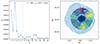 |
Fig. 2. Results of the multipole analysis of the X-ray data, in one radial aperture (ΔR)X-ray = [0.6, 1.4] Rvir. Left panel: Distribution of the multipolar ratio βm as a function of multipole order m. The limit order for the reconstruction, mmax, rec = 7, is shown as a vertical line. Right panel: Reconstructed map in the aperture (ΔR)X-ray. The white contours represent the threshold of 60% of the map maximum and identify the relevant filamentary structures, as described in the text. For reference, the X-ray hit-map is shown in the background. |
In the right panel of Fig. 2, we show the reconstructed map in the aperture (ΔR)X-ray, obtained by summing the first seven orders of the multipole decomposition shown in the left panel. In the map, we identified the relevant structures as the areas where the values are above 60% of the map maximum. These regions are delimited by white contours in the figure. We recognise three structures, which lie approximately in the north-west (NW), south (S), and east (E) directions. We see that, consistently with the expectations from the βm distribution, the NW and S structures are larger and stronger than the E structure. We also notice a mild alignment of the E and NW structures, due to the contribution of the even multipole orders (m = 2, 4).
By considering this large aperture (ΔR)X-ray = [0.6, 1.4] Rvir, we succeeded in capturing the broad distribution of structures in the outskirts of A2744. However, we lost the radial dependence information. To better recover the radial evolution, we analysed the data both inside and outside the virial radius, by splitting the aperture in two annuli: (ΔR)in = [0.6, 1.0] Rvir and (ΔR)out = [1.0, 1.4] Rvir. We show the results of the multipole decomposition in the two sub-apertures in Fig. 3.
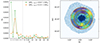 |
Fig. 3. Same as Fig. 2 but considering two radial apertures, (ΔR)in = [0.6, 1.0] Rvir (in green) and (ΔR)out = [1.0, 1.4] Rvir (in orange). |
Focusing on the inner aperture, (ΔR)in, the βm distribution is dominated by the dipole, with the octupole as second-highest peak (Fig. 3, left panel). This inversion of the dominant order (compared to the single-aperture case) suggests a strong difference between two branches of the octupole and the third, which is confirmed by the reconstructed map (right panel). There, we see that only two structures are identified: one in the south (Sin), and one in the west-northwest (NWin) direction. On the other hand, no structure is identified to the east of the aperture, where we would expect the third branch of the octupolar distribution. The reason why we cannot identify a structure in the east is that the X-ray signal in that area close to the cluster centre is weaker and extends over a larger angle, compared to the other two regions. This may be related to a shock detected in the north-east region of the cluster (Eckert et al. 2016; Hattori et al. 2017; Rajpurohit et al. 2021).
Focusing on the outer aperture, (ΔR)out, we find that βm is maximum for m = 3 (Fig. 3, left panel). All the other orders up to m = 6 are weakly contributing to the decomposition, with similar values of βm. Examining the reconstructed map of the outer aperture (Fig. 3, right panel), we can clearly identify the three structures associated with the octupolar order, in the north-west (NWout), southwest (Sout), and east (Eout) directions. We note that the NWout and Sout structures are both shifted counterclockwise with respect to their counterparts in the inner aperture, which highlights a radial dependence of these filaments across the cluster virial radius. We also see that, on top of the angular shift, NWout has a larger angular size than NWin. On the other hand the sizes of Sout and Sin are similar.
4.1.2. multipole decomposition of galaxy distribution
Due to the low statistics of the galaxy sample (305 galaxies in total, including 150 in the inner cluster region within 0.6 Rvir), we considered only one single large aperture, (ΔR)gal = [0.6, 2.1] Rvir. It contains all the 155 galaxies beyond 0.6 Rvir from the cluster centre. Figure 4 shows the βm of the galaxy distribution. The most important order of the decomposition is the octupole (m = 3), identically to the X-ray data. We can notice that the quadrupole moment (m = 2) is almost as strong as the octupole (m = 3). This suggests that there are probably three structures, with two aligned on the same axis. Indeed, the reconstructed map (Fig. 4, right panel) shows that two main structures are identified in the east and west-north-west directions (almost opposite of each other), while the third one visible in the south is less significant and does not cross our threshold of 60% of the maximum. Nonetheless, we find this southern structure to be the third strongest of the reconstructed map.
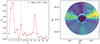 |
Fig. 4. Same as Figs. 2 and 3, but considering the 2D galaxy distribution inside one radial aperture, (ΔR)gal = [0.6, 2.1] Rvir. |
Another feature is the high peak at m = 14. This order traces very small angular scale structures. As discussed in Gouin et al. (2022), large multipole orders are correlated with the fraction of sub-structures. Indeed, by including this order into the reconstructed map, we found that it is driven by small concentrations of galaxies (about three to four galaxies with small angular separation). We notice that a similar excess of multipolar power at m = 13 − 14 is also weakly significant for X-ray data (in Figs. 2 and 3). This small-scale feature is not associated with large-scale filaments, but should rather trace sub-clumps of matter; therefore, it was not considered further in our analysis.
4.2. Filamentary structure around A2744
After analysing the angular distribution of X-ray signal and galaxy data through the multipole decomposition, we go on to focus on the filamentary structures around A2744, as detected by the filament-finding method T-REx.
4.2.1. Filaments from X-ray data
We show the result of the T-REx algorithm in Fig. 5, where we see the T-REx probability map (only values above 0.1 are shown), superimposed to the X-ray ‘hit map’. We can identify large-scale, connected, and high-probability filaments. The most prominent of them is the filament in the S-SW. From the centre to the periphery, we see it connected to the cluster in the south of the masked area, then it extends to the south-west before exhibiting a bend to the south at RA ∼ 3.5°; the last part of the structure shows reduced width and overall probability, so we do not trust it as reliable filament identification. Another structure that we can clearly identify as a filament is the NW one: connected to the cluster in the W-NW, it extends to the NW before spreading and branching out in multiple directions between north and west. Shifting our attention to the east of A2744, the identification of filaments becomes less straightforward. We can however distinguish two structures that stand out for their higher probability; both seem to depart from the same area in the E-NE of the cluster. One filament extends to the north and splits into two branches of lower reliability. The other filament extends to the east of the cluster. Finally, there are three regions where the probability is above the threshold of 0.1: west-southwest, south-east, and north-east. While we believe that these regions do not host real filaments, it might be interesting to investigate why some realisations of the T-REx algorithm identify some structures there. First of all, we should recall that this method was designed to work on much cleaner and sparser data, and that one of its main concepts is to connect over-dense regions in a coherent tree structure. This means that if, in a particular bootstrap realisation, the optimisation identifies some local overdensity in the noise, it will tend to connect it with the overall tree. However, these spurious connections will not be stable across realisations, and will not tend to accumulate into a coherent structure in the probability map. Looking at the surface brightness map, we can notice that in all three regions, there seem to be small overdensities of signal close to the cluster outside the masked region. We think that these emissions drive the algorithm to connect noise structures along those directions, thereby creating these broad, noisy probability distributions. In summary, from the analysis of the T-REx results on X-ray data we have identified four main structures as filaments extending to the south, north-west, east, and north directions.
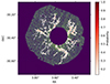 |
Fig. 5. Probability map of the filamentary structures from X-ray data, obtained with T-REx. Only pixels with probability larger than 0.1 are shown. For reference, the X-ray hit-map is shown in the background. The central part of the cluster is masked within a radius of 0.6 Rvir. |
4.2.2. Filaments from galaxy distribution
With the spectroscopic galaxies, we can access the full 3D information on the cluster and its environment. This allows the detection of structures along the LoS, which results in a more accurate estimate of the cluster connectivity. We applied T-REx to the 3D distribution of galaxies and we show the detected filamentary structures in Fig. 6.
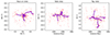 |
Fig. 6. 3D distribution of galaxies (red points) in A2744, superimposed to the 3D probability map of the filamentary structures obtained with T-REx on the galaxy data. Only voxels with probability larger than 0.1 are shown. Left: Projection along the LoS. The middle and right panels show side and top view projections, perpendicular to the LoS. |
The panels in Fig. 6 depict three projections of the galaxy distribution, with the superimposed filament probability map thresholded at 0.1 (i.e. regions where the probability is higher than 0.1). The left panel shows the projection along the LoS (with axes right ascension, RA, and declination, Dec), we call this the face-on view. The central panel has the distance along the LoS as the x axis and declination as the y axis, which we call the side view. The right panel has distance on the x axis, but the right ascension on the y axis and is referred to as the top view.
Starting from the face-on view, we can see that the T-REx algorithm identifies three filaments connected to the cluster (in the NW, E, and S directions), consistent with our previous results based on the X-ray data and with the results of Eckert et al. (2015). We notice how the S filament is considerably shorter than the other two; this is in line with the results of the multipole analysis, where we found that in the south region the over-density of galaxies is less significant than in the other zones. Another noticeable feature is the rather sharp bend in the NW filament at RA ∼ 3.4°, connecting a concentration of galaxies in the far west of the field. This is probably due to a selection effect, given it is so close to the edge of the observations.
Moving to the side view, we observe the cluster and its surrounding structures along the LoS (on the x axis). The first thing we notice is the presence of an elongated structure in the radial direction, which extends both in front and behind the centre of the galaxy distribution, at relatively the same declination. We call this the central structure. Moreover, we observe that T-REx identifies a structure at the rear of the cluster, slightly separated from the main branch in the LoS, which corresponds to the southern concentration of galaxies in the face-on view (at roughly RA ∼ 3.6°, Dec ∼ −30.4°). We can also see again the southern filament from a different point of view, and we see that it has very little extension in the LoS direction, and that it connects to the central structure a little in front of the centre of the galaxy distribution.
Finally, from the top view, we can extract some interesting information about the E and NW filaments. In fact, we see that the E filament connects to the central structure in approximately the same position as the S filament. On the other hand, the NW filament is connected further back, in a location that we can associate approximately with an X-ray peak in the north-west of the cluster centre. Moreover, we observe that both these filaments (actually all three, considering also the S one) do not extend much in the radial direction, and tend to be roughly perpendicular to the LoS. Lastly, we see that the central structure is not exactly parallel to the LoS, but tends to extend from east to west as the distance increases, with the exception of the front-most part.
Putting everything together, we draw a picture of the 3D structure of the A2744 cluster surroundings. We detect three filaments almost perpendicular to the LoS; a long, extended filamentary structure along the LoS and a disconnected structure at the back of the cluster (slightly south-east of the centre). Two of the filaments (E and S) connect in the same position in the front-eastern part of the cluster, while the NW filament is connected in the back of the cluster, towards the west. Along the LoS, the central structure extends beyond the virial radius both in front and behind the cluster: the front branch is located roughly at the centre of the cluster on the plane of the sky, almost parallel to the LoS; in the back of the cluster, the branch extends towards the west from the connecting point of the NW filament. Also, in the back of the cluster, T-REx identifies another structure not directly connected to the main one, but crossing the virial sphere of the cluster. Located in the southwest of the cluster centre, this back structure can be associated with the southern peak in the X-ray surface brightness map.
Comparing the probability map obtained from the X-ray data with that from the 3D galaxy distribution (Fig. 7), we note some important differences. The first one is clearly the impossibility of reconstructing from the X-ray data the two filamentary structures along the LoS, identified in the galaxy distribution. On the plane of the sky, we note the lack of a counterpart in the galaxy data for the X-ray-detected N structure. This confirms the results of Eckert et al. (2015), which also identified a northern structure in the X-ray map, but discarded it due to the lack of galaxies in the region (the X-ray emission was associated instead with a background galaxy concentration). Another interesting difference is the length of the southern filament. In Fig. 5, we see it extends to a considerable length in the SW region, while in the galaxy case, only the part close to the cluster is traced, out to ∼1 Rvir. A possible explanation for this difference is a lack of galaxies in the southwestern region due to the lower completeness estimated by Owers et al. (2011) (Fig. 9). The non-uniform spectroscopic completeness might also explain the different shape of the NW filament in the two T-REx probability maps, since the western region around Rvir is also reported to have a lower level of completeness in the study by Owers et al. (2011).
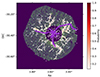 |
Fig. 7. Comparison of the T-REx probability map from X-ray data (Fig. 5) and the face-on projection of the T-REx probability map from galaxy data (Fig. 6, left panel). For reference, both the X-ray hit-map and the galaxy distribution are shown in the background. |
5. Robustness of results
To assess the robustness of the results presented in Sect. 4, we performed several tests, exploring different choices both in the data pre-processing and the parameters of the methods used.
5.1. Robustness to data preprocessing choices
We tested the impact of some of the choices described in Sect. 2. For the baseline analysis of the X-ray data, we used a conservative point-source mask (see Sect. 2.1 for details). We tested the impact of this choice by repeating both the multipole analysis and the T-REx filament detection, masking only the high-reliability point sources (i.e. those obtained by cross-matching the point sources lists detected in the soft and hard energy bands). The results obtained from this set-up (Fig. 8) are very similar to those of the baseline set-up (Figs. 2 and 5). We can notice some small differences in the βm distribution (Fig. 8, left panel), but the reconstructed map (middle panel) does not change appreciably. The T-REx probability map (Fig. 8, right panel) highlights the same four filaments as with the conservative point-source mask and it looks somewhat less noisy. This is probably due to the alignment of some compact emissions with the filament signal, which helps the T-REx algorithm orient in those directions.
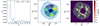 |
Fig. 8. Results of the multipole decomposition and T-REx analyses, using the X-ray data with just the high-reliability point sources masked (see text). Left and middle: Multipole analysis, same as Fig. 2. Right: T-REx probability map, same as Fig. 5. |
Moving on to the 3D galaxy distribution, one assumption in the baseline analysis is the magnitude cut at rF < 20.5, based on the spectroscopic completeness. We explored the impact of this choice. In practice, we relaxed this constraint to rF < 21, corresponding to 412 galaxies (35% more than the baseline) and repeated the analysis. Again, the results are consistent with the baseline analysis. The reconstructed map from the multipole decomposition shows the same two main structures (E and NW) as the baseline analysis, while the southern one is also found below the threshold. The T-REx probability map is more complex than in the baseline analysis due to the larger number of galaxies, especially in the central region of A2744.
5.2. Robustness to method parameters
We also tested the robustness of the analysis techniques, particularly with respect to the choice of their free parameters. For the multipole analysis, we focused on the impact of the size of the aperture (i.e. the choice of the radial boundaries of the annulus). The choice of the aperture boundaries, Rmin and Rmax, clearly influences the results. This is shown, for example, in Fig. 3, where we compare two subsequent apertures. Nonetheless, we find that for the X-ray data in the single aperture case the qualitative results are quite stable across a large range of radial limits. For example, if we fix Rmax at 1.4 Rvir and vary Rmin from 0 to 1.2 Rvir, we find that the most important order is always the octupole; meanwhile the relative powers of the other orders vary, but the structures identified in the reconstructed map are always three, with small differences in position. On the other hand, when fixing Rmin to 0.6 Rvir and varying Rmax, we find that between 0.8 and 1.3 Rvir the dipole dominates over the octupole in the βm distribution and in the reconstructed maps, only the S and NW structures can be identified clearly (as is the case for the inner aperture in Fig. 3). After this radius, the octupolar order becomes dominant and we find back the three filaments of the main analysis, mostly unchanged up to Rmax = 1.5 Rvir, which is the maximum distance we can reach before hitting the western border of the field.
The analysis of the galaxy data is significantly different in this respect. When dealing with a small number of galaxies, the multipole decomposition becomes particularly noisy, and the inclusion or exclusion of just a few galaxies significantly changes the results. Therefore, we need to use a large enough aperture to accumulate statistics. In the baseline analysis, we made the conservative choice of including all galaxies located beyond 0.6 Rvir from the cluster’s centre. Fixing Rmin = 0.6 Rvir and progressively increasing the aperture size ΔR, we can first identify two structures in the south and north-west directions (up to Rmax ∼ 1.5 Rvir), then the southern one disappears; later, the eastern structure appears (around 1.7 Rvir) and becomes more prominent as we expand the aperture to larger radii.
Regarding the T-REx algorithm, we conducted several tests to minimise the noise of the probability maps and ensure the best convergence of the trees. There are two main parameters we tested: the denoising parameter, l, and the strength of the tree prior, λ (described in detail in Bonnaire et al. 2020). The first parameter acts on the initial MST, on which an iterative pruning of all end-point branches is repeated l times, denoising the tree while retaining the relevant long branches. The second parameter, λ, regulates the strength of the topological constraint in the optimisation, which tends to reduce the overall length of the graph. Higher values of λ thus produce smoother and simpler filamentary structures (generally avoiding overfitting), but also tend to produce shorter branches, often at the expense of data fidelity.
T-REx has already been applied successfully on simulations to trace the cosmic web by Bonnaire et al. (2020), Gouin et al. (2021) and on 2D and 3D galaxy distributions in Aghanim et al. (2024). Therefore, in the present work, for the galaxy case we only slightly adapted the parameters, notably reducing the denoising parameter l to account for the lower number of galaxies. For the case of the X-ray data, instead, we needed to adapt the parameters to the very different regime, with a large number of points and high noise level, as discussed in Sect. 4.2. We found that a combination of high denoising l and high λ helps in reducing the noise in the probability map. In our tests, iteratively pruning the tree a large number of times proved useful in removing spurious detection. Looking at the onion decomposition (Hébert-Dufresne et al. 2016 as suggested by Bonnaire et al. 2020), we found that choosing l ∼ 200 still allows for a large number of nodes to survive, thus allowing the tree to trace well peripheral areas. The choice of λ is dictated by the need to reduce overfitting in the presence of a very large number of nodes, as explained in Bonnaire et al. (2022).
Qualitatively, we find that the results of T-REx are consistent for a large range of the parameters’ values and that the regions we identified as filaments tend to have higher probabilities even in very noisy realisations of the probability map. This reduces the need to find optimal free parameters.
6. Discussion
The outskirts of the cluster of galaxies A2744 have been the target of different studies, which probed them with spectroscopic galaxy and X-rays observations (Braglia et al. 2007; Owers et al. 2011; Ibaraki et al. 2014; Eckert et al. 2015; Hattori et al. 2017). Braglia et al. (2007) used a sample of 194 spectroscopic galaxies observed with the VIsible MultiObject Spectrograph at ESO’s Very Large Telescope (VLT-VIMOS). Owers et al. (2011) used the same sample of galaxies we used in this work. Both studies combined position and velocity information, finding two overdense regions in the south and north-west of A2744, which were identified as large-scale filaments. Owers et al. (2011) also highlighted an overdensity of galaxies in the east of the cluster, but found that the local velocity distribution does not differ significantly from the overall cluster distribution, so it was not identified as a relevant structure by the authors.
Eckert et al. (2015) identified six regions of extended emission connected to the cluster from the adaptively smoothed X-ray surface brightness map (in the soft energy band). Four of these filamentary structures were found to coincide with galaxy concentrations: one in the north-west (NWE15), two in the south and southwest (S+SWE15), and one in the east (EE15). The first two regions correspond to the findings of Braglia et al. (2007) and Owers et al. (2011), the east one to the overdensity of Owers et al. (2011). The other two X-ray emission regions (in the south-east, SEE15, and north, NE15) were associated with concentrations of galaxies not connected to A2744. Analysing the X-ray spectra in the detected regions, Eckert et al. (2015) and Hattori et al. (2017) found evidence that the gas originating the X-ray emission is in the form of warm-hot intergalactic medium (WHIM). This supports the identification of these regions as cosmic filaments, since several studies have shown that in hydrodynamical simulations, the WHIM is the most important gas phase in cosmic filaments and can be reliably used to trace them (Martizzi et al. 2019; Galárraga-Espinosa et al. 2021; Tuominen et al. 2021; Gouin et al. 2022). Furthermore (and again from simulations), Gouin et al. (2023) showed that the dominant source of soft X-rays beyond the virial radius is the warm gas in the WHIM and warm circumgalactic medium (WCGM), instead of the hot gas of the intra-cluster medium (ICM) that dominates inside Rvir.
In this work, we performed the first blind detection of filaments around A2744, using a filament-finder technique and reconstructed maps from a multipole decomposition technique, applied both to the X-ray data and to the galaxy distribution.
In Fig. 9, we compare the structures identified with our two methods, for X-ray (left panel) and galaxy (right panel) data, with the X-ray-identified structures (white ellipses) from Eckert et al. (2015) (and thus, implicitly, with the other works mentioned above). From the X-ray data, we see that for the NW, S, and E structures, there is a very close correspondence between the results of our two methods. The detected filaments from T-REx match the region identified in the reconstructed maps well, both in terms of position and radial dependence, including the gap between the cluster and the E filament. These structures are also well in agreement with the NWE15, (S+SW)E15, and EE15 regions from Eckert et al. (2015). The fact that these regions (the ones with confirmed galaxy counterparts in Eckert et al. 2015) are the ones where our methods agree highlights the complementarity of the two methods, and the robustness of their combined detections. We also note that the N filament, detected by T-REx, has no significant match in the multipole analysis, but it does match with a structure (NE15) first identified and then discarded by Eckert et al. (2015). Finally, the SEE15 ellipse has no detected counterpart in either of our two methods.
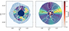 |
Fig. 9. Results of the multipole and T-REx analyses, on X-ray data (left) and on galaxy data (right). The reconstructed map from the multipole decomposition is superimposed on the T-REx probability map. The white ellipses correspond to the regions identified in Eckert et al. (2015). For reference, the X-ray hit-map is shown in the background. |
For the galaxy data, we recall that the T-REx algorithm is run on the 3D distribution of galaxies, while the multipole analysis is done on the projected 2D distribution. Comparing the results of the two methods along the LoS (Fig. 9, right panel), we see that in the east, the T-REx-detected filament overlaps well with the E structure in the reconstructed map and with the EE15 ellipse. In the north-west, the overlap between the different detections is only partial, but they all agree on the presence of a structure in this area. The reasons for these differences might be selection effects (due to the non-spatially-uniform completeness of the galaxy sample) or border effects. In the south, as we mentioned in Sects. 4.1.2 and 4.2.2, the detection of a filamentary structure is more difficult: the T-REx algorithm detects a filament, but it only extends to ∼Rvir, while in the same region the reconstructed map has its third-highest structure, but this does not meet the detection threshold. This might be again due to lower completeness in the area (see Owers et al. 2011, Fig. 9).
Combining our results from X-ray and galaxy data, we can draw a comprehensive picture of the surroundings of the cluster A2744. From our analysis of A2744 on the plane of the sky, we identified three filaments connected to the cluster (NW, S, and E). These three are consistent across almost all the combinations of probe (X-rays or galaxies) and detection method (T-REx or azimuthal analysis), with a larger uncertainty for the S filament in galaxy data, which is also consistent with previous works. All three extend out to ∼1.5 Rvir, thus yielding a 2D connectivity of κ2D = 3. In addition, analysing the 3D galaxy distribution with T-REx, we identified two filamentary structures along the LoS: one in the front and one in the back of the cluster. The exact extent of these structures may however depend on the specific FoG correction we applied to the galaxy sample. In total, we identified five filamentary structures connected to the core of A2744 in three dimensions (κ3D = 5).
This wealth of connected structures can help explain the particularly complex internal structure of the cluster. A2744 is known for its exceptional number of massive sub-structures, which make it a very dynamically disturbed cluster (Merten et al. 2011; Owers et al. 2011; Jauzac et al. 2015, 2016; Medezinski et al. 2016; Bergamini et al. 2023; Harvey & Massey 2024). Cosmic filaments act as highways, along which gas and dark matter preferentially fall into clusters (Rost et al. 2021). Thus, they can point to the origin and direction of some sub-structures. For example, Jauzac et al. (2016) reported the alignment of three sub-structures in the direction of the NW filament. Another sub-structure in the north of the central cluster area shows evidence of a northward movement (Owers et al. 2011; Jauzac et al. 2016), suggesting a possible origin in the direction of the S filament. In a similar way, a shock front detected in the south-east of the cluster centre (Owers et al. 2011) suggests the motion of sub-structures coming from the north-west.
Broadening the view, we compare our results with those on larger cluster populations. It has been shown from both simulations and observations (Aragón-Calvo et al. 2010; Codis et al. 2018; Darragh Ford et al. 2019; Sarron et al. 2019; Kraljic et al. 2020; Lee et al. 2021; Gouin et al. 2021; Galárraga-Espinosa et al. 2024; Santoni et al. 2024) that higher mass clusters tend to have higher connectivity. Moreover, Gouin et al. (2021) showed that, for the same mass, dynamically unrelaxed clusters are generally more connected than relaxed ones. A value of κ3D = 5 for the connectivity of A2744 is therefore in agreement with trends from hydrodynamical simulations. Comparing to other observations of individual clusters, the connectivity of the Coma cluster (M200 = 5.3 × 10¹⁴ M⊙, Gavazzi et al. 2009) has been determined to be κ = 3 (Malavasi et al. 2020, 2023), which seems to be in line with the connectivity of simulated relaxed clusters (Gouin et al. 2021). On the other hand, Einasto et al. (2020, 2021) studied the connectivity of clusters in superclusters. In these dense environments, massive clusters were found to be highly connected. For example, A2142 (M200 = 1.2 × 10¹⁵ M⊙, Munari et al. 2014) exhibits κ = 6 − 7 (Einasto et al. 2020) and A2065 (M200 = 2.3 × 10¹⁵ M⊙, Pearson et al. 2014) is even more connected, with κ = 9.
7. Conclusions
In this work, we present an analysis of the X-ray and galaxy distributions surrounding the galaxy cluster A2744, along with the identification of filamentary structures connected to the cluster. This was done using two methods: the aperture multipole decomposition, which highlights the azimuthal structure of the considered field in a given annulus, and the filament-finding method T-REx, which extracts the ridges in a discrete distribution using a statistical tree-based description. While both techniques are efficient at identifying filamentary structures in two dimensions (as is the case for the X-ray data), only T-REx is able to do that in three dimensions, leveraging the full information of the spectroscopic galaxy sample. Therefore, we were able to probe the structures along the LoS only with T-REx. We present a brief summary of our results below.
-
We report, for the first time, the blind detection of filaments connected to a cluster from X-ray data. Both methods we applied showed three clear filamentary structures in the south (S), north-west (NW), and east (E) of the cluster. These are consistent with a prior visual detection by Eckert et al. (2015).
-
All three filaments were extracted from the distribution of galaxies at approximately the same (projected) positions as their X-ray counterparts, although the south filament was detected only by the T-REx method.
-
The X-ray-based T-REx probability map showed an additional structure in the north, coincident to one identified by Eckert et al. (2015), but it was not confirmed by the multipole analysis, nor supported by the galaxy data.
-
Through the galaxy distribution, we studied the 3D filamentary structure extracted with the T-REx method: we found that the three filaments detected in 2D are all almost perpendicular to the LoS. The south and east filaments lie almost on the same plane, while the north-west one is found further in the back and connects to a different part of the cluster. The central part of the cluster is strongly elongated in the radial direction and extends beyond Rvir, both in the front and back. Furthermore, a loosely connected structure is identified in the back of the cluster, which seems to be aligned with the southern X-ray peak.
-
The number and positions of the detected filaments can improve the interpretation of the highly disturbed cluster centre, particularly concerning the origin and direction of motion of its many sub-structures.
-
We estimated the 3D connectivity of A2744 to be κ3D = 5, which is in agreement with trends from hydrodynamical simulations for a massive, disturbed cluster.
Thanks to the combination of different methods for identifying filamentary structures, applied to different probes, we were able to confirm the possibility of the blind detection of filaments in the outskirts of galaxy clusters. This result could open the way to a systematic search for cosmic filaments connected to clusters, particularly with respect to the gas component and in the context of large X-ray programs such as eROSITA (Bulbul et al. 2024), CHEX-MATE (CHEX-MATE Collaboration 2021), and XRISM (XRISM Science Team 2020).
Acknowledgments
The authors thank the anonymous referee for their constructive comments. The authors thank S. Ettori for discussions during the initial stage of the project. This work was supported by funding from the ByoPiC project from the European Research Council (ERC) under the European Union’s Horizon 2020 research and innovation program grant number ERC-2015-AdG 695561. SG acknowledges financial support from the Ecole Doctorale d’Astronomie et d’Astrophysique d’Ile-de-France (ED AAIF). CG acknowledges funding from the French Agence Nationale de la Recherche for the project WEAVEQSO-JPAS (ANR-22-CE31-0026).
References
- Aghanim, N., Tuominen, T., Bonjean, V., et al. 2024, A&A, 689, A332 [NASA ADS] [CrossRef] [EDP Sciences] [Google Scholar]
- Aragón-Calvo, M. A., van de Weygaert, R., & Jones, B. J. T. 2010, MNRAS, 408, 2163 [CrossRef] [Google Scholar]
- Bergamini, P., Acebron, A., Grillo, C., et al. 2023, ApJ, 952, 84 [NASA ADS] [CrossRef] [Google Scholar]
- Bond, J. R., Kofman, L., & Pogosyan, D. 1996, Nature, 380, 603 [NASA ADS] [CrossRef] [Google Scholar]
- Bonjean, V., Aghanim, N., Salomé, P., Douspis, M., & Beelen, A. 2018, A&A, 609, A49 [NASA ADS] [CrossRef] [EDP Sciences] [Google Scholar]
- Bonnaire, T., Aghanim, N., Decelle, A., & Douspis, M. 2020, A&A, 637, A18 [NASA ADS] [CrossRef] [EDP Sciences] [Google Scholar]
- Bonnaire, T., Decelle, A., & Aghanim, N. 2022, IEEE Trans. Pattern Anal. Mach. Intell., 44, 9119 [CrossRef] [Google Scholar]
- Boschin, W., Girardi, M., Spolaor, M., & Barrena, R. 2006, A&A, 449, 461 [NASA ADS] [CrossRef] [EDP Sciences] [Google Scholar]
- Braglia, F., Pierini, D., & Böhringer, H. 2007, A&A, 470, 425 [NASA ADS] [CrossRef] [EDP Sciences] [Google Scholar]
- Braglia, F. G., Pierini, D., Biviano, A., & Böhringer, H. 2009, A&A, 500, 947 [NASA ADS] [CrossRef] [EDP Sciences] [Google Scholar]
- Bulbul, E., Randall, S. W., Bayliss, M., et al. 2016, ApJ, 818, 131 [Google Scholar]
- Bulbul, E., Liu, A., Kluge, M., et al. 2024, A&A, 685, A106 [NASA ADS] [CrossRef] [EDP Sciences] [Google Scholar]
- Buote, D. A., & Tsai, J. C. 1995, ApJ, 452, 522 [Google Scholar]
- Campitiello, M. G., Ettori, S., Lovisari, L., et al. 2022, A&A, 665, A117 [NASA ADS] [CrossRef] [EDP Sciences] [Google Scholar]
- CHEX-MATE Collaboration (Arnaud, M., et al.) 2021, A&A, 650, A104 [NASA ADS] [CrossRef] [EDP Sciences] [Google Scholar]
- Codis, S., Pogosyan, D., & Pichon, C. 2018, MNRAS, 479, 973 [Google Scholar]
- Couch, W. J., & Sharples, R. M. 1987, MNRAS, 229, 423 [NASA ADS] [CrossRef] [Google Scholar]
- Couch, W. J., Barger, A. J., Smail, I., Ellis, R. S., & Sharples, R. M. 1998, ApJ, 497, 188 [NASA ADS] [CrossRef] [Google Scholar]
- Darragh Ford, E., Laigle, C., Gozaliasl, G., et al. 2019, MNRAS, 489, 5695 [Google Scholar]
- de Graaff, A., Cai, Y.-C., Heymans, C., & Peacock, J. A. 2019, A&A, 624, A48 [NASA ADS] [CrossRef] [EDP Sciences] [Google Scholar]
- De Luca, F., De Petris, M., Yepes, G., et al. 2021, MNRAS, 504, 5383 [NASA ADS] [CrossRef] [Google Scholar]
- Dietrich, J. P., Schneider, P., Clowe, D., Romano-Díaz, E., & Kerp, J. 2005, A&A, 440, 453 [NASA ADS] [CrossRef] [EDP Sciences] [Google Scholar]
- Eckert, D., Jauzac, M., Shan, H., et al. 2015, Nature, 528, 105 [Google Scholar]
- Eckert, D., Jauzac, M., Vazza, F., et al. 2016, MNRAS, 461, 1302 [Google Scholar]
- Eckert, D., Finoguenov, A., Ghirardini, V., et al. 2020, Open J. Astrophys., 3, 12 [NASA ADS] [CrossRef] [Google Scholar]
- Einasto, M., Deshev, B., Tenjes, P., et al. 2020, A&A, 641, A172 [NASA ADS] [CrossRef] [EDP Sciences] [Google Scholar]
- Einasto, M., Kipper, R., Tenjes, P., et al. 2021, A&A, 649, A51 [NASA ADS] [CrossRef] [EDP Sciences] [Google Scholar]
- Galárraga-Espinosa, D., Aghanim, N., Langer, M., & Tanimura, H. 2021, A&A, 649, A117 [Google Scholar]
- Galárraga-Espinosa, D., Cadiou, C., Gouin, C., et al. 2024, A&A, 684, A63 [NASA ADS] [CrossRef] [EDP Sciences] [Google Scholar]
- Gavazzi, R., Adami, C., Durret, F., et al. 2009, A&A, 498, L33 [NASA ADS] [CrossRef] [EDP Sciences] [Google Scholar]
- Ghirardini, V., Eckert, D., Ettori, S., et al. 2019, A&A, 621, A41 [NASA ADS] [CrossRef] [EDP Sciences] [Google Scholar]
- Gouin, C., Gavazzi, R., Codis, S., et al. 2017, A&A, 605, A27 [NASA ADS] [CrossRef] [EDP Sciences] [Google Scholar]
- Gouin, C., Aghanim, N., Bonjean, V., & Douspis, M. 2020, A&A, 635, A195 [NASA ADS] [CrossRef] [EDP Sciences] [Google Scholar]
- Gouin, C., Bonnaire, T., & Aghanim, N. 2021, A&A, 651, A56 [NASA ADS] [CrossRef] [EDP Sciences] [Google Scholar]
- Gouin, C., Gallo, S., & Aghanim, N. 2022, A&A, 664, A198 [NASA ADS] [CrossRef] [EDP Sciences] [Google Scholar]
- Gouin, C., Bonamente, M., Galárraga-Espinosa, D., Walker, S., & Mirakhor, M. 2023, A&A, 680, A94 [NASA ADS] [CrossRef] [EDP Sciences] [Google Scholar]
- Govoni, F., Enßlin, T. A., Feretti, L., & Giovannini, G. 2001, A&A, 369, 441 [NASA ADS] [CrossRef] [EDP Sciences] [Google Scholar]
- Harvey, D. R., & Massey, R. 2024, MNRAS, 529, 802 [NASA ADS] [CrossRef] [Google Scholar]
- Hattori, S., Ota, N., Zhang, Y.-Y., Akamatsu, H., & Finoguenov, A. 2017, PASJ, 69, 39 [CrossRef] [Google Scholar]
- Hébert-Dufresne, L., Grochow, J. A., & Allard, A. 2016, Sci. Rep., 6, 31708 [CrossRef] [Google Scholar]
- Hwang, H. S., Geller, M. J., Park, C., et al. 2016, ApJ, 818, 173 [NASA ADS] [CrossRef] [Google Scholar]
- Ibaraki, Y., Ota, N., Akamatsu, H., Zhang, Y. Y., & Finoguenov, A. 2014, A&A, 562, A11 [NASA ADS] [CrossRef] [EDP Sciences] [Google Scholar]
- Ilc, S., Fabjan, D., Rasia, E., Borgani, S., & Dolag, K. 2024, A&A, 690, A32 [NASA ADS] [CrossRef] [EDP Sciences] [Google Scholar]
- Jackson, J. C. 1972, MNRAS, 156, 1P [CrossRef] [Google Scholar]
- Jauzac, M., Richard, J., Jullo, E., et al. 2015, MNRAS, 452, 1437 [Google Scholar]
- Jauzac, M., Eckert, D., Schwinn, J., et al. 2016, MNRAS, 463, 3876 [NASA ADS] [CrossRef] [Google Scholar]
- Kempner, J. C., & David, L. P. 2004, MNRAS, 349, 385 [NASA ADS] [CrossRef] [Google Scholar]
- Kraljic, K., Pichon, C., Codis, S., et al. 2020, MNRAS, 491, 4294 [Google Scholar]
- Kuchner, U., Aragón-Salamanca, A., Pearce, F. R., et al. 2020, MNRAS, 494, 5473 [NASA ADS] [CrossRef] [Google Scholar]
- Lee, J., Shin, J., Snaith, O. N., et al. 2021, ApJ, 908, 11 [CrossRef] [Google Scholar]
- Limousin, M., Morandi, A., Sereno, M., et al. 2013, Space Sci. Rev., 177, 155 [Google Scholar]
- Malavasi, N., Aghanim, N., Tanimura, H., Bonjean, V., & Douspis, M. 2020, A&A, 634, A30 [NASA ADS] [CrossRef] [EDP Sciences] [Google Scholar]
- Malavasi, N., Sorce, J. G., Dolag, K., & Aghanim, N. 2023, A&A, 675, A76 [NASA ADS] [CrossRef] [EDP Sciences] [Google Scholar]
- Martizzi, D., Vogelsberger, M., Artale, M. C., et al. 2019, MNRAS, 486, 3766 [Google Scholar]
- Mead, J. M. G., King, L. J., & McCarthy, I. G. 2010, MNRAS, 401, 2257 [CrossRef] [Google Scholar]
- Medezinski, E., Umetsu, K., Okabe, N., et al. 2016, ApJ, 817, 24 [NASA ADS] [CrossRef] [Google Scholar]
- Merten, J., Coe, D., Dupke, R., et al. 2011, MNRAS, 417, 333 [NASA ADS] [CrossRef] [Google Scholar]
- Munari, E., Biviano, A., & Mamon, G. A. 2014, A&A, 566, A68 [NASA ADS] [CrossRef] [EDP Sciences] [Google Scholar]
- Owers, M. S., Randall, S. W., Nulsen, P. E. J., et al. 2011, ApJ, 728, 27 [Google Scholar]
- Pearson, D. W., Batiste, M., & Batuski, D. J. 2014, MNRAS, 441, 1601 [Google Scholar]
- Planck Collaboration VI. 2020, A&A, 641, A6 [NASA ADS] [CrossRef] [EDP Sciences] [Google Scholar]
- Planck Collaboration Int. VIII. 2013, A&A, 550, A134 [NASA ADS] [CrossRef] [EDP Sciences] [Google Scholar]
- Rajpurohit, K., Vazza, F., van Weeren, R. J., et al. 2021, A&A, 654, A41 [NASA ADS] [CrossRef] [EDP Sciences] [Google Scholar]
- Rasia, E., Meneghetti, M., & Ettori, S. 2013, Astron. Rev., 8, 40 [Google Scholar]
- Reiprich, T. H., Basu, K., Ettori, S., et al. 2013, Space Sci. Rev., 177, 195 [Google Scholar]
- Rost, A., Kuchner, U., Welker, C., et al. 2021, MNRAS, 502, 714 [Google Scholar]
- Santoni, S., De Petris, M., Yepes, G., et al. 2024, A&A, 692, A44 [NASA ADS] [CrossRef] [EDP Sciences] [Google Scholar]
- Sarron, F., Adami, C., Durret, F., & Laigle, C. 2019, A&A, 632, A49 [NASA ADS] [CrossRef] [EDP Sciences] [Google Scholar]
- Schneider, P., & Bartelmann, M. 1997, MNRAS, 286, 696 [Google Scholar]
- Shin, T.-H., Clampitt, J., Jain, B., et al. 2018, MNRAS, 475, 2421 [Google Scholar]
- Tanimura, H., Hinshaw, G., McCarthy, I. G., et al. 2019, MNRAS, 483, 223 [Google Scholar]
- Tanimura, H., Aghanim, N., Kolodzig, A., Douspis, M., & Malavasi, N. 2020, A&A, 643, L2 [EDP Sciences] [Google Scholar]
- Tanimura, H., Aghanim, N., Douspis, M., & Malavasi, N. 2022, A&A, 667, A161 [NASA ADS] [CrossRef] [EDP Sciences] [Google Scholar]
- Tegmark, M., Blanton, M. R., Strauss, M. A., et al. 2004, ApJ, 606, 702 [Google Scholar]
- Tempel, E., Tago, E., & Liivamägi, L. J. 2012, A&A, 540, A106 [CrossRef] [EDP Sciences] [Google Scholar]
- Tuominen, T., Nevalainen, J., Tempel, E., et al. 2021, A&A, 646, A156 [EDP Sciences] [Google Scholar]
- Veronica, A., Reiprich, T. H., Pacaud, F., et al. 2024, A&A, 681, A108 [NASA ADS] [CrossRef] [EDP Sciences] [Google Scholar]
- Walker, S., & Lau, E. 2022, Handbook of X-ray and Gamma-ray Astrophysics, 13 [Google Scholar]
- Walker, S., Simionescu, A., Nagai, D., et al. 2019, Space Sci. Rev., 215, 7 [Google Scholar]
- Werner, N., Finoguenov, A., Kaastra, J. S., et al. 2008, A&A, 482, L29 [NASA ADS] [CrossRef] [EDP Sciences] [Google Scholar]
- XRISM Science Team 2020, ArXiv e-prints [arXiv:2003.04962] [Google Scholar]
- Zakharova, D., Vulcani, B., De Lucia, G., et al. 2023, MNRAS, 525, 4079 [NASA ADS] [CrossRef] [Google Scholar]
All Figures
|
Fig. 1. Illustration of the different angular symmetries associated to the different multipole orders, m. |
| In the text | |
|
Fig. 2. Results of the multipole analysis of the X-ray data, in one radial aperture (ΔR)X-ray = [0.6, 1.4] Rvir. Left panel: Distribution of the multipolar ratio βm as a function of multipole order m. The limit order for the reconstruction, mmax, rec = 7, is shown as a vertical line. Right panel: Reconstructed map in the aperture (ΔR)X-ray. The white contours represent the threshold of 60% of the map maximum and identify the relevant filamentary structures, as described in the text. For reference, the X-ray hit-map is shown in the background. |
| In the text | |
|
Fig. 3. Same as Fig. 2 but considering two radial apertures, (ΔR)in = [0.6, 1.0] Rvir (in green) and (ΔR)out = [1.0, 1.4] Rvir (in orange). |
| In the text | |
|
Fig. 4. Same as Figs. 2 and 3, but considering the 2D galaxy distribution inside one radial aperture, (ΔR)gal = [0.6, 2.1] Rvir. |
| In the text | |
|
Fig. 5. Probability map of the filamentary structures from X-ray data, obtained with T-REx. Only pixels with probability larger than 0.1 are shown. For reference, the X-ray hit-map is shown in the background. The central part of the cluster is masked within a radius of 0.6 Rvir. |
| In the text | |
|
Fig. 6. 3D distribution of galaxies (red points) in A2744, superimposed to the 3D probability map of the filamentary structures obtained with T-REx on the galaxy data. Only voxels with probability larger than 0.1 are shown. Left: Projection along the LoS. The middle and right panels show side and top view projections, perpendicular to the LoS. |
| In the text | |
|
Fig. 7. Comparison of the T-REx probability map from X-ray data (Fig. 5) and the face-on projection of the T-REx probability map from galaxy data (Fig. 6, left panel). For reference, both the X-ray hit-map and the galaxy distribution are shown in the background. |
| In the text | |
|
Fig. 8. Results of the multipole decomposition and T-REx analyses, using the X-ray data with just the high-reliability point sources masked (see text). Left and middle: Multipole analysis, same as Fig. 2. Right: T-REx probability map, same as Fig. 5. |
| In the text | |
|
Fig. 9. Results of the multipole and T-REx analyses, on X-ray data (left) and on galaxy data (right). The reconstructed map from the multipole decomposition is superimposed on the T-REx probability map. The white ellipses correspond to the regions identified in Eckert et al. (2015). For reference, the X-ray hit-map is shown in the background. |
| In the text | |
Current usage metrics show cumulative count of Article Views (full-text article views including HTML views, PDF and ePub downloads, according to the available data) and Abstracts Views on Vision4Press platform.
Data correspond to usage on the plateform after 2015. The current usage metrics is available 48-96 hours after online publication and is updated daily on week days.
Initial download of the metrics may take a while.