| Issue |
A&A
Volume 692, December 2024
|
|
|---|---|---|
| Article Number | A116 | |
| Number of page(s) | 8 | |
| Section | The Sun and the Heliosphere | |
| DOI | https://doi.org/10.1051/0004-6361/202449558 | |
| Published online | 05 December 2024 | |
Turbulent plasma flow, its energies, and structures: Velocity vortices, magnetic field cocoons, and plasmoids
1
University of South Bohemia, Faculty of Science, Department of Physics, Branišovská 1760, CZ – 370 05 České Budějovice, Czech Republic
2
Astronomical Institute of the Czech Academy of Sciences, Fričova 258, CZ – 251 65 Ondřejov, Czech Republic
⋆ Corresponding author; This email address is being protected from spambots. You need JavaScript enabled to view it.
Received:
9
February
2024
Accepted:
27
October
2024
Abstract
Context. Turbulent flows are believed to be present in the solar corona, especially in connection with solar flares and coronal mass ejections. They are supposed to be very effective processes in energy transportation and can contribute to the heating of the solar corona.
Aims. We study turbulence in reconnection outflows associated with flares and coronal mass ejections. We simulated the generation and evolution of the turbulent plasma flow and investigated its energies and formed plasma velocity and magnetic field structures.
Methods. For the numerical simulations, we adopted a three-dimensional (3D) magnetohydrodynamic (MHD) model, in which we solved a full set of the 3D time-dependent resistive and compressible MHD equations using the LARE3D numerical code.
Results. We numerically studied turbulence in the plasma flow in the model with the plasma parameters that could simulate processes in the magnetic reconnection outflows in solar flares. Starting from a non-turbulent plasma flow in the energetically closed system, we studied the evolution of the kinetic, internal, and magnetic energies during the turbulence generation. We found that most of the kinetic energy is transformed into the plasma heating (about 95%) and only a small part to the magnetic energy (about 5%). The turbulence in the system evolves to the saturation stage with the power-law index of the kinetic density spectrum, −5/3. Magnetic energy is also saturated due to its dissipation and reconnection in small and complex magnetic field structures. We show examples of the structures formed in studied turbulent flow: velocity vortices, magnetic field cocoons, and plasmoids.
Key words: magnetohydrodynamics (MHD) / turbulence / methods: numerical / Sun: corona / Sun: coronal mass ejections (CMEs) / Sun: flares
© The Authors 2024
 Open Access article, published by EDP Sciences, under the terms of the Creative Commons Attribution License (https://creativecommons.org/licenses/by/4.0), which permits unrestricted use, distribution, and reproduction in any medium, provided the original work is properly cited.
This article is published in open access under the Subscribe to Open model. This email address is being protected from spambots. You need JavaScript enabled to view it. to support open access publication.
1. Introduction
Turbulence and magnetic field reconnection are closely associated with each other and belong to two fundamental processes in the astrophysical plasmas (see e.g. Biskamp 2003; Priest 2014). Plasma turbulence can be identified by chaotic motions, fluctuations in the bulk velocity, density, and magnetic field, as well as by self-similar vortices on multiple spatial scales (see e.g. Rieutord 2015; Visconti & Ruggieri 2020 and references therein). These processes can play a crucial role in shaping the dynamic behaviour in various solar phenomena, including the heating of the corona, the acceleration of solar wind, and solar flares and coronal mass ejections (CMEs) (see e.g. Erdélyi et al. 2003).
The solar corona, which is the outermost layer of the solar atmosphere, exhibits a variety of dynamic processes, such as wave and oscillatory phenomena (e.g. Jelínek & Karlický 2009; Jelínek et al. 2015; Nakariakov et al. 2016; Kayshap et al. 2020) or turbulent processes (for review, see e.g. Petrosyan et al. 2010; Tziotziou et al. 2023 and references therein). One example of such turbulent phenomena in the solar corona is the reconnection of a magnetic field that is highly turbulent and involves the twisting, braiding, and merging of magnetic field lines (see e.g. Aschwanden 2005; Priest 2014). During the process of magnetic reconnection, oppositely directed magnetic field lines are rearranged to another magnetic configuration and the energy stored in the magnetic field leads to the acceleration of charged particles. This increase in their kinetic energy may subsequently be thermalized through dissipative processes in a mostly collisionless plasma. The process of magnetic reconnection can release a tremendous amount of energy and can lead to explosive events such as solar flares.
It is commonly believed that in solar flares, there is a plasma in the turbulent state (Chiueh & Zweibel 1987; Larosa et al. 1994; Liu et al. 2008; Vörös et al. 2014; Lapenta 2019; Zhou et al. 2021; Kumar & Choudhary 2023; Ruan et al. 2023). For example, Larosa et al. (1994) suggested turbulent reconnection outflows in the energisation of electrons in the impulsive phase of solar flares. Similarly, in Liu et al. (2008), an acceleration of particles in turbulent reconnection outflows was proposed. Recently, Ruan et al. (2023) successfully reproduced observed turbulence with a three-dimensional (3D) magnetohydrodynamic (MHD) simulation in which the magnetic reconnection process was included. The turbulence was in the reconnection outflow above magnetic arcades, in which the shear-flow-driven Kelvin-Helmholtz instability played a key role.
Moreover, analysing the radio bursts like the narrow-band decimetric-spikes and decimetric-continua observed during solar flares, it was found that the indices of their power-law spectra are close to the Kolmogorov spectral index (−5/3) (Karlický et al. 1996; Karlický 2023). This result is considered to be evidence of the turbulence in solar flares. It was proposed that these types of radio bursts are generated in the plasma outflows from the flare reconnection site. Because jets in the solar atmosphere are believed to be outflows from the reconnection site (Shibata et al. 1994), it is expected that they are in a turbulent state. Magnetohydrodynamic turbulence in solar coronal conditions was also considered in the Parker (field) line tangling model of coronal heating (Rappazzo et al. 2008), and tested via scaling laws of coronal loops in Bourdin et al. (2016).
In this paper, we numerically study, in 3D, the turbulence generated by a shear in flow velocities, in an energetically closed system with plasma parameters that could simulate processes in the turbulent magnetic reconnection outflow. We study the evolution of the kinetic, magnetic field, and thermal energies in this turbulent plasma flow and formed velocity and magnetic field structures, such as velocity vortices, magnetic field cocoons, and plasmoids.
The paper is organised as follows. In Sect. 2, we present the numerical model, including the governing equations, initial equilibrium, and numerical set-up and methods of data presentation and analysis. In Sect. 3, we summarise the results of our numerical simulations. Finally, in Sect. 4, we present a discussion and conclusions.
2. Numerical model and methods
2.1. Governing equations
In the numerical model, we describe the plasma dynamics with the following set of 3D, time-dependent resistive and compressible MHD equations in the Cartesian co-ordinate system (see e.g. Goedbloed & Poedts 2004):
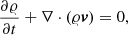 (1)
(1)
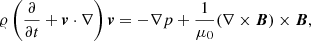 (2)
(2)
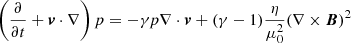 (3)
(3)
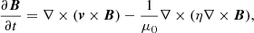 (4)
(4)
 (5)
(5)
Here, 𝜚 is a mass density, v is the flow velocity, B is the magnetic field, the adiabatic coefficient is γ = 5/3, and μ0 = 1.26 × 10⁻⁶ H m−1 is the vacuum magnetic permeability. The magnetic diffusivity, η ≈ 1 m2 s−1, is a typical value in the solar corona (see e.g. Priest 2014 page 79), and leads to a plasma resistivity value of ≈1.25 ⋅ 10−6Ωm, which is assumed to be uniform at the beginning of the calculation. The combination of the mentioned value of magnetic diffusivity and typical values of length, L0 = 106 m, and velocity, v0 = 105 m s−1, in our problem, gives us the magnetic Reynolds number, Rm = 1011, which is a reasonable value in the solar corona (see e.g. Aschwanden 2005).
Generally, the terms expressing the radiative losses, Rloss, thermal conduction, Tcond, and heating, H, should be added to the set of MHD equations. Because simulations are performed in an energetically closed model without any external sources, we assume that the radiative losses and thermal conduction are fully compensated for by the heating, H; in other words, Rloss + Tcond + H = 0 during the whole studied process.
2.2. Initial state and solutions
In our model, we have studied the turbulence caused by shear in the plasma velocities in the plasma outflow from the magnetic reconnection in solar flares. Plasma parameters were chosen, as is expected in flare reconnection outflows.
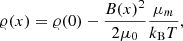
The mass density distribution was calculated from the equilibrium condition, pkin + pmag = const.:
 (6)
(6)
where 𝜚(0) = 3 ⋅ 10−11 kg ⋅ m−3 is the mass density in the centre of the current sheet, kB is the Boltzmann constant, T is the temperature, and μm = 0.6 mp is the reduced mass for the coronal plasma (see Priest 2014, page 82), where mp is the proton mass.
Our numerical box (Fig. 1) covers only the region with the plasma outflow from the magnetic reconnection. Regions of the magnetic reconnection and plasma inflow are assumed to be located somewhere below the numerical box. As is shown in (Priest 2014, page 211), in the MHD description of the magnetic reconnection, the temperature of the outflow plasma is higher than that of the inflow plasma. Thus, in the present flare case, the temperature in the outflow plasma needs to be higher than that in the inflow coronal plasma (∼1 MK). Therefore, here, as an example, we took the temperature in the outflow plasma to be T = 4 MK, which corresponds to the temperature in a small flare.
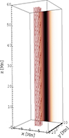 |
Fig. 1. Initial state of the model: magnetic field lines (solid red lines) starting at the bottom plane of the numerical box at the same positions as those in Fig. 3. The mass density is shown as a slice in the x–z plane at the box boundary. |
The magnetic field structure in the plasma outflow region was taken to be as simple as possible; that is, with anti-parallel magnetic field lines around the current sheet (Fig. 1) that is a transition between oppositely oriented magnetic fields, as is expected in the region of the magnetic reconnection outflow. Namely, we have assumed that below the vertically oriented numerical box (Fig. 1) the current sheet is much narrower than in the numerical box. There, the magnetic reconnection takes place and generates the plasma outflow upwards into our numerical box, where the magnetic field is described as
 (7)
(7)
where Bout = 1 G is the magnetic field at x → ∞ and wcs is the half-width of the current sheet, wcs = 3 Mm. The initial velocity of the outflowing plasma is oriented in a positive z-direction and has the Gaussian profile
![Mathematical equation: $$ \begin{aligned} { v}_z(x,{ y}) = { v}_{\rm i} \exp \left[-\frac{(x^2+{ y}^2)}{\lambda ^2}\right], \end{aligned} $$](/articles/aa/full_html/2024/12/aa49558-24/aa49558-24-eq8.gif) (8)
(8)
where λ = 1.5 Mm, and vi ≈ 27 vAlf, out ≈ 2 vS is the initial plasma flow in the current-sheet centre, with vAlf, out the external Alfvén speed and vS the sound speed, respectively. The velocity, vi, was taken as the minimum velocity for which the turbulence in the presented system was generated.
The MHD equations were solved numerically by the LARE3D, a well-tested, parallel, and open science simulation code. LARE3D is a Lagrangian-Eulerian remap numerical code that implements a staggered grid and is second-order accurate in space and time (Arber et al. 2001). The code uses the Lagrangian-remap method, splitting each timestep into a Lagrangian step followed by a remap step, which does not involve adapting the grid resolution. When the medium is deformed, the grid evolves according to the fluid flow that caused this deformation. After that, the grid is remapped onto its original state, by Van Leer gradient limiters, which (apart from the interpolation inaccuracies) does not affect the fluid variables and only transfers them to the cells of the remapped grid (see e.g. Griffies et al. 2020). In the LARE3D code, in small spatial scales of computations, where the velocity changes strongly, the artificial viscosity is implemented, as is described in Arber et al. (2001) or in the user’s manual of LARE3D.
For our numerical simulations, we used a 3D Eulerian box of size ( − 10, 10)×(−10, 10) Mm in the x and y direction and (0, 60) Mm in the vertical direction (z axis) (see Fig. 1). The box is covered by 260 × 260 × 780 grids, which gives us the smallest spatial resolution for Δx = Δy = Δz = 0.077 Mm. This grid resolution sufficiently covers the studied magnetic structures, which typically are about 1 Mm in size. Thus, the maximal grid magnetic Reynolds number is 7.7 × 10⁹. We note that such a high value could lead to numerical instability throughout the turbulent part of the simulation (for this problem, see also Thompson et al. 1985; Beg et al. 2022).
In the numerical model, we implemented periodic boundary conditions in the y and z directions. In the x direction, fixed boundary conditions were applied. Figure 1 shows the initial state of the selected magnetic field lines (solid red lines) and the mass density distribution, which is shown as a slice in the x − z plane at the boundary of the numerical box. To visualise the simulation data, we used the VisIt software package, which is a free interactive parallel visualisation and graphical analysis tool for viewing scientific data (see e.g. Childs et al. 2012).
2.3. Kinetic energy spectrum
In turbulent flows, one can find eddies of different sizes. At the beginning of the turbulent process, larger eddies are formed. Initially, these eddies gain energy from the kinetic energy of the flowing medium. During the turbulent processes, larger eddies are created, which are unstable and which then break up into a larger number of smaller vortices. Initial kinetic energy is transferred to smaller eddies, and the rest is further dissipated in the environment in the form of heat. The process of eddies breaking up, called an energy cascade, is repeated until the eddies are small enough and stable. If the flow is fully turbulent, the energy spectrum should exhibit a −5/3 decay in the so-called inertial region Kolmogorov (1941). This is known as the Kolmogorov spectrum law or the −5/3 law, and the dependence of the energy spectrum, E, of turbulent eddies in the wave number space, k, is expressed as
 (9)
(9)
where Ck ≈ 1.5 − 1.6 is called the Kolmogorov constant and ε is the power injected per unit mass into the turbulence. The inertial range, where a −5/3 slope is observed, is defined by kmin = 2π/L and kmax = 2π/l, where L and l are the maximal and minimal eddy size, respectively. We analysed the turbulence with a power spectrum analysis and estimated the inertial range (kmin–kmax; see the following section).
3. Results
Prior to performing the numerical simulations, we verified that the system remains in numerical equilibrium for the adopted grid resolution by running a test simulation without any perturbation or medium flow. The test lasted 1000 s of real (physical) time, which corresponds to 5131 time steps. During the test, there was no generation of velocities, nor were there changes in the magnetic field or mass density distribution. The temperature in the studied system remained constant. After this test, we ran the calculations with the parameters described in previous paragraphs.
In Fig. 2, we show the turbulent flow at four times: t = 493, 538, 583, and 627 s. To show the variety of flows, two different mass density values are presented in two colours (grey and blue). The initial equilibrium state was perturbed by the velocity jet of the Gaussian profile in the positive z-axis direction. At the beginning of the calculation, we also implemented small velocity perturbations in both positive and negative x directions to accelerate the creation of the turbulence process. At time ≈250 s, we observe the first ‘cores’ of the turbulence close to the z axis. At t ≈ 490 s, we observe the fully developed turbulent processes, which later evolve in time, as can be seen below.
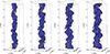 |
Fig. 2. Turbulent flow at four times: t = 493, 538, 583, and 627 s. The blue and grey colours represent two different values of mass density. |
To give an idea of how the magnetic field lines develop in the turbulent plasma flow, we present them in Fig. 3 at the same times as in Fig. 2: t = 493, 538, 583, and 627 s. Here, we can see the magnetic field lines starting at the same positions in the bottom plane of the numerical box as in the initial state (see Fig. 1).
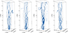 |
Fig. 3. Magnetic field lines starting at the bottom plane of the numerical box at the same positions as those in Fig. 1, at four times: t = 493, 538, 583, and 627 s. |
To show the internal structure of vortices and details of the turbulent flow, we present Fig. 4. The slices in the x − z and y − z planes are shown for the time t = 538 s, which corresponds to the second sub-figure of the turbulent flow in Fig. 2. The slices were created for the positions y = 0 Mm and x = 0 Mm, respectively. The complex structures of the turbulent flow, as well as small eddies, are present here.
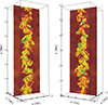 |
Fig. 4. Slices of the turbulent flow at time t = 538 s. The left part of the figure shows the slice in the x − z plane at y = 0 Mm and the right one the slice in the y − z plane at x = 0 Mm. |
In Fig. 5, the kinetic energy spectrum is presented. The spectrum was created at the time t = 627 s, when the turbulence was fully developed. To create the spectrum, we chose the place with the co-ordinates x = 2.3 Mm, y = 0 Mm where we collected the values of the velocity components along the z axis. We chose that point because the line along the z axis passes through as many vortices as possible. This is important to contain eddies of all sizes to see that the energy from the large scales to the small scales is transferred. To obtain the interval given by kmin and kmax, we selected the eddies with the largest and smallest sizes from the given point and determined these values. Using the Fourier transform, we obtained the kinetic energy depending on the wave vector, corresponding to the kinetic spectrum. The obtained spectrum is in the selected interval, which corresponds to the inertial region, the power-law form with the power-law index κ ≈ −1.655, which corresponds well to the Kolmogorov spectrum (see paragraph Sect. 2.3).
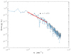 |
Fig. 5. Kinetic energy spectrum of the turbulent flow at time t = 627 s on a log-log scale. The solid red line represents the part of the spectrum with slope κ = 1.655. |
During the turbulence generation, energies in the flow change, as is shown by the lines in Figs. 6 and 7. The blue line in Fig. 6 is the normalised total energy, calculated as E△ = Etot/Etot − 0, where Etot = Ekinetic + Emagnetic + Einternal and Etot − 0 is the same sum, but at the start of the calculation (the index 0 refers to the initial value). From this graph, it can be seen that the total energy is conserved, within +0.042%. The red line shows the normalised kinetic energy, calculated as E▽ = (Ekinetic + Emagnetic − 0 + Einternal − 0)/Etot − 0. Here, we can see that the kinetic energy is at first close to the initial value and then starts to decrease, approximately around the time t ≈ 250 − 300 s. This corresponds to the time we mentioned above as the time when we observed the first turbulence cores in the system. Finally, the green line represents the sum E⊙ = (Ekinetic − 0 + Emagnetic + Einternal)/Etot − 0, which shows the changes in magnetic and internal energy. Contrary to the kinetic energy, the magnetic and internal energies increase. Because the total energy is conserved, this means that the kinetic energy in the flow is transformed into magnetic and internal energy.
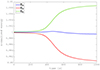 |
Fig. 6. Time evolution of normalised energies. The total energy, E△ = Etot/Etot − 0, kinetic energy, E▽ = (Ekinetic + Emagnetic − 0 + Einternal − 0)/Etot − 0, and magnetic energy, together with the internal one, E⊙ = (Ekinetic − 0 + Emagnetic + Einternal)/Etot − 0, are shown with blue, red, and green lines, respectively. The index 0 refers to the initial value. |
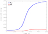 |
Fig. 7. Time evolution of normalised energies. The blue line shows the magnetic and internal energy, E° = (Emagnetic + Einternal)/(Emagnetic − 0 + Einternal − 0), and the red one represents the magnetic energy, E• = (Emagnetic + Einternal − 0)/(Emagnetic − 0 + Einternal − 0). |
To show which part of the kinetic energy turns into magnetic and internal energies, in Fig. 7 the sum of the normalised magnetic and internal energies, E° = (Emagnetic + Einternal)/(Emagnetic − 0 + Einternal − 0) (blue line), and the normalised magnetic energy, E• = (Emagnetic + Einternal − 0)/(Emagnetic − 0 + Einternal − 0) (red line), are shown. If we compare these two lines, we can see that the magnetic energy in this sum (blue line) is only a small part (about 5% from the sum). It means that most of the energy is transformed into the internal energy; therefore, into heat (about 95% of the sum). In the following subsections, we show examples of plasma velocity and magnetic structures found in the studied turbulent flow.
3.1. Example of plasma velocity vortex
In Fig. 8, for time t = 627 s and in the selected part of the numerical box, we present the plasma velocity (a,b) and magnetic vector fields (c,d), respectively. As is seen in Fig. 8a, the plasma velocity vortex has an elliptical shape. The centre of the plasma rotation vortex is at x ∼ 5 Mm and z ∼ 16 Mm. While in the x − z plane, at the vortex location, the magnetic field is distorted (Fig. 8c), in the y − z plane, at the vortex location, the magnetic field is more or less constant and oriented in a downward direction (Fig. 8d). This shows that the relationship between the magnetic and velocity fields in the turbulent flow is rather complex.
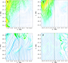 |
Fig. 8. Example of the plasma velocity vortex detected at the time 627 s. Its velocity and magnetic vector fields in the x − z and y − z planes are shown in the a, b panels and c, d panels, respectively. Vertical dashed lines in the a and c panels mean the crossing of the x − z plane by the y − z plane. On the other hand, vertical dashed lines in the b, d panels mean the crossing of the y − z plane by the x − z plane. |
3.2. Example of a magnetic field cocoon
In the left part of Fig. 9, we show one selected magnetic field line taken at t = 616 s. The starting point of this line is at the position (x = 3.175, y = −0.5, z = 0 Mm). In some locations, the line is complex (see the detail shown in the right part of Fig. 9). Owing to its form, we call this the magnetic field cocoon.
 |
Fig. 9. Example of the magnetic field cocoon at time t = 616 s. On the left is shown the selected magnetic line starting at the point (x = 3.175, y = −0.5, z = 0 Mm). On the right is a detailed view of the magnetic cocoon at the same time, expressed by the single magnetic field line. |
In Fig. 9 (right part), the magnetic field line of the magnetic cocoons is described by 30 000 points connected to the line. We note that these points are equidistant everywhere along the line. In some places, the line direction suddenly changes. This is because turbulence consists of turbulent cells of different sizes. Thus, these sudden changes in the line direction indicate boundaries between turbulent cells.
The VisIt software calculates the magnetic field lines using the multi-step Dormand-Prince method, Dormand & Prince (1980), which is recommended for calculating streamlines. We also tried to use another multi-step method, such as the Adams-Bashforth method, Ralston & Rabinowitz (2001), implemented in VisIt, but without obtaining any significant changes in the results.
The magnetic field cocoon was formed by turbulent plasma flow in interaction with the magnetic field, as is presented in another view of this structure in Fig. 10. In this figure, similarly to the previous case, the velocity (a,b) and magnetic (c,d) vector fields for the time t = 616 s are presented.
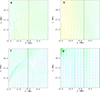 |
Fig. 10. Another view of the magnetic cocoon presented on the right of Fig. 9. Its velocity and magnetic vector fields in the x − z and y − z planes at time 616 s are shown in the a, b panels and cd panels, respectively. Vertical dashed lines in the a and c panels mean the crossing of the x − z plane by the y − z plane. On the other hand, vertical dashed lines in the b, d panels mean the crossing of the y − z plane by the x − z plane. |
3.3. Example of plasmoid
The last structures observed in our system are plasmoids. Plasmoids are magnetic structures that are created in the current sheet due to the plasmoid (tearing) instability (see e.g. Shibata & Tanuma 2001; Loureiro et al. 2007; Bárta et al. 2011). Therefore, plasmoids are found along the current sheet; that is, in our case, along the vertical plane with x = 0 Mm. An example of the plasmoid detected at time 627 s is shown in Fig. 11, especially in its panel c, where the magnetic field vectors form a circular structure. Panel d shows the magnetic field vectors crossing through this plasmoid. Non-zero vectors in this panel show that this crossing is a little bit out of the plasmoid centre, where is the zero magnetic field. The plasma flow in and around this plasmoid (Figs. 11a,b) is in an upward direction, causing this plasmoid to move upwards.
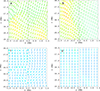 |
Fig. 11. Example of the plasmoid detected at time 627 s. Its velocity and magnetic vector fields in the x − z and y − z planes are shown in the a, b panels and c, d panels, respectively. Vertical dashed lines in the a, c panels mean the crossing of the x − z plane by the y − z plane. On the other hand, vertical dashed lines in the b, d panels mean the crossing of the y − z plane by the x − z plane. |
4. Discussion and conclusions
Turbulence is a ubiquitous process not only in astrophysics but also in other areas of plasma physics and fluid dynamics. Turbulent flow gains energy from the mean plasma flow and transports it from the largest scales to the smallest ones, where it is dissipated as heat.
Using a 3D MHD model, in which we solved a full set of the 3D time-dependent resistive and compressible MHD equations, we studied a generation of the turbulent plasma flow, its energies, and structures, such as velocity vortices, magnetic field cocoons, and plasmoids, in the system with the current sheet. This model can mimic processes in the turbulent plasma-reconnection outflow.
At the beginning of the numerical simulation, the turbulent flow is generated by a plasma velocity flow that has a Gaussian form; that is, with the maximum velocity in the system centre and a velocity approaching zero for x → ∞ and y → ∞. In our simulations, we used the initial plasma flow velocity value vi = 2vS for the configuration of the given spatial parameters. This value proved to be the most suitable for the creation of turbulent flow and the development of vortices in the investigated system. We observe eddies of various sizes in the studied system, from large ones that arise at the beginning of the simulation to smaller ones that are visible during the simulation, when the turbulence is fully developed.
Analysing a turbulent flow evolution, we found that the most of the kinetic energy of the initial plasma flow is transformed into plasma heating (about 95%) and only a small part into magnetic energy (about 5%). The turbulence in the system evolves to the saturation stage with the power-law index of the kinetic density spectrum −5/3. The magnetic energy is also saturated due to its dissipation and reconnection in small and complex magnetic field structures.
In the generated turbulent plasma flow, we detected three types of velocity and magnetic field structures: plasma velocity vortices, magnetic field cocoons, and plasmoids. These structures are important because in them the kinetic flow energy is dissipated; that is, transformed into plasma heating. Part of the kinetic flow energy is dissipated in the plasma vortices owing to the plasma viscosity, and a further part is dissipated in the magnetic cocoons and in the magnetic reconnection, forming plasmoids owing to the plasma resistivity.
The numerical simulation was performed in the high β plasma regime, where the β in the system is greater than the value at the boundary; that is, β > 2vS2/(γvAlf, out2)≈220. This value of plasma β is relatively high, which is due to a small value of the magnetic field at the edges of numerical box, and thus a small Alfvén speed. However, we have performed several numerical experiments and for this value of plasma β we have obtained the most satisfactory results regarding the formation of turbulence and the subsequently investigated velocity and magnetic structures.
The results presented in this paper show that turbulent plasma flows can effectively contribute to solar corona heating. As the turbulent processes over a wide range of spatial and temporal scales are ubiquitous in the solar wind (see e.g. (Bruno & Carbone 2005) for review), we expect that magnetic cocoons could also be found in the turbulent solar wind besides plasma velocity vortices and plasmoids.
In the future, we plan to perform numerical simulations for a lower value of plasma, β; however, we expect the velocity and magnetic structures to be similar to those in the presented case. The next plan is to study the formation of magnetic cocoons and the mutual relationship between plasma vortices and magnetic cocoons.
Acknowledgments
The authors thank the anonymous referee for constructive comments. They acknowledge support from the grant 21-16508J of the Grant Agency of the Czech Republic. MK acknowledges support from grant 22-34841S of the Grant Agency of the Czech Republic. The work in this article is part of the project DynaSun, that has received funding under the Horizon Europe programme of the European Union under grant agreement (no. 101131534). Views and opinions expressed are, however those of the author(s) only and do not necessarily reflect those of the European Union and therefore, the European Union cannot be held responsible for them.
References
- Arber, T. D., Longbottom, A. W., Gerrard, C. L., & Milne, A. M. 2001, J. Comput. Phys., 171, 151 [NASA ADS] [CrossRef] [Google Scholar]
- Aschwanden, M. J. 2005, Physics of the Solar Corona. An Introduction with Problems and Solutions (2nd edition) [Google Scholar]
- Bárta, M., Büchner, J., Karlický, M., & Skála, J. 2011, ApJ, 737, 24 [CrossRef] [Google Scholar]
- Beg, R., Russell, A. J. B., & Hornig, G. 2022, ApJ, 940, 94 [NASA ADS] [CrossRef] [Google Scholar]
- Biskamp, D. 2003, Magnetohydrodynamic Turbulence [Google Scholar]
- Bourdin, P. A., Bingert, S., & Peter, H. 2016, A&A, 589, A86 [NASA ADS] [CrossRef] [EDP Sciences] [Google Scholar]
- Bruno, R., & Carbone, V. 2005, Liv. Rev. Sol. Phys., 2, 4 [Google Scholar]
- Childs, H., Brugger, E., Whitlock, B., et al. 2012, High Performance Visualization-Enabling Extreme-Scale Scientific Insight, 357 [Google Scholar]
- Chiueh, T., & Zweibel, E. G. 1987, ApJ, 317, 900 [NASA ADS] [CrossRef] [Google Scholar]
- Dormand, J., & Prince, P. 1980, J. Comput. Appl. Math., 6, 19 [CrossRef] [MathSciNet] [Google Scholar]
- Erdélyi, R., Petrovay, K., Roberts, B., & Aschwanden, M. 2003, Turbulence, Waves and Instabilities in the Solar Plasma: Proceedings of the NATO Advanced Research Workshop on Turbulence, Waves, and Instabilities in the Solar Plasma Lillafured, Hungary 16–20 September 2002 [Google Scholar]
- Goedbloed, J. P. H., & Poedts, S. 2004, Principles of Magnetohydrodynamics [CrossRef] [Google Scholar]
- Griffies, S. M., Adcroft, A., & Hallberg, R. W. 2020, J. Adv. Model. Earth Syst., 12, e01954 [CrossRef] [Google Scholar]
- Jelínek, P., & Karlický, M. 2009, Eur. Phys. J. D, 54, 305 [CrossRef] [Google Scholar]
- Jelínek, P., Srivastava, A. K., Murawski, K., Kayshap, P., & Dwivedi, B. N. 2015, A&A, 581, A131 [NASA ADS] [CrossRef] [EDP Sciences] [Google Scholar]
- Karlický, M. 2023, Sol. Phys., 298, 95 [CrossRef] [Google Scholar]
- Karlický, M., Sobotka, M., & Jiřička, K. 1996, Sol. Phys., 168, 375 [CrossRef] [Google Scholar]
- Kayshap, P., Srivastava, A. K., Tiwari, S. K., Jelínek, P., & Mathioudakis, M. 2020, A&A, 634, A63 [NASA ADS] [CrossRef] [EDP Sciences] [Google Scholar]
- Kolmogorov, A. 1941, Akademiia Nauk SSSR Doklady, 30, 301 [Google Scholar]
- Kumar, P., & Choudhary, R. K. 2023, Sol. Phys., 298, 128 [NASA ADS] [CrossRef] [Google Scholar]
- Lapenta, G. 2019, Nuovo Cimento C Geophysics Space Physics C, 42, 22 [NASA ADS] [Google Scholar]
- Larosa, T. N., Moore, R. L., & Shore, S. N. 1994, ApJ, 425, 856 [NASA ADS] [CrossRef] [Google Scholar]
- Liu, W., Petrosian, V., Dennis, B. R., & Jiang, Y. W. 2008, ApJ, 676, 704 [NASA ADS] [CrossRef] [Google Scholar]
- Loureiro, N. F., Schekochihin, A. A., & Cowley, S. C. 2007, Phys. Plasmas, 14, 100703 [NASA ADS] [CrossRef] [Google Scholar]
- Nakariakov, V. M., Pilipenko, V., Heilig, B., et al. 2016, Space Sci. Rev., 200, 75 [Google Scholar]
- Petrosyan, A., Balogh, A., Goldstein, M. L., et al. 2010, Space Sci. Rev., 156, 135 [NASA ADS] [CrossRef] [Google Scholar]
- Priest, E. 2014, Magnetohydrodynamics of the Sun [Google Scholar]
- Ralston, A., & Rabinowitz, P. 2001, A First Course in Numerical Analysis, Dover books on mathematics (Dover Publications) [Google Scholar]
- Rappazzo, A. F., Velli, M., Einaudi, G., & Dahlburg, R. B. 2008, ApJ, 677, 1348 [Google Scholar]
- Rieutord, M. 2015, Fluid Dynamics: An Introduction [Google Scholar]
- Ruan, W., Yan, L., & Keppens, R. 2023, ApJ, 947, 67 [NASA ADS] [CrossRef] [Google Scholar]
- Shibata, K., & Tanuma, S. 2001, Earth Planets Space, 53, 473 [NASA ADS] [CrossRef] [Google Scholar]
- Shibata, K., Nitta, N., Strong, K. T., et al. 1994, ApJ, 431, L51 [Google Scholar]
- Thompson, H. D., Webb, B. W., & Hoffman, J. D. 1985, Int. J. Numer. Methods Fluids, 5, 305 [NASA ADS] [CrossRef] [Google Scholar]
- Tziotziou, K., Scullion, E., Shelyag, S., et al. 2023, Space Sci. Rev., 219, 1 [NASA ADS] [CrossRef] [Google Scholar]
- Visconti, G., & Ruggieri, P. 2020, Fluid Dynamics: Fundamentals and Applications [CrossRef] [Google Scholar]
- Vörös, Z., Sasunov, Y. L., Semenov, V. S., et al. 2014, ApJ, 797, L10 [CrossRef] [Google Scholar]
- Zhou, M., Man, H. Y., Deng, X. H., et al. 2021, Geophys. Res. Lett., 48, e91215 [NASA ADS] [Google Scholar]
All Figures
|
Fig. 1. Initial state of the model: magnetic field lines (solid red lines) starting at the bottom plane of the numerical box at the same positions as those in Fig. 3. The mass density is shown as a slice in the x–z plane at the box boundary. |
| In the text | |
|
Fig. 2. Turbulent flow at four times: t = 493, 538, 583, and 627 s. The blue and grey colours represent two different values of mass density. |
| In the text | |
|
Fig. 3. Magnetic field lines starting at the bottom plane of the numerical box at the same positions as those in Fig. 1, at four times: t = 493, 538, 583, and 627 s. |
| In the text | |
|
Fig. 4. Slices of the turbulent flow at time t = 538 s. The left part of the figure shows the slice in the x − z plane at y = 0 Mm and the right one the slice in the y − z plane at x = 0 Mm. |
| In the text | |
|
Fig. 5. Kinetic energy spectrum of the turbulent flow at time t = 627 s on a log-log scale. The solid red line represents the part of the spectrum with slope κ = 1.655. |
| In the text | |
|
Fig. 6. Time evolution of normalised energies. The total energy, E△ = Etot/Etot − 0, kinetic energy, E▽ = (Ekinetic + Emagnetic − 0 + Einternal − 0)/Etot − 0, and magnetic energy, together with the internal one, E⊙ = (Ekinetic − 0 + Emagnetic + Einternal)/Etot − 0, are shown with blue, red, and green lines, respectively. The index 0 refers to the initial value. |
| In the text | |
|
Fig. 7. Time evolution of normalised energies. The blue line shows the magnetic and internal energy, E° = (Emagnetic + Einternal)/(Emagnetic − 0 + Einternal − 0), and the red one represents the magnetic energy, E• = (Emagnetic + Einternal − 0)/(Emagnetic − 0 + Einternal − 0). |
| In the text | |
|
Fig. 8. Example of the plasma velocity vortex detected at the time 627 s. Its velocity and magnetic vector fields in the x − z and y − z planes are shown in the a, b panels and c, d panels, respectively. Vertical dashed lines in the a and c panels mean the crossing of the x − z plane by the y − z plane. On the other hand, vertical dashed lines in the b, d panels mean the crossing of the y − z plane by the x − z plane. |
| In the text | |
|
Fig. 9. Example of the magnetic field cocoon at time t = 616 s. On the left is shown the selected magnetic line starting at the point (x = 3.175, y = −0.5, z = 0 Mm). On the right is a detailed view of the magnetic cocoon at the same time, expressed by the single magnetic field line. |
| In the text | |
|
Fig. 10. Another view of the magnetic cocoon presented on the right of Fig. 9. Its velocity and magnetic vector fields in the x − z and y − z planes at time 616 s are shown in the a, b panels and cd panels, respectively. Vertical dashed lines in the a and c panels mean the crossing of the x − z plane by the y − z plane. On the other hand, vertical dashed lines in the b, d panels mean the crossing of the y − z plane by the x − z plane. |
| In the text | |
|
Fig. 11. Example of the plasmoid detected at time 627 s. Its velocity and magnetic vector fields in the x − z and y − z planes are shown in the a, b panels and c, d panels, respectively. Vertical dashed lines in the a, c panels mean the crossing of the x − z plane by the y − z plane. On the other hand, vertical dashed lines in the b, d panels mean the crossing of the y − z plane by the x − z plane. |
| In the text | |
Current usage metrics show cumulative count of Article Views (full-text article views including HTML views, PDF and ePub downloads, according to the available data) and Abstracts Views on Vision4Press platform.
Data correspond to usage on the plateform after 2015. The current usage metrics is available 48-96 hours after online publication and is updated daily on week days.
Initial download of the metrics may take a while.