| Issue |
A&A
Volume 691, November 2024
|
|
|---|---|---|
| Article Number | L20 | |
| Number of page(s) | 10 | |
| Section | Letters to the Editor | |
| DOI | https://doi.org/10.1051/0004-6361/202451949 | |
| Published online | 22 November 2024 | |
Letter to the Editor
Seismic differences between solar magnetic cycles 23 and 24 for low-degree modes
1
Université Paris-Saclay, Université Paris Cité, CEA, CNRS, AIM, 91191 Gif-sur-Yvette, France
2
INAF – Osservatorio Astrofisico di Catania, Via S. Sofia, 78, 95123 Catania, Italy
3
Université Paris Cité, Université Paris-Saclay, CEA, CNRS, AIM, 91191 Gif-sur-Yvette, France
4
Université Côte d’Azur, Observatoire de la Côte d’Azur, CNRS, Laboratoire Lagrange, Nice, France
5
National Solar Observatory, 3665 Discovery Drive, Boulder, CO 80303, USA
6
Instituto de Astrofísica de Canarias (IAC), E-38205 La Laguna, Tenerife, Spain
7
Universidad de La Laguna (ULL), Departamento de Astrofísica, E-38206 La Laguna, Tenerife, Spain
⋆ Corresponding author; rgarcia@cea.fr
Received:
21
August
2024
Accepted:
25
October
2024
Solar magnetic activity follows regular cycles of about 11 years with an inversion of polarity in the poles every ∼22 years. This changing surface magnetism impacts the properties of the acoustic modes. The acoustic mode frequency shifts are a good proxy of the magnetic cycle. In this Letter we investigate solar magnetic activity cycles 23 and 24 through the evolution of the frequency shifts of low-degree modes (ℓ = 0, 1, and 2) in three frequency bands. These bands probe properties between 74 and 1575 km beneath the surface. The analysis was carried out using observations from the space instrument Global Oscillations at Low Frequency and the ground-based Birmingham Solar Oscillations Network and Global Oscillation Network Group. The frequency shifts of radial modes suggest that changes in the magnetic field amplitude and configuration likely occur near the Sun’s surface rather than near its core. The maximum shifts of solar cycle 24 occurred earlier at mid and high latitudes (relative to the equator) and about 1550 km beneath the photosphere. At this depth but near the equator, this maximum aligns with the surface activity but has a stronger magnitude. At around 74 km deep, the behaviour near the equator mirrors the behaviour at the surface, while at higher latitudes, it matches the strength of cycle 23.
Key words: methods: data analysis / Sun: activity / Sun: helioseismology
© The Authors 2024
 Open Access article, published by EDP Sciences, under the terms of the Creative Commons Attribution License (https://creativecommons.org/licenses/by/4.0), which permits unrestricted use, distribution, and reproduction in any medium, provided the original work is properly cited.
This article is published in open access under the Subscribe to Open model. Subscribe to A&A to support open access publication.
1. Introduction
Main-sequence solar-like stars have a convective envelope where the interaction between convection, rotation, and magnetic fields results in a magnetic activity cycle (e.g. Brun & Browning 2017). However, the reasons why some stars with similar fundamental properties show very different magnetic activity levels are still unclear (e.g. Baliunas et al. 1995; Egeland 2017; See et al. 2021; Santos et al. 2024). Large spectroscopic surveys, such as the one led at the Mount Wilson Observatory (Wilson 1978) or at Lowell Observatory (Hall et al. 2007), and surveys that use spectropolarimetry (e.g. Marsden et al. 2014) or space-based photometric observations (García et al. 2014; McQuillan et al. 2014; Mathur et al. 2014; Reinhold et al. 2017; Santos et al. 2019, 2021) show a large diversity of magnetic variability (cyclic, flat, or variable stars; Baliunas & Vaughan 1985). Recent studies even suggest that the magnetic solar cycle might soon stop or change its nature (e.g. Metcalfe 2018; McIntosh et al. 2019; Noraz et al. 2022, 2024). Thus, it is necessary to keep monitoring the temporal evolution of the Sun with a broad set of observables at different heights, from the corona to the sub-surface layers, to impose tighter constraints on current physical models.
Over the last 50 years, helioseismology, and more recently asteroseismology, has been able to probe the properties of solar and stellar interiors with high precision (e.g. García & Ballot 2019; Christensen-Dalsgaard 2021). Surface magnetism perturbs the properties of the acoustic oscillation modes (p modes) in several ways. In particular, p-mode properties are affected by magnetic activity; this was first detected in the Sun (e.g. Pallé et al. 1989; Elsworth et al. 1990; Anguera Gubau et al. 1992; Jiménez-Reyes et al. 2003; Tripathy et al. 2010; Howe et al. 2017, 2022a) and later in solar-like stars (e.g. García et al. 2010; Salabert et al. 2011a, 2016; Mathur et al. 2013, 2019; Kiefer et al. 2017; Karoff et al. 2018; Santos et al. 2018). Mode frequencies are shifted and correlated with the magnetic cycle, while the mode amplitudes are anti-correlated. These frequency shifts can modify the age estimation of a star like the Sun, with variations of up to 6.5% between solar minima and maxima (Bétrisey et al. 2024). Studies focused on the low-activity phase between cycles also suggest complicated spatial distributions of magnetic fields beneath the solar surface (Salabert et al. 2009; Jain et al. 2022).
Recently, a detailed seismic analysis that included medium- and high-degree modes collected by the Solar Oscillation Imager/Michelson Doppler Imager (SOI/MDI; Scherrer et al. 1995), the Helioseismic and Magnetic Imager (HMI; Scherrer et al. 2012), and the Global Oscillation Network Group (GONG; Harvey et al. 1996) by Basu (2021) has revealed significant changes in the solar convection zone (and even below), indicating possible small changes in the position of the tachocline. Moreover, Inceoglu et al. (2021) studied solar quasi-biennial oscillations (QBOs; Sakurai 1979) in the rotation rate residuals and conclude that QBO-like signals were present at different latitudinal bands, with their amplitudes increasing with depth. In addition, Kurtz et al. (2014) showed that the quasi-biennial variability in the solar interior depended on the cycle (see also Mehta et al. 2022). In addition, a recent study by Jain et al. (2023) found different QBO periods in cycles 23 and 24.
Unfortunately, in the case of the asteroseismology of solar-like stars, only low-degree modes can be detected, and the capabilities to diagnose the impact of the surface magnetic activity at different layers are limited. Nevertheless, using these low-degree p modes, it is still possible to evaluate structural perturbations in the ∼3000 km beneath the surface (Basu et al. 2012; Salabert et al. 2015; Jain et al. 2018). In this work we investigated the solar seismic signatures of cycles 23 and 24 (from 1996 to 2020) through the evolution of averaged frequency shifts, ⟨δν⟩, of low-degree modes (ℓ = 0, 1, and 2) in different frequency ranges. This allowed us to study, on one hand, the dependence on latitude because radial modes are more sensitive to mid and high latitudes, while dipolar and quadrupolar sectoral modes (ℓ = |m|) are more sensitive towards the equator and with increasing ℓ (see Jiménez-Reyes et al. 2004a, and Fig. 3 in Chaplin & Basu 2014). On the other hand, by averaging the ⟨δν⟩ in different frequency bands, we were able to study the sensitivity of the magnetic perturbation to depth. In this context, we note that Simoniello et al. (2016) analysed intermediate- and high-degree modes of GONG data for a part of cycle 23 using different frequency ranges and harmonic degrees and conclude that the frequency shifts behave differently at low and high latitudes.
The layout of this Letter is as follows. In Sect. 2 we present the observations and the procedure for extracting the p-mode frequency shifts. In Sect. 3 we present the results and discuss them in Sect. 4.
2. Observations and data analysis
We used three different datasets of velocity measurements. The first one was collected by the Global Oscillations at Low Frequency (GOLF) instrument1 (Gabriel et al. 1995, 1997) on board the Solar and Heliospheric Observatory (SoHO; Domingo et al. 1995). We obtained 24.5 years of continuous data – from April 11, 1996, until September 4, 2020 – of Doppler velocity time series following García et al. (2005) and ensuring a proper timing of the measurements (for more details, see Appourchaux et al. 2018; Breton et al. 2022a). The second dataset was collected with the Birmingham Solar Oscillation Network (BiSON2; Hale et al. 2016) starting at the same time as GOLF but extending only to April 4, 2020 and corrected following the procedure described in Davies et al. (2014). The third dataset is composed of Doppler velocity measurements from the GONG network3 (Jain et al. 2021). The series in this third dataset start on May 7, 1995, and are available through October 9, 2020, with a median duty cycle value of 87% (varying between 78% and 92%).
Both the GOLF and BiSON datasets are divided into consecutive sub-series of 365 days shifted by 91.25 days, while the GONG dataset comprises 360 days shifted by 72 days. Series with a duty cycle below 80%, 70%, and 56% respectively for GOLF, GONG, and BiSON were removed. 15 consecutive radial orders between 1800 μHz and 3790 μHz were fitted (as explained in Appendix A) following a traditional, deterministic, maximum likelihood (ML) algorithm or through the apollinaire module4 (Breton et al. 2022b), which implements a Markov chain Monte Carlo (MCMC) Bayesian sampling of the model parameter posterior distribution (Foreman-Mackey et al. 2013). The lowest fitted radial order is n = 12 for ℓ = 0 and 1, and n = 11 for ℓ = 2. We did not use ℓ = 3 modes in our analysis because of their low signal-to-noise ratio in Sun-as-a-star data.
Temporal variations in mode frequencies, ⟨δν⟩, were defined as the differences between the frequencies observed at a given time and the average of the frequencies of years 1996–1997 (independent series 1 and 5), corresponding to the minimum of activity of cycles 22–23. The frequency-shift errors were computed as
Once the frequency shifts were obtained, they were averaged in three different frequency bands following Basu et al. (2012): (i) the low-frequency band (LFB) from 1800 to 2450 μHz; (ii) the medium-frequency band (MFB) from 2450 to 3110 μHz; and (iii) the high-frequency band (HFB) from 3110 to 3790 μHz. The formal uncertainties resulting from the peak-fitting analysis were used as weights in the computation of the averages of the different degree modes and frequency bands. The resultant ⟨δνℓ = 0, 1, 2⟩ for the three instruments are given in Appendix B (Tables B.1, B.2, and B.3). Using model BS05 from Bahcall & Serenelli (2005), we computed the average sensitivity for each degree in each frequency band. The results are shown in Table 1 and Fig. 1. Since the kernels for individual (n, ℓ) modes have different depth sensitivities, we calculated these values by averaging them over all the n and ℓ values in each selection taken from the observations. Our kernels are slightly different from those in Basu et al. (2012) and Salabert et al. (2015) because the modes averaged in each frequency band are not the same. For example, Basu et al. (2012) used the same number of overtones (i.e. four) in all three frequency ranges, while we used five consecutive radial orders in each category. This led to the use of a different set of modes in this study and hence a different depth sensitivity.
Depths from the surface of the sensitivity kernels.
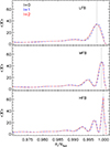 |
Fig. 1. Integrated sensitivity, ⟨𝒦⟩, as a function of the relative radius for the LFB, MFB, and HFB (top, middle, and bottom panels, respectively) from the BS05 model in Bahcall & Serenelli (2005). Vertical dotted lines indicate the depth of the sensitivity kernels for ℓ = 0 modes. |
Finally, because we are interested in comparing solar cycles 23 and 24, we removed the contribution of the QBO (e.g. Fletcher et al. 2010; Jain et al. 2011; Simoniello et al. 2012) by smoothing the data with a boxcar of 2.5 years. To reduce any border effects associated with the filtering, we extended the ⟨δν⟩ by half of the filter width, assuming them to be symmetric with respect to the beginning and the end of the series.
In addition, mean values of daily measurements of the 10.7 cm radio flux5, F10.7, were used as a proxy of the solar surface activity since it has been shown that this magnetic activity proxy is the best correlated with the mean frequency shifts (e.g. Jain et al. 2009; Howe et al. 2017). The same 2.5-a-boxcar filter was applied to remove the QBO contribution from this proxy. Using the filtered F10.7, we determined the reference dates for the maximum of cycles 23 and 24 and the minimum in between, respectively March 2001, January 2014, and July 2008.
By comparing the mode parameters from MDI and HMI, which used two different spectral lines (Ni I 676.8 nm and Fe I 617.3 nm, respectively), Larson & Schou (2018) found that differences in frequencies and splitting coefficients were not significant. In addition, no differences were found when comparing the temporal evolution of p-mode parameters of GOLF and BiSON (Jiménez-Reyes et al. 2004b) except for the mode asymmetry (Jiménez-Reyes et al. 2007). Thus, we conclude that our results should not be affected by the fact that they are based on the study of the temporal evolution of ⟨δν⟩ involving different instruments observing the signals at slightly different heights.
3. Results: Temporal evolution of GOLF frequency shifts
The temporal evolution of the 2.5-a-boxcar smoothed ⟨δν⟩ from GOLF is shown in Fig. 2. Each column corresponds to a different mode (ℓ = 0, 1, and 2), and each row corresponds to the aforementioned frequency bands. A figure containing the non-smoothed ⟨δν⟩ is shown in Appendix C. In each panel, the F10.7 radio flux is scaled to the ⟨δν⟩ using the rising phase of cycle 23. For the sake of clarity and because the qualitative results are the same for the three instruments, only the GOLF results are presented. In Appendix D, results obtained with the other two datasets are compared and discussed.
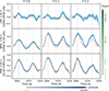 |
Fig. 2. Temporal evolution of the averaged and smoothed GOLF frequency shifts (⟨δν⟩, dark blue lines) of ℓ = 0, 1, and 2 modes (left, central, and right panels respectively). The top, middle, and bottom rows correspond to the three frequency bands considered in the analysis: 1800–2450 (LFB), 2450–3110 (MFB), and 3110–3790 μHz (HFB), respectively. Light blue regions represent the errors in ⟨δν⟩. Orange lines depict the scaled smoothed F10.7 magnetic proxy. Vertical dashed and dot-dashed lines depict the maxima of cycles 23 and 24 and the minimum in between. The horizontal blue arrow indicates the change in sensitivity from the pole to the equator, and the vertical green arrow depicts the maximum sensitivity to the depth of the subsurface layers. |
Overall, the ⟨δν⟩ follow the evolution of the F10.7, but there are some notable differences:
-
The rising phase of cycle 24 in the LFB ⟨δνℓ = 0⟩ is reached in 2012, two years earlier than F10.7.
-
Cycle 24 is known to have a lower amplitude than cycle 23, as shown for example by Howe et al. (2022a) and by the F10.7. In this respect, ⟨δν⟩ modulations have surprisingly large amplitudes in cycle 24 for some frequency bands and degrees, ℓ. The amplitude of the LFB ⟨δνℓ = 1⟩ of cycle 24 is nearly twice that of cycle 23, while for the MFB ⟨δνℓ = 2⟩, the amplitude of cycle 24 is comparable to that of cycle 23. In all of these cases, the amplitude of cycle 24 is clearly higher than that of the F10.7. The MFB ⟨δνℓ = 0⟩ reaches its minimum between the two cycles around a year earlier than the F10.7.
-
The MFB ⟨δνℓ = 1⟩ and HFB ⟨δνℓ = 0⟩ are both greater than F10.7 in cycle 24.
-
With larger and larger error bars in the LFB ⟨δνℓ = 2⟩ since 2005, due to the lower counting rates of the GOLF instrument, we cannot extract information on cycle 24.
-
For the remaining three cases, the MFB ⟨δνℓ = 0⟩ and the HFB ⟨δνℓ = 1⟩ and ⟨δνℓ = 2⟩, they closely follow F10.7.
4. Discussion
Recent seismic analyses of averaged frequency shifts for both low-degree modes (Howe et al. 2022a) and medium- and high-degree modes (Jain et al. 2022) show that the influence of the magnetic perturbations on the acoustic modes are different during consecutive solar cycles. Although it is usually assumed that the main perturbations on the mode frequencies are located in the sub-surface layers, it has also been speculated that a fossil magnetic field in the core of the Sun could play a crucial role in the generation of the solar magnetic cycle and thus could also modify the properties of the acoustic modes (e.g. Sonett 1983; Mursula et al. 2001). Such magnetic fields have not been observed in main-sequence solar-like stars yet, but they could modify the structure of stellar oscillations (e.g. Goode & Thompson 1992; Loi & Papaloizou 2018; Bugnet et al. 2021). They have been observed in the core of red giants (Li et al. 2022, 2024; Deheuvels et al. 2023).
As discussed in the previous section, the maximum of the ⟨δνℓ = 0⟩ in cycle 24 arrives two years earlier in the LFB. This means that something changed between the two cycles at a depth of ∼1550 km below the photosphere (see Table 1 and Fig. 1). The dominant perturbation in the LFB ⟨δνℓ = 0⟩ is weighted towards mid to high latitudes, while the maximum of ⟨δνℓ = 1⟩ is synchronised with F10.7 except in regions close to the equator, where ⟨δνℓ = 1⟩ are the most sensitive. Therefore, in cycle 24, the magnetic perturbation modifying ⟨δνℓ = 0⟩ reaches an extended 4-a maximum earlier (∼2010) at high latitudes and at a depth of ∼1550 km beneath the surface. This perturbation reaches shallower layers (> 1402 km) at the same time as the photosphere, with a maximum of around ∼2014. At these mid and high latitudes, just below the photosphere (∼74 km), the HFB of ⟨δνℓ = 0⟩ shows stronger variations than the surface activity represented by the F10.7 in cycle 24. Based on our analysis of the radial modes, we do not find evidence supporting that the changes comes from an hypothetical magnetic field in the core of the Sun as the MFB ⟨δνℓ = 0⟩ seems to follow the evolution of F10.7 very closely. The fact that all the radial modes reach the centre rules out a change coming from the core of the Sun. Only the upper turning points are different. Thus, the change in the perturbation should be located at the subsurface layers, which likely have a complicated vertical structure.
Near the solar equator, we see that the LFB of ⟨δνℓ = 1⟩ is stronger in cycle 24 than in cycle 23. The perturbation of the dipolar modes at ∼1402 km is larger in the later cycle. The differences in the ⟨δν⟩ of the ℓ = 1 and 2 modes compared to the F10.7 in cycle 24 are also large in the MFB. In this cycle, the maximum of the dipolar ⟨δν⟩ is slightly smaller than in cycle 23, while it is larger for the quadrupolar modes. That means that the perturbation is larger very close to the equator since the difference in the depth is very small (∼412 versus ∼487 km). Finally, very close to the surface (∼74–75 km), the behaviour of ⟨δν⟩ is almost identical to the surface activity. Despite the different frequency bands and mode degrees, we find similar qualitative results regarding the dependence of the progression of solar cycle 23 to those obtained by Simoniello et al. (2016).
5. Conclusions
Similar to previous studies using intermediate- and high-degree modes (e.g. Howe et al. 2022b, and references therein), the present study allowed us to trace how the solar-cycle-induced perturbations evolve with time, latitude, and depth using low-degree modes during solar cycles 23 and 24, and with three different instruments, GOLF, BiSON, and GONG. Our first conclusion is that the temporal evolution of the radial-mode frequency shifts suggests that these changes most likely did not occur in the solar core but rather close to the surface. The second conclusion is that the maximum shifts of cycle 24 seem to arrive earlier at mid and high latitudes compared to cycle 23 and at a depth of around 1550 km. At this depth and near the equator, the maximum of cycle 24 is synchronised with the surface, but the magnitude is stronger than at the surface. Finally, in a band around 74 km beneath the surface and near the equator, the behaviour is similar to that at the surface, while at higher latitudes it matches the strength of cycle 23. The results obtained with the three instruments are in close agreement in most of the cases. However, as shown in Appendix B, the main difference is the presence of a clear QBO pattern in the GONG LFB of ⟨δνℓ = 0⟩ that is not seen in the integrated-light instruments. The smoothed frequency shift also behaves differently, closely following the F10.7. Our analysis can also be used to test new theories on the origin of the solar dynamo (Vasil et al. 2024).
Data availability
Full Tables B.1, B.2, and B.3 are available at the CDS via anonymous ftp to cdsarc.cds.unistra.fr (130.79.128.5) or via https://cdsarc.cds.unistra.fr/viz-bin/cat/J/A+A/691/L20
Acknowledgments
We thank J. Ballot and F. Pérez Hernández for useful comments and discussions. K.J. thanks Sarbani Basu for providing the standard solar model values. The GOLF instrument on board SoHO is a cooperative effort of many individuals, to whom we are indebted. SoHO is a project of international collaboration between ESA and NASA. BiSON is funded by the UK Science and Technology Facilities Council (STFC). This work also utilises GONG data obtained by the NSO Integrated Synoptic Program, managed by the National Solar Observatory, which is operated by the Association of Universities for Research in Astronomy (AURA), Inc. under a cooperative agreement with the National Science Foundation and with contribution from the National Oceanic and Atmospheric Administration. The GONG network of instruments is hosted by the Big Bear Solar Observatory, High Altitude Observatory, Learmonth Solar Observatory, Udaipur Solar Observatory, Instituto de Astrofísica de Canarias, and Cerro Tololo Interamerican Observatory. R.A.G., S.N.B., and E.P. acknowledge the support from the GOLF and PLATO Centre National D’Études Spatiales grants. S.N.B acknowledges support from PLATO ASI-INAF agreement n. 2015-019-R.1-2018. S.M. acknowledges support by the Spanish Ministry of Science and Innovation with the Ramon y Cajal fellowship number RYC-2015-17697 and the grant number PID2019-107187GB-I00, and through AEI under the Severo Ochoa Centres of Excellence Programme 2020–2023 (CEX2019-000920-S). S.C.T. and K.J. acknowledge partial funding support from the NASA DRIVE Science Center COFFIES Phase II CAN 80NSSC22M0162. Software: AstroPy (Astropy Collaboration 2013, 2018), Matplotlib (Hunter 2007), NumPy (van der Walt et al. 2011), SciPy (Jones et al. 2001), pandas (Wes McKinney 2010; The pandas development team 2020), emcee (Foreman-Mackey et al. 2013), apollinaire (Breton et al. 2022b), Interactive Data Language (IDL).
References
- Anderson, E. R., Duvall, T. L., Jr., & Jefferies, S. M. 1990, ApJ, 364, 699 [NASA ADS] [CrossRef] [Google Scholar]
- Anguera Gubau, M., Palle, P. L., Perez Hernandez, F., Regulo, C., & Roca Cortes, T. 1992, A&A, 255, 363 [NASA ADS] [Google Scholar]
- Appourchaux, T., Boumier, P., Leibacher, J. W., & Corbard, T. 2018, A&A, 617, A108 [NASA ADS] [CrossRef] [EDP Sciences] [Google Scholar]
- Astropy Collaboration (Robitaille, T. P., et al.) 2013, A&A, 558, A33 [NASA ADS] [CrossRef] [EDP Sciences] [Google Scholar]
- Astropy Collaboration (Price-Whelan, A. M., et al.) 2018, AJ, 156, 123 [Google Scholar]
- Bahcall, J. N., & Serenelli, A. M. 2005, ApJ, 626, 530 [NASA ADS] [CrossRef] [Google Scholar]
- Baliunas, S. L., & Vaughan, A. H. 1985, ARA&A, 23, 379 [NASA ADS] [CrossRef] [Google Scholar]
- Baliunas, S. L., Donahue, R. A., Soon, W. H., et al. 1995, ApJ, 438, 269 [Google Scholar]
- Basu, S. 2021, ApJ, 917, 45 [NASA ADS] [CrossRef] [Google Scholar]
- Basu, S., Broomhall, A.-M., Chaplin, W. J., & Elsworth, Y. 2012, ApJ, 758, 43 [NASA ADS] [CrossRef] [Google Scholar]
- Benomar, O., Appourchaux, T., & Baudin, F. 2009, A&A, 506, 15 [NASA ADS] [CrossRef] [EDP Sciences] [Google Scholar]
- Bétrisey, J., Farnir, M., Breton, S. N., et al. 2024, A&A, 688, L17 [NASA ADS] [CrossRef] [EDP Sciences] [Google Scholar]
- Breton, S. N., Pallé, P. L., García, R. A., et al. 2022a, A&A, 658, A27 [NASA ADS] [CrossRef] [EDP Sciences] [Google Scholar]
- Breton, S. N., García, R. A., Ballot, J., Delsanti, V., & Salabert, D. 2022b, A&A, 663, A118 [NASA ADS] [CrossRef] [EDP Sciences] [Google Scholar]
- Brun, A. S., & Browning, M. K. 2017, Liv. Rev. Sol. Phys., 14, 4 [Google Scholar]
- Bugnet, L., Prat, V., Mathis, S., et al. 2021, A&A, 650, A53 [NASA ADS] [CrossRef] [EDP Sciences] [Google Scholar]
- Chaplin, W. J., & Basu, S. 2014, Space Sci. Rev., 186, 437 [NASA ADS] [CrossRef] [Google Scholar]
- Christensen-Dalsgaard, J. 2021, Liv. Rev. Sol. Phys., 18, 2 [NASA ADS] [CrossRef] [Google Scholar]
- Davies, G. R., Chaplin, W. J., Elsworth, Y., & Hale, S. J. 2014, MNRAS, 441, 3009 [NASA ADS] [CrossRef] [Google Scholar]
- Deheuvels, S., Li, G., Ballot, J., & Lignières, F. 2023, A&A, 670, L16 [NASA ADS] [CrossRef] [EDP Sciences] [Google Scholar]
- Domingo, V., Fleck, B., & Poland, A. I. 1995, Sol. Phys., 162, 1 [Google Scholar]
- Egeland, R. 2017, Ph.D. Thesis, Montana State University, Bozeman, Montana, USA [Google Scholar]
- Elsworth, Y., Howe, R., Isaak, G. R., McLeod, C. P., & New, R. 1990, Nature, 345, 322 [NASA ADS] [CrossRef] [Google Scholar]
- Fletcher, S. T., Broomhall, A., Salabert, D., et al. 2010, ApJ, 718, L19 [NASA ADS] [CrossRef] [Google Scholar]
- Foreman-Mackey, D., Hogg, D. W., Lang, D., & Goodman, J. 2013, PASP, 125, 306 [Google Scholar]
- Gabriel, A. H., Grec, G., Charra, J., et al. 1995, Sol. Phys., 162, 61 [Google Scholar]
- Gabriel, A. H., Charra, J., Grec, G., et al. 1997, Sol. Phys., 175, 207 [NASA ADS] [CrossRef] [Google Scholar]
- García, R. A., & Ballot, J. 2019, Liv. Rev. Sol. Phys., 16, 4 [Google Scholar]
- García, R. A., Turck-Chièze, S., Boumier, P., et al. 2005, A&A, 442, 385 [NASA ADS] [CrossRef] [EDP Sciences] [Google Scholar]
- García, R. A., Mathur, S., Salabert, D., et al. 2010, Science, 329, 1032 [Google Scholar]
- García, R. A., Ceillier, T., Salabert, D., et al. 2014, A&A, 572, A34 [NASA ADS] [CrossRef] [EDP Sciences] [Google Scholar]
- Goode, P. R., & Thompson, M. J. 1992, ApJ, 395, 307 [Google Scholar]
- Hale, S. J., Howe, R., Chaplin, W. J., Davies, G. R., & Elsworth, Y. P. 2016, Sol. Phys., 291, 1 [NASA ADS] [CrossRef] [Google Scholar]
- Hall, J. C., Lockwood, G. W., & Skiff, B. A. 2007, AJ, 133, 862 [Google Scholar]
- Harvey, J. W., Hill, F., Hubbard, R., et al. 1996, Science, 272, 1284 [CrossRef] [Google Scholar]
- Howe, R., Davies, G. R., Chaplin, W. J., et al. 2017, MNRAS, 470, 1935 [NASA ADS] [CrossRef] [Google Scholar]
- Howe, R., Chaplin, W. J., Elsworth, Y. P., Hale, S. J., & Nielsen, M. B. 2022a, MNRAS, 514, 3821 [CrossRef] [Google Scholar]
- Howe, R., Chaplin, W. J., Christensen-Dalsgaard, J., Elsworth, Y. P., & Schou, J. 2022b, RNAAS, 6, 261 [NASA ADS] [Google Scholar]
- Hunter, J. D. 2007, Comput. Sci. Eng., 9, 90 [NASA ADS] [CrossRef] [Google Scholar]
- Inceoglu, F., Howe, R., & Loto’aniu, P. T. M. 2021, ApJ, 920, 49 [NASA ADS] [CrossRef] [Google Scholar]
- Jain, K., Tripathy, S. C., & Hill, F. 2009, ApJ, 695, 1567 [NASA ADS] [CrossRef] [Google Scholar]
- Jain, K., Tripathy, S. C., & Hill, F. 2011, ApJ, 739, 6 [NASA ADS] [CrossRef] [Google Scholar]
- Jain, K., Tripathy, S., Hill, F., et al. 2018, IAU Symp., 340, 27 [CrossRef] [Google Scholar]
- Jain, K., Tripathy, S. C., Hill, F., & Pevtsov, A. A. 2021, PASP, 133, 105001 [NASA ADS] [CrossRef] [Google Scholar]
- Jain, K., Jain, N., Tripathy, S. C., & Dikpati, M. 2022, ApJ, 924, L20 [NASA ADS] [CrossRef] [Google Scholar]
- Jain, K., Chowdhury, P., & Tripathy, S. C. 2023, ApJ, 959, 16 [NASA ADS] [CrossRef] [Google Scholar]
- Jiménez-Reyes, S. J., García, R. A., Jiménez, A., & Chaplin, W. J. 2003, ApJ, 595, 446 [CrossRef] [Google Scholar]
- Jiménez-Reyes, S. J., García, R. A., Chaplin, W. J., & Korzennik, S. G. 2004a, ApJ, 610, L65 [CrossRef] [Google Scholar]
- Jiménez-Reyes, S. J., Chaplin, W. J., Elsworth, Y., & García, R. A. 2004b, ApJ, 604, 969 [CrossRef] [Google Scholar]
- Jiménez-Reyes, S. J., Chaplin, W. J., Elsworth, Y., et al. 2007, ApJ, 654, 1135 [CrossRef] [Google Scholar]
- Jones, E., Oliphant, T., Peterson, P., et al. 2001, SciPy: Open Source Scientific Tools for Python, https://api.semanticscholar.org/CorpusID:215874460 [Google Scholar]
- Karoff, C., Metcalfe, T. S., Santos, Â. R. G., et al. 2018, ApJ, 852, 46 [Google Scholar]
- Kiefer, R., Schad, A., Davies, G., & Roth, M. 2017, A&A, 598, A77 [NASA ADS] [CrossRef] [EDP Sciences] [Google Scholar]
- Komm, R. W., Gu, Y., Hill, F., Stark, P. B., & Fodor, I. K. 1999, ApJ, 519, 407 [NASA ADS] [CrossRef] [Google Scholar]
- Kurtz, D. W., Saio, H., Takata, M., et al. 2014, MNRAS, 444, 102 [Google Scholar]
- Larson, T. P., & Schou, J. 2018, Sol. Phys., 293, 29 [Google Scholar]
- Li, G., Deheuvels, S., Ballot, J., & Lignières, F. 2022, Nature, 610, 43 [NASA ADS] [CrossRef] [Google Scholar]
- Li, G., Deheuvels, S., & Ballot, J. 2024, A&A, 688, A184 [NASA ADS] [CrossRef] [EDP Sciences] [Google Scholar]
- Loi, S. T., & Papaloizou, J. C. B. 2018, MNRAS, 477, 5338 [Google Scholar]
- Marsden, S. C., Petit, P., Jeffers, S. V., et al. 2014, MNRAS, 444, 3517 [Google Scholar]
- Mathur, S., García, R. A., Morgenthaler, A., et al. 2013, A&A, 550, A32 [NASA ADS] [CrossRef] [EDP Sciences] [Google Scholar]
- Mathur, S., García, R. A., Ballot, J., et al. 2014, A&A, 562, A124 [NASA ADS] [CrossRef] [EDP Sciences] [Google Scholar]
- Mathur, S., García, R. A., Bugnet, L., et al. 2019, Front. Astron. Space Sci., 6, 46 [Google Scholar]
- McIntosh, S. W., Leamon, R. J., Egeland, R., et al. 2019, Sol. Phys., 294, 88 [Google Scholar]
- McQuillan, A., Mazeh, T., & Aigrain, S. 2014, ApJS, 211, 24 [Google Scholar]
- Mehta, T., Jain, K., Tripathy, S. C., et al. 2022, MNRAS, 515, 2415 [NASA ADS] [CrossRef] [Google Scholar]
- Metcalfe, T. S. 2018, Phys. Today, 71, 70 [NASA ADS] [CrossRef] [Google Scholar]
- Mursula, K., Usoskin, I. G., & Kovaltsov, G. A. 2001, Sol. Phys., 198, 51 [NASA ADS] [CrossRef] [Google Scholar]
- Nigam, R., & Kosovichev, A. G. 1998, ApJ, 505, L51 [NASA ADS] [CrossRef] [Google Scholar]
- Noraz, Q., Brun, A. S., Strugarek, A., & Depambour, G. 2022, A&A, 658, A144 [NASA ADS] [CrossRef] [EDP Sciences] [Google Scholar]
- Noraz, Q., Brun, A. S., & Strugarek, A. 2024, A&A, 684, A156 [NASA ADS] [CrossRef] [EDP Sciences] [Google Scholar]
- Pallé, P. L., Régulo, C., & Roca Cortés, T. 1989, A&A, 224, 253 [Google Scholar]
- Reinhold, T., Cameron, R. H., & Gizon, L. 2017, A&A, 603, A52 [NASA ADS] [CrossRef] [EDP Sciences] [Google Scholar]
- Sakurai, K. 1979, Nature, 278, 146 [NASA ADS] [CrossRef] [Google Scholar]
- Salabert, D., Chaplin, W. J., Elsworth, Y., New, R., & Verner, G. A. 2007, A&A, 463, 1181 [NASA ADS] [CrossRef] [EDP Sciences] [Google Scholar]
- Salabert, D., García, R. A., Pallé, P. L., & Jiménez-Reyes, S. J. 2009, A&A, 504, L1 [NASA ADS] [CrossRef] [EDP Sciences] [Google Scholar]
- Salabert, D., Régulo, C., Ballot, J., García, R. A., & Mathur, S. 2011a, A&A, 530, A127 [NASA ADS] [CrossRef] [EDP Sciences] [Google Scholar]
- Salabert, D., Ballot, J., & García, R. A. 2011b, A&A, 528, A25 [NASA ADS] [CrossRef] [EDP Sciences] [Google Scholar]
- Salabert, D., García, R. A., & Turck-Chièze, S. 2015, A&A, 578, A137 [NASA ADS] [CrossRef] [EDP Sciences] [Google Scholar]
- Salabert, D., Régulo, C., García, R. A., et al. 2016, A&A, 589, A118 [CrossRef] [EDP Sciences] [Google Scholar]
- Santos, Â. R. G., Campante, T. L., Chaplin, W. J., et al. 2018, ApJS, 237, 17 [NASA ADS] [CrossRef] [Google Scholar]
- Santos, Â. R. G., García, R. A., Mathur, S., et al. 2019, ApJS, 244, 21 [NASA ADS] [CrossRef] [Google Scholar]
- Santos, Â. R. G., Breton, S. N., Mathur, S., & García, R. A. 2021, ApJS, 255, 17 [NASA ADS] [CrossRef] [Google Scholar]
- Santos, Â. R. G., Godoy-Rivera, D., Finley, A. J., et al. 2024, Front. Astron. Space Sci., 11, 1356379 [NASA ADS] [CrossRef] [Google Scholar]
- Scherrer, P. H., Bogart, R. S., Bush, R. I., et al. 1995, Sol. Phys., 162, 129 [Google Scholar]
- Scherrer, P. H., Schou, J., Bush, R. I., et al. 2012, Sol. Phys., 275, 207 [Google Scholar]
- See, V., Roquette, J., Amard, L., & Matt, S. P. 2021, ApJ, 912, 127 [Google Scholar]
- Simoniello, R., Finsterle, W., Salabert, D., et al. 2012, A&A, 539, A135 [NASA ADS] [CrossRef] [EDP Sciences] [Google Scholar]
- Simoniello, R., Tripathy, S. C., Jain, K., & Hill, F. 2016, ApJ, 828, 41 [NASA ADS] [CrossRef] [Google Scholar]
- Sonett, C. P. 1983, Nature, 306, 670 [NASA ADS] [CrossRef] [Google Scholar]
- Tripathy, S. C., Jain, K., Hill, F., & Leibacher, J. W. 2010, ApJ, 711, L84 [NASA ADS] [CrossRef] [Google Scholar]
- The pandas development team 2020, https://doi.org/10.5281/zenodo.3509134 [Google Scholar]
- van der Walt, S., Colbert, S. C., & Varoquaux, G. 2011, Comput. Sci. Eng., 13, 22 [Google Scholar]
- Vasil, G. M., Lecoanet, D., Augustson, K., et al. 2024, Nature, 629, 769 [CrossRef] [Google Scholar]
- Wes McKinney 2010, in Proceedings of the 9th Python in Science Conference, 56 [CrossRef] [Google Scholar]
- Wilson, O. C. 1978, ApJ, 226, 379 [Google Scholar]
Appendix A: Extraction of the p-mode parameters
We extracted the parameters of the individual p modes using three different methods that we describe below.
A.1. GOLF: MCMC fitting
We used the Lorentzian-profile p-mode model as described in Eq. A.2 to perform an MCMC analysis of the GOLF power spectra with the apollinaire library (Breton et al. 2022b) which implements the ensemble sampler provided by the emcee library (Foreman-Mackey et al. 2013) for asteroseismic analyses. Given a set of mode parameters, θ, the MCMC process provides a sampling of the posterior probability, p(θ|Sx):

where p(Sx|θ) is the likelihood function and p(θ) the prior distribution of θ. The marginal likelihood p(Sx) is omitted in the formula. In order to consider prior uniform distributions while preserving non-informative prior for every sampled parameter (Benomar et al. 2009), we choose to sample the logarithms lnΓn, ℓ and lnHn, ℓ rather than sampling directly Γn, ℓ and Hn, ℓ. The extracted mode parameters are taken as the median of the sampled distribution. The uncertainty we consider is the largest value between the absolute difference of the median value and the 16th centile value of the distribution and the absolute difference of the median value and the 84th centile value of the distribution. A detailed comparison of the ML and MCMC fitting results based on GOLF data can be found in Breton et al. (2022b).
A.2. BiSON: ML fitting
The power spectrum of each time series was fitted assuming a χ2 with two degrees of freedom likelihood to estimate the mode parameters of the ℓ=0, 1, 2, and 3 modes as described in Salabert et al. (2007). Each mode component of radial order n, angular degree l, and azimuthal order m was parametrised with an asymmetric Lorentzian profile (Nigam & Kosovichev 1998), as
where xn, l = 2(ν − νn, l)/Γn, l, and νn, l, Γn, l, and Hn, l represent the mode frequency, linewidth, and height of the spectral density, respectively. The peak asymmetry is described by the parameter bn, l. Because of their close proximity in frequency, modes are fitted in pairs (i.e. l = 2 with 0 and l = 3 with 1). While each mode parameter within a pair of modes is free, the peak asymmetry is set to be the same within pairs of modes. The l = 4 and 5 modes were included in the fitted model when they are present within the fitting window, which is proportional to the mode linewidth (i.e. frequency dependent). An additive parameter B is added to the fitted profile representing a constant background noise in the fitting window. Since SoHO and BiSON observe the Sun equatorward, only the l + |m| even components are visible in Sun-as-a-star observations. The amplitude ratios between the l = 0, 1, 2, and 3 modes and the m-height ratios of the l = 2 and 3 multiplets correspond to those calculated in Salabert et al. (2011b). Finally, the mode parameters were extracted by maximizing the likelihood function, the power spectrum statistics being described by a χ2 distribution with two degrees of freedom. The natural logarithms of the mode height, linewidth, and background noise were varied resulting in normal distributions. The formal uncertainties in each parameter were then derived from the inverse Hessian matrix.
A.3. GONG: ML fitting
We used p-mode frequencies corresponding to the individual multiplets (νn, ℓ, m) obtained from the GONG time series, where ν is the frequency, n is the radial order and m is the azimuthal order, running from −ℓ to +ℓ. The multiplets were estimated from the m − ν power spectra constructed from time series spanning 360 days (10 GONG months, where 1 GONG month corresponds to 36 days) with a spacing of 72 days between two consecutive data sets. The time series were processed through the standard GONG peak-fitting algorithm to compute the power spectra based on the multi-taper spectral analysis coupled with a fast Fourier transform (Komm et al. 1999). Finally, Lorentzian profiles were used to fit the peaks in the m − ν spectra using a minimisation scheme guided by an initial guess table (Anderson et al. 1990). In order to compare the mode frequencies for low-degree modes obtained from GOLF instrument, we averaged the multiplets over all m values for a given ℓ and n value to obtain m-averaged mode frequencies (i.e. quadruple modes were fitted for m ± 2 including 0 and dipole using m ± 1).
Appendix B: Computed averaged frequency shifts
In Tables B.1, B.2, and B.3, the computed averaged frequency shifts ⟨δν⟩ for modes ℓ= 0, 1, and 2 are shown respectively for GOLF, BiSON, and GONG.
GOLF ⟨δν⟩ for modes ℓ = 0, 1, and 2 for the three frequency bands, LFB, MFB, and HFB.
BiSON ⟨δν⟩ for modes ℓ = 0, 1, and 2 for the three frequency bands, LFB, MFB, and HFB.
GONG ⟨δν⟩ for modes ℓ = 0, 1, and 2 for the three frequency bands, LFB, MFB, and HFB.
Appendix C: Non-smoothed GOLF results showing the QBO
Figure C.1 shows the same smoothed frequency shifts and F10.7 shown in Fig. 2 but including the non-filtered frequency shifts in dark blue. The behaviour of these frequency shifts is dominated by the presence of the QBO.
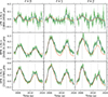 |
Fig. C.1. Temporal evolution of the averaged but not smoothed GOLF frequency shifts (dark green lines). Errors are shown as light green regions. As a reference, the dark blue line represents the smoothed frequency shifts as shown in Fig. 2. Orange and vertical grey lines have the same meaning as in Fig. 2. |
Appendix D: Results for BiSON and GONG
The main differences between the instruments are summarised as follows (see Figs. D.1 and D.2):
-
The GONG LFB of ⟨δνℓ = 0⟩ shows a clear QBO pattern that is not seen in the Sun-as-a-star instruments. Moreover, the filtered frequency ⟨δνℓ = 0⟩ follows perfectly F10.7.
-
The BiSON LFB of ⟨δνℓ = 0⟩ has the same behaviour as GOLF with an even faster rising phase of cycle 24 and a maximum earlier than in F10.7.
-
The BiSON and GONG LFBs of ⟨δνℓ = 1⟩ show similar or slightly higher amplitudes of the maximum of cycle 24 compared to cycle 23.
-
The GONG LFB of ⟨δνℓ = 2⟩ has a very low signal-to-noise ratio. As a consequence, the scaled F10.7 appears nearly flat.
-
The BiSON and GONG MFBs of ⟨δνℓ = 1⟩ do not show any excess in cycle 24 near the maximum.
Although we note differences between the instruments, we favour GOLF results as the duty cycle of the subseries are in most cases above 95% while in GONG these vary between 78% to 92% and in BiSON these are often below 65%.
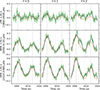 |
Fig. D.1. Temporal evolution of averaged but not smoothed BiSON frequency shifts (dark green lines) with errors represented by the light green regions. Same legend as in Fig. C.1. |
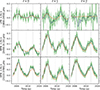 |
Fig. D.2. Temporal evolution of averaged but not smoothed GONG frequency shifts (dark green lines) with errors represented by the light green regions. The signal-to-noise ratio of ℓ=2 modes in the LFB is too low and the results are not reliable. Same legend as in Fig. C.1. |
All Tables
GOLF ⟨δν⟩ for modes ℓ = 0, 1, and 2 for the three frequency bands, LFB, MFB, and HFB.
BiSON ⟨δν⟩ for modes ℓ = 0, 1, and 2 for the three frequency bands, LFB, MFB, and HFB.
GONG ⟨δν⟩ for modes ℓ = 0, 1, and 2 for the three frequency bands, LFB, MFB, and HFB.
All Figures
|
Fig. 1. Integrated sensitivity, ⟨𝒦⟩, as a function of the relative radius for the LFB, MFB, and HFB (top, middle, and bottom panels, respectively) from the BS05 model in Bahcall & Serenelli (2005). Vertical dotted lines indicate the depth of the sensitivity kernels for ℓ = 0 modes. |
| In the text | |
|
Fig. 2. Temporal evolution of the averaged and smoothed GOLF frequency shifts (⟨δν⟩, dark blue lines) of ℓ = 0, 1, and 2 modes (left, central, and right panels respectively). The top, middle, and bottom rows correspond to the three frequency bands considered in the analysis: 1800–2450 (LFB), 2450–3110 (MFB), and 3110–3790 μHz (HFB), respectively. Light blue regions represent the errors in ⟨δν⟩. Orange lines depict the scaled smoothed F10.7 magnetic proxy. Vertical dashed and dot-dashed lines depict the maxima of cycles 23 and 24 and the minimum in between. The horizontal blue arrow indicates the change in sensitivity from the pole to the equator, and the vertical green arrow depicts the maximum sensitivity to the depth of the subsurface layers. |
| In the text | |
|
Fig. C.1. Temporal evolution of the averaged but not smoothed GOLF frequency shifts (dark green lines). Errors are shown as light green regions. As a reference, the dark blue line represents the smoothed frequency shifts as shown in Fig. 2. Orange and vertical grey lines have the same meaning as in Fig. 2. |
| In the text | |
|
Fig. D.1. Temporal evolution of averaged but not smoothed BiSON frequency shifts (dark green lines) with errors represented by the light green regions. Same legend as in Fig. C.1. |
| In the text | |
|
Fig. D.2. Temporal evolution of averaged but not smoothed GONG frequency shifts (dark green lines) with errors represented by the light green regions. The signal-to-noise ratio of ℓ=2 modes in the LFB is too low and the results are not reliable. Same legend as in Fig. C.1. |
| In the text | |
Current usage metrics show cumulative count of Article Views (full-text article views including HTML views, PDF and ePub downloads, according to the available data) and Abstracts Views on Vision4Press platform.
Data correspond to usage on the plateform after 2015. The current usage metrics is available 48-96 hours after online publication and is updated daily on week days.
Initial download of the metrics may take a while.