| Issue |
A&A
Volume 658, February 2022
|
|
|---|---|---|
| Article Number | A27 | |
| Number of page(s) | 21 | |
| Section | The Sun and the Heliosphere | |
| DOI | https://doi.org/10.1051/0004-6361/202141496 | |
| Published online | 27 January 2022 | |
No swan song for Sun-as-a-star helioseismology: Performances of the Solar-SONG prototype for individual mode characterisation
1
AIM, CEA, CNRS, Université Paris-Saclay, Université de Paris, Sorbonne Paris Cité, 91191 Gif-sur-Yvette, France
e-mail: This email address is being protected from spambots. You need JavaScript enabled to view it.
2
Instituto de Astrofísica de Canarias, 38205 La Laguna, Tenerife, Spain
3
Departamento de Astrofísica, Universidad de La Laguna (ULL), 38206 La Laguna, Tenerife, Spain
4
Stellar Astrophysics Centre, Aarhus University, 8000 Aarhus C, Denmark
Received:
8
June
2021
Accepted:
21
October
2021
Abstract
The GOLF instrument on board SoHO has been in operation for almost 25 years, but the ageing of the instrument has now strongly affected its performance, especially in the low-frequency pressure-mode (p-mode) region. At the end of the SoHO mission, the ground-based network BiSON will remain the only facility able to perform Sun-integrated helioseismic observations. Therefore, we want to assess the helioseismic performances of an échelle spectrograph such as SONG. The high precision of such an instrument and the quality of the data acquired for asteroseismic purposes call for an evaluation of the instrument’s ability to perform global radial-velocity measurements of the solar disk. Data acquired during the Solar-SONG 2018 observation campaign at the Teide Observatory are used to study mid- and low-frequency p modes. A Solar-SONG time series of 30 days in duration is reduced with a combination of the traditional IDL iSONG pipeline and a new Python pipeline described in this paper. A mode fitting method built around a Bayesian approach is then performed on the Solar-SONG and contemporaneous GOLF, BiSON, and HMI data. For this contemporaneous time series, Solar-SONG is able to characterise p modes at a lower frequency than BiSON or GOLF (1750 μHz versus 1946 and 2157 μHz, respectively), while for HMI it is possible to characterise a mode at 1686 μHz. The decrease in GOLF sensitivity is then evaluated through the evolution of its low-frequency p-mode characterisation abilities over the years: a set of 30-day-long GOLF time series, considered at the same period of the year from 1996 to 2017, is analysed. We show that it is more difficult to accurately characterise p modes in the range 1680 to 2160 μHz when considering the most recent time series. By comparing the global power level of different frequency regions, we also observe that the Solar-SONG noise level in the 1000 to 1500 μHz region is lower than for any GOLF subseries considered in this work. While the global p-mode power-level ratio is larger for GOLF during the first years of the mission, this ratio decreases over the years and is bested by Solar-SONG for every time series after 2000. All these observations strongly suggest that efforts should be made towards deploying more Solar-SONG nodes in order to acquire longer time series with better duty cycles.
Key words: Sun: helioseismology / methods: data analysis
© S. N. Breton et al. 2022
 Open Access article, published by EDP Sciences, under the terms of the Creative Commons Attribution License (http://creativecommons.org/licenses/by/4.0), which permits unrestricted use, distribution, and reproduction in any medium, provided the original work is properly cited.
1. Introduction
The first detection of oscillations in the Sun (Leighton et al. 1962; Noyes & Leighton 1963) was possibly the event that forever changed the horizon for the study of the dynamics of stellar interiors. A few years later, Ulrich (1970) and Leibacher & Stein (1971) explained those oscillations in terms of global resonant modes.
The identification of high-degree modal structure in the observed five-minute oscillations (Deubner 1975), the detections of the 160-min oscillation by Brookes et al. (1976) and Severnyi et al. (1976), identified as a possible solar internal gravity mode (g mode), and claimed oscillations in the solar diameter (Hill & Stebbins 1975) led Christensen-Dalsgaard & Gough (1976) to point out that such observations would open the way to obtaining precise inference regarding the deep interior of the Sun. The helioseismic era really began with Sun-as-a-star observations of low-degree pressure modes (p modes) by Claverie et al. (1979) and Grec et al. (1980). Several space missions, namely the Microvariability and Oscillations of STars (MOST) mission (Matthews et al. 2000), the Convection, Rotation and planetary Transit (CoRoT) satellite (Auvergne et al. 2009), the Kepler/K2 mission (Borucki et al. 2011; Howell et al. 2014), and the Transiting Exoplanet Survey Satellite (TESS, Ricker et al. 2015) opened the path for asteroseismology. Indeed, over the past two decades, asteroseismology has probed the deep layers of what now constitutes a very large number of solar-like stars (e.g., García & Ballot 2019). Moreover, solar-like oscillations observed in red giants have allowed us to derive their core rotation rate (Beck et al. 2011; Bedding et al. 2011; Mosser et al. 2011), and the resulting inferences disrupted the landscape of what was commonly accepted in stellar evolution models concerning angular momentum transport. Combined with previous results obtained with solar data, these observations have been puzzling theoreticians over the last decade (see e.g., Mathis 2013; Aerts et al. 2019, and references therein). One of the keys to the enigma resides in the deep-interior dynamics of main-sequence stars. It will be possible to set precise constraints on the core rotation rate of low-mass stars only through the detection of individual g modes in those stars. Since the first days of helioseismology, the Sun has always remained the most obvious candidate for observing g modes in a main-sequence star with solar-like pulsations (Appourchaux & Pallé 2013). Indeed, the fact that we are now able to probe the core dynamics of stars located hundreds of light years away from the Earth while being kept in the dark concerning our own star is incredibly frustrating.
Large efforts were undertaken in order to characterise solar oscillations with high precision. In 1976, Mark-I, the first node of what would become the Birmingham Solar Oscillations Network (BiSON, Chaplin et al. 1996; Davies et al. 2014; Hale et al. 2016) was deployed in Tenerife at the Teide Observatory. The International Research on the Interior of the Sun (IRIS) network (Salabert et al. 2003) operated from 1989 to 1999, and the Global Oscillations Network Group (GONG, Harvey et al. 1996) began operating in 1996. However, the culminating event of the golden era of helioseismology was without doubt the launch of the Solar Heliospheric Observatory (SoHO, Domingo et al. 1995). Bringing to space three instruments dedicated to probing the solar interior, the Global Oscillations at Low Frequency (GOLF) instrument (Gabriel et al. 1995), the Variability of solar IRradiance and Gravity Oscillations (VIRGO) instrument (Fröhlich et al. 1995), and the Solar Oscillations Investigation’s Michelson Doppler Imager (SOI/MDI) instrument (Scherrer et al. 1995), SoHO was thought to encompass all the tools needed to unravel the last mysteries hidden by the core of our star. More recently, the Solar Dynamics Observatory (SDO, Pesnell et al. 2012) was launched, including the successor to SOI/MDI, the Helioseismic Magnetic Imager (HMI) instrument (Scherrer et al. 2012).
At the time when SoHO was launched, GOLF was expected to deliver an unambiguous detection of g modes. With its sodium cell and its two photomultipliers, GOLF was designed to perform differential intensity measurements over both wings of the sodium solar doublet. Those intensity measurements allow for an extremely precise radial-velocity (RV) measurement of the upper layers of the Sun. Over the years, several individual g-mode candidates were reported (Gabriel et al. 2002; Turck-Chièze et al. 2004; García et al. 2011), and a global g-mode pattern was identified with a 99.49% confidence level (García et al. 2007). The recent claim of a g-mode detection with GOLF (Fossat et al. 2017) was reviewed by several groups who could not reproduce it and have raised serious doubts about the validity of the methodology (Schunker et al. 2018; Appourchaux & Corbard 2019; Scherrer & Gough 2019).
The Stellar Observations Network Group (SONG, Grundahl et al. 2007) initiative was conceived with the objective to install an asteroseismology-dedicated terrestrial network with several operating nodes in order to maximise the observational duty cycle. Stellar observations are performed by a robotic telescope, the light being fed to a high-resolution échelle spectrograph. The acquired spectra are then reduced to obtain high-precision RV measurements. The prototype and first node, coupled with the one-metre Hertzsprung telescope, was built at the Teide Observatory and began operation in 2014 (Andersen et al. 2016). In June 2012, as the installation of the telescope was delayed, an optical fibre mounted on a solar tracker was installed to feed solar light to the spectrograph during the day (Pallé et al. 2013). This operation represented the first light of the Solar-SONG initiative. The approach is aimed at exploiting the fact that the convective noise is expected to be partially de-correlated at different wavelengths while the p-mode signal remains coherent, as highlighted in a short test run with the GOLF New Generation (GOLF-NG) prototype (Turck-Chièze et al. 2008; Salabert et al. 2009). Independently from the Solar-SONG initiative, Sun-as-a-star observations were performed with the High Accuracy Radial velocity Planet Searcher for the Northern hemisphere (HARPS-N) spectrograph (Dumusque et al. 2015, 2021). Their purpose is to increase the precision of RV measurements by characterising and removing the stellar noise injected in the RV signal using a longer observational cadence, which is not suited for p-mode observation.
Exploiting the outcomes of the 2012 observation campaign, the power spectrum of one week of Solar-SONG observations was compared with contemporaneous GOLF and Mark-I spectra. The power in the 6000 to 8000 μHz region, dominated by photon noise, was 2.5 and 4.4 times lower than in Mark-I and GOLF, respectively. A daily low-cadence follow-up has been carried out since 2017. During the 2018 summer, a high-cadence (3.5 s) campaign of 57 days was carried out in order to evaluate the helioseismic performance of the instrument. First results of this campaign were presented in Fredslund Andersen et al. (2019a).
The potential of an échelle spectrograph such as Solar-SONG to explore the low-frequency regions of the solar power spectrum can be estimated by considering the instrument’s ability to detect low-frequency p modes. The purpose of this work is to complete and extend the previous analyses by assessing Solar-SONG performances in mid- and low-frequency p-mode ranges, using the GOLF observations, as well as BiSON and HMI observations, to evaluate the Solar-SONG capabilities.
The layout of the paper is as follows. Section 2 presents the solar time series that were used for this work. We also give some details about the Solar-SONG data reduction method. In Sect. 3, the peak-bagging of the power spectral density (PSD) obtained from the time series is described. We use the peak-bagging results to compare GOLF and Solar-SONG performances in Sect. 4. Those results and the potential of Solar-SONG are discussed in Sect. 5. For a comparison, a detailed analysis of BiSON and HMI data is included in Appendix B.
2. Data acquisition and reduction
A Solar-SONG high-cadence observation campaign took place between 27 May and 22 July, 2018. Observations were carried out in a fully automatic way and the scheduling was handled by an automation software (“the Conductor”, described in Fredslund Andersen et al. 2019b). In the work presented here, we consider only 30 days of observations, spanning 3 June to 2 July, the interval of time with the best set of consecutive days leading to a 47% duty cycle. This time range yields a good balance between spectral resolution and windowing effects due to the low duty cycle.
2.1. GOLF data reduction
Due to a loss in the counting rates measured by the photomultipliers resulting from normal ageing, the GOLF mean noise level has been increasing over the years (García et al. 2005; Appourchaux et al. 2018) in the high- and medium-frequency regions. Above 4 mHz and around 1 mHz, the photon noise power contribution dominates the PSD. We wanted to compare Solar-SONG performances not only to what GOLF performances are now, but also to what they used to be. We therefore selected 22 time series of the same length and all at similar epochs of the year in order to ensure that in each SoHO position on its orbit is comparable to what it was during the summer of 2018.
We used GOLF time series calibrated using the method described in García et al. (2005). GOLF measurements were obtained using the instrument’s own time reference and not the SoHO main on-board time reference. However, on several occasions the GOLF clock experienced unexpected events that resulted in time lags (e.g. Appourchaux et al. 2018). VIRGO is synchronised on SoHO’s main on-board clock. It was used as a reference to cross-correlate GOLF measurements and correct the timing issue of the GOLF data.
2.2. Solar-SONG data reduction
In high-cadence mode, the SONG spectrograph acquires a spectrum approximately every 3.5 s, with an exposure time below one second. The acquired spectrum covers 4400 to 6900 Å, with a pixel scale of 0.022 Å, over 51 orders. However, for solar observations, we used an iodine cell to provide precise wavelength calibration; hence for those observations only 24 orders were used, covering the 4994 to 6208 Å range where the iodine cell imprint is present. The IDL iSONG (Corsaro et al. 2012; Antoci et al. 2013) was used to compute the RVs for the solar data. The method that has been developed over the last few decades consists in dividing each order of the spectrum into so-called chunks and computing an RV for each of those chunks (see e.g., Butler et al. 1996). Twenty-two chunks per order were used for Solar-SONG spectra. For each spectrum, iSONG produces data outputs denoted as cubes. These cubes are built as 24 × 22 × 27 arrays. Indeed, 27 parameters are related to each chunk; these include the identifiers of the chunk (given by the order number and the rank of the chunk in the order), the computed RV, the photon flux level, and the observation time.
The iSONG pipeline is able to carry out the data processing and produces an integrated RV over the chunks, but we introduce in this paper a complementary code as an open source Python module called songlib, which is part of the apollinaire1 helio- and asteroseismic library (see Breton et al. in prep. and Appendix C). The new code is dedicated to obtaining the integrated RV starting from the iSONG cubes. It has the advantage of extending the original iSONG abilities by being able to reduce unequally sampled SONG data (with one spectrum acquired every ∼3.5 s) into regularly sampled velocity measurements. For this work, we produced data sampled at 20 s.
Starting from the cube output provided by the iSONG pipeline, each day of observation was then reduced individually. The first step was to integrate the chunk-relative RV to get a one-dimensional RV vector. Weights were attributed to each chunk by considering
 (1)
(1)
where σij is the robust standard deviation of the RV measurements of the jth chunk of the ith order. The robust standard deviation, σ, was computed from the median absolute deviation (MAD) as follows:
 (2)
(2)
where Φ−1 is the normal inverse cumulative distribution function evaluated at probability 3/42. If σij > 1 km s−1 or σij < 3 m s−1, the corresponding weight was set to 0. We verified that we obtained the same results with songlib and iSONG. Using the σij, the one-dimensional RV vector was computed as the weighted average of the 528 RV vectors. Considering the rms of the point-to-point difference of these daily time series (that is the difference between two consecutive measurements), we computed a proxy u for the spectrograph single-point precision (that is the typical RV uncertainty related to the acquisition of a single spectrum). The proxy was taken as the mean of the obtained rms values
 (3)
(3)
where vi and vi + 1 are consecutive RV measurements; we get 0.88 ± 0.13 m s−1.
The second step was to correct and re-sample this vector. In order to have RV measurements regularly sampled, so-called boxes of 20 seconds were computed. According to its timestamp, each cube was attributed to a box. The mean RV inside each box was computed. Values beyond three standard deviations were considered as outliers and removed. The same process was repeated with the remaining values, this time considering a two-standard-deviation threshold. To get rid of measurements that would be inconsistent with a longer trend, some outliers were again removed by considering means over a neighbourhood of 50 boxes (1000 s). Values were again removed in two steps, the first time if they were outside of eight standard deviations, the second time if they were outside six standard deviations. The RV inside each box was computed as the mean of the remaining cubes values.
The ephemeris velocity (including a barycentric correction), obtained from the IMCCE Solar system portal3, was finally subtracted from each box measurement. The Julian time noon velocity value was also subtracted from every measurement so that the residual velocity after the ephemeris correction is zero at noon (see Fig. 1).
 |
Fig. 1. Velocity residual showing the remaining trend before application of the FIR filter on the seventh day of the considered Solar-SONG time series (10 July 2018). |
The last step consists in high-pass filtering and some final corrections. During the observation campaign, the alto-azimuthal solar tracker was set to follow a pre-computed solar ephemeris without any servo correction. This introduced low-frequency daily fluctuations in the RV measurements, especially around the time of the solar meridian crossing. To filter out the harmonics that these fluctuations introduce in the spectrum below 800 μHz, we used a finite impulse response (FIR) filter. The transfer function of the FIR filter is represented in Fig. 2. The time series were extensively visually inspected and time intervals with brutal drops of absolute values of the RV measurements, clearly related to clouds obscuring the instrument line-of-sight, were set to zero at this stage4. Considering the mean photon flux level, measurements below a threshold of 12 000 analog-to-digital units (ADU) were also set to zero. We finally computed the RV mean values over the entire day. Radial velocity values beyond 3.5 standard deviation were removed. The daily RV mean was then computed again, and values beyond three standard deviations were removed.
 |
Fig. 2. Modulus of the transfer function H of the FIR filter applied to the Solar-SONG time series. |
Figure 3 shows the GOLF and Solar-SONG time series from 3 June to 2 July and the corresponding PSDs. For the sake of clarity, in the rest of the manuscript, we only compare Solar-SONG with GOLF. The analysis and comparisons done with BiSON and HMI are given in Appendix B. The results obtained with these last two instruments are qualitatively the same as with GOLF. The main difference found is between HMI and the disk-integrated instruments. The p-mode power level observed with HMI is lower than the others, which is a natural consequence of integrating the power to mimic full-disk Sun-as-a-star observations. Figure 4 shows the 1500–2500 μHz and 4000–5000 μHz regions of the PSD. The time series have been restricted to one hour and a half in Fig. 5 in order to highlight the presence of the five-minute oscillations in the signal. Figure 6 presents the same panels as in Fig. 3 but with the observational window of Solar-SONG data applied to GOLF time series. Due to the convolution by the observational window, the power of the p-mode peaks is redistributed between the main peak and the side lobes. The 800 μHz cut of the Solar-SONG time series FIR filter is visible. The comparison of the PSDs in Fig. 6 also clearly shows that the Solar-SONG mean noise level below 2000 μHz and above 6000 μHz is lower than the one in GOLF. The GOLF excess of power at the high-end frequency range of the p modes is explained by the chromospheric contribution in the sodium lines used by GOLF (Jiménez-Reyes et al. 2007).
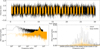 |
Fig. 3. Top panel: complete Solar-SONG (orange) and GOLF (black) time series from 3 June to 2 July 2018. Bottom left: corresponding PSDs. Bottom right: zoomed-in view of the p-mode region. |
 |
Fig. 4. GOLF (black) and Solar-SONG PSDs in the 1500–2500 μHz (top) and 4000–5000 μHz (bottom) regions. The blue line marks the n = 16, ℓ = 0 mode, which was fitted in the Solar-SONG PSD but not in the GOLF PSD. |
 |
Fig. 5. One hour and a half of the Solar-SONG (orange) and GOLF (black) RV time series. The Solar-SONG time series is sampled at 20s and the GOLF time series is sampled at 60s. |
 |
Fig. 6. Top panel: solar-SONG (orange) and GOLF (black) time series from 3 June to 2 July 2018, as in Fig. 3 but with an observational window identical that of Solar-SONG applied to the GOLF time series. Bottom left: corresponding PSDs. Bottom right: zoomed-in view of the p-mode region. |
3. Peak-bagging method
Woodard (1984) showed that the PSD follows a χ2 law with two degrees of freedom. Assuming that the frequency bins are independent of each other, the corresponding likelihood function is given by
![Mathematical equation: $$ \begin{aligned} \mathcal{L} (\boldsymbol{S_x}, \theta ) = \prod \limits _{i=1}^{k} \frac{1}{S(\nu _i, \theta )} \exp \left[ - \frac{S_{x_i}}{S(\nu _i, \theta )} \right] \;, \end{aligned} $$](/articles/aa/full_html/2022/02/aa41496-21/aa41496-21-eq4.gif) (4)
(4)
where S denotes the limit spectrum parametrised by a set θ of parameters and Sx is the observed spectrum evaluated at a given set of k frequency bins νi.
3.1. MCMC procedure
Fits were processed using a Bayesian approach through the use of Markov chains Monte Carlo (MCMCs, Sokal 1997; Liu 2009; Goodman & Weare 2010). The MCMCs properties were exploited to evaluate the shape of the posterior probability distribution of our model, using
 (5)
(5)
where p(Sx|θ) is the likelihood ℒ(Sx, θ), p(θ) the prior probability and p(Sx) a normalisation factor. In practice, only the numerator p(Sx|θ)p(θ) of the posterior probability distribution is sampled by the MCMC. In this work, all priors p(θ) have been taken as uniform distributions.
The MCMCs are sampled with the emcee5 (Foreman-Mackey 2016) implementation through the apollinaire6 (Breton et al., in prep.) peak-bagging library, which has been designed to perform analysis of both astero- and helioseismic PSDs, from stellar background profile characterisation to individual p-mode characterisation. In this work, in order to ensure their convergence, MCMCs have been sampled considering 500 walkers and 2000 iterations, with the 200 first iterations being discarded as burned-in to avoid biasing the sampled distribution. Consequently, each sampled MCMC is composed of 900 000 points after the discarding step. The uncertainties σ+ and σ− over each parameter were computed considering the 16th and 84th percentiles of the sampled distribution (which approximates the standard deviation in the case of a Gaussian distribution).
Our fitting strategy is the following. First, a global background model was adjusted to the PSD. In the second step, the PSD was divided by this background model to obtain a spectrum with a S/N scale (the so-called signal-to-noise spectrum) that we used to fit the p modes. Solar-oscillation modes can be modelled as randomly excited and damped harmonic oscillators (Goldreich & Keeley 1977; Goldreich & Kumar 1988). Therefore modes were fitted using a Lorentzian profile, by odd (ℓ = {1, 3}) and even (ℓ = {0, 2}) pairs; that is, for each pair of modes, we performed the fit considering a segment of the spectrum that contains only those modes. The Lorentzian profile equation is given by
 (6)
(6)
where νn, ℓ is the central mode frequency, Hn, ℓ the mode height, and Γn, ℓ the mode width. Due to the low resolution of the spectrum, we did not include splittings or asymmetries in our model. We also did include a flat background parameter, b, to take into account any residual local background contribution in the fitted window. For a given pair, our p-mode model Mn(ν) is therefore described by the following equations for even and odd pairs, respectively:
 (7)
(7)
Following Toutain & Appourchaux (1994), we fitted the natural logarithm of the height and width parameters. Hence, for each pair of modes, we fitted seven parameters: {νn, 0, log Hn, 0, logΓn, 0, νn − 1, 2, log Hn − 1, 2, logΓn − 1, 2, b} for even pairs and {νn, 1, log Hn, 1, logΓn, 1, νn − 1, 3, log Hn − 1, 3, logΓn − 1, 3, b} for odd pairs.
The background for the GOLF spectrum was fitted considering the sum of one Harvey profile (Harvey 1985) and a high-frequency noise parameter, P, according to the following equation:
 (8)
(8)
with A the amplitude, νc the characteristic frequency and γ a power exponent. The four parameters that we fitted are therefore A, νc, γ and P. Since the Solar-SONG time series were filtered with a high-pass filter, set to an 800-μHz cutoff frequency, we did not fit any background on the spectrum and, in order to estimate the signal-to-noise spectrum, we only divided the PSD by the mean value of the high-frequency noise (above 8 mHz).
In this work, each fitted MCMC was double-checked using the corresponding corner plots. Fits for which we did not learn anything from the priors were rejected, that is, fits where the marginalisation over each parameter of the sampled posterior probability distribution still has a uniform distribution shape. After this first step, for each fitted mode we computed a proxy of the natural logarithm of the Bayes factor, lnK, related to the rejection of the null hypothesis, H0 (Kass & Raftery 1995; Davies et al. 2016). In our case, the H0 null hypothesis is the absence of mode. For each fitted mode, we selected a given number, N, of sets of parameters among the values explored by the MCMC sampling. Those sets of parameters were selected by regularly thinning the MCMC in order to conserve the same parameter distribution in the thinned chain. For each set of parameters, the corresponding model likelihood, which was computed with a spectrum model including modes, was compared to the H0 likelihood (which was computed with a spectrum model without modes). Defining NH1 as the number of times the model likelihood is greater than the H0 likelihood, we have
 (9)
(9)
The main interest of the thinning step is to save computing time. In the work presented here, we thinned the MCMC from 900 000 to 9000 sets of parameters. The interpretation of the lnK is given in Table 1.
Interpretation of the lnK values.
3.2. Accounting for the observational windows
Since the Solar-SONG project is still a single-site ground-based instrument, its observational duty cycle is constrained by the day-night cycle. The consequence of the gaps in the time series is the convolution of the PSD by the Fourier transform of the window function (e.g. Salabert et al. 2002, 2004; García 2015). Therefore the PSD does not follow a χ2 with two degrees of freedom statistics, as the bins in the PSD are no longer independent of each other.
However, as mentioned by Gabriel (1994), the formulation of the likelihood that takes into account time series with gaps Appourchaux et al. (1998) is impracticable to use. As a consequence, the χ2 likelihood has to be used as a good approximation.
In order to take into account the effect of the window function in the PSD, we used an ad hoc correction to our model. First, we defined the observational window vector W as a boolean vector of the same length as the actual time series. Considering a given time stamp, the value of W is 1 if the RV value at this time stamp is non-zero and 0 otherwise. The Fourier transform of this window function,  , was then computed (see Fig. 7). The peaks above 1% of the height of the zero-frequency peak in
  were selected in order to modify Eq. (7) as follows:
![Mathematical equation: $$ \begin{aligned} M_n (\nu )&= \sum _k \bigg [ L_{n,0} (\nu , \nu _{n,0}+\delta \nu _k, a_k H_{n,0}, \Gamma _{n,0}) + \\&L_{n-1,2} (\nu , \nu _{n-1,2}+\delta \nu _k, a_k H_{n-1,2}, \Gamma _{n-1,2}) \bigg ] + b \;, \end{aligned} $$](/articles/aa/full_html/2022/02/aa41496-21/aa41496-21-eq12.gif) (10)
(10)
![Mathematical equation: $$ \begin{aligned} M_n (\nu )&= \sum _k \bigg [ L_{n,1} (\nu , \nu _{n,1}+\delta \nu _k, a_k H_{n,1}, \Gamma _{n,1}) + \nonumber \\&L_{n-1,3} (\nu , \nu _{n-1,3}+\delta \nu _k, a_k H_{n-1,3}, \Gamma _{n-1,3}) \bigg ] + b \;, \end{aligned} $$](/articles/aa/full_html/2022/02/aa41496-21/aa41496-21-eq13.gif) (11)
(11)
 |
Fig. 7. Power spectrum |

where δνk is the frequency of the kth selected peak in  and ak is the ratio between the height of the kth selected peak in
  and the sum of the heights of all selected peaks.
The comparison of the structure of the n = 21 even pair in GOLF data, with and without the Solar-SONG-like observational window, is shown in Fig. 8. The method presented above enables the mode profile to be accurately modelled when the observational window has daily gaps. It is also interesting to note that one of the ℓ = 0 side-lobe power excesses lies very close to the ℓ = 2 central frequency, and reciprocally for one of the ℓ = 2 side lobes.
 |
Fig. 8. Sections of power spectra for the GOLF time series (top) and the same GOLF time series truncated by the Solar-SONG observational window (bottom), centred around the n = 21 modes for the even pair (in black). The profiles corresponding to the fits are shown in red. |
4. Solar-SONG compared to GOLF
Considering the 30-day contemporaneous series, we are able to fit modes in the Solar-SONG spectrum at lower frequencies than in GOLF (even when considering the GOLF time series with full duty cycle). Indeed, the lowest-frequency fitted Solar-SONG mode is n = 11, ℓ = 1 at 1749.67 ± 1.36 μHz, while for GOLF it is n = 14, ℓ = 1 at 2156.57 ± 0.86 μHz. All the fitted frequencies are superimposed onto the échelle diagrams shown in Fig. 9. The side lobes of the ℓ = 0 and ℓ = 1 modes appear clearly in the middle and bottom panel. It should be stressed that several ℓ = 3 frequencies could not be fitted when applying the Solar-SONG-like window to GOLF, although those modes were successfully fitted in the real GOLF spectrum and in the Solar-SONG spectrum. Figures 10 and 11 show our estimates of the fitted modes height, H, and width, Γ, as a function of frequency. At high frequency, as already visible in Fig. 6, the height of the modes observed by GOLF are larger due to the chromospheric contribution to the solar sodium doublet. Most of the width values are in agreement within the error bars, except for ℓ = 1 modes, where Solar-SONG-observed widths seem overestimated below 3 mHz, although the fitted values remain compatible within the error bars with what we have measured with GOLF.
 |
Fig. 9. Échelle diagram for GOLF (top), GOLF with a Solar-SONG-like observational window (middle), and Solar-SONG (bottom). Fitted mode frequencies are represented in black. |
 |
Fig. 10. Heights, H, of the fitted mode for GOLF (black), GOLF with the Solar-SONG window (grey) and Solar-SONG (orange) spectra. The horizontal position of the markers has been slightly shifted for visualisation convenience. |
Another interesting aspect of the comparison between the two instruments is the inability of the code to fit the n = 16, ℓ = 0 mode in the GOLF spectrum; this same mode is well characterised using Solar-SONG. In the top panel of Fig. 4, it appears that during the time of observation, this mode was less excited than its ℓ = 0 and ℓ = 1 neighbours, making it more difficult to detect with both instruments. The mode structure is also difficult to distinguish from the surrounding noise in the GOLF PSD, while the S/N appears to be higher in the Solar-SONG PSD. This can be explained by both the higher level of noise in the GOLF PSD and the different spatial sensitivity of GOLF in its single-wing configuration. As shown by García et al. (1998) and Henney (1999), the sensitivity of GOLF depends on the observation wing (blue or red) and on the time of the year (due to the non-zero orbital velocity). Thus, excited modes can have different amplitudes in GOLF than in other instruments with a homogeneous response window.
We include in the appendix (see Tables A.1–A.3) all the fitted mode frequencies, heights, and widths, as well as their uncertainties and the corresponding value of lnK. We note that the smallest frequency uncertainty estimates are comparable to the spectral resolution of 0.39 μHz
Based on the total power in the 1000–1500 μHz region of the GOLF data, Appourchaux et al. (2018) showed evidence of an increase in the noise at low frequency over the past two decades, noise that is due to the instrument photon noise and the contribution of solar convection to the RV signal. This increase is most likely due to the ageing of the two photomultipliers, of the entrance window, and of the interference filter, as already pointed out by García et al. (2005) based on the increase in instrumental photon noise between 1996 and 2004. It is straightforward to verify, considering the 2018 observing campaign, that the mean power density in the 1000–1500 μHz region is in favour of Solar-SONG. This value is 29.1 m2 s−2 Hz−1 versus 104 m2 s−2 Hz−1 for GOLF. We note that the same comparison in the 5000–6000 μHz region yields 14 m2 s−2 Hz−1 for Solar-SONG and 103 m2 s−2 Hz−1 for GOLF.
The top panel of Fig. 12 shows the mean power density in the 1000–1500 μHz region for each 30-day GOLF time series considered in this work (see Sect. 2.1). The middle panel shows the ratio between the mean power density in the 2000–3500 μHz region and the mean power density in the 1000–1500 μHz region. The bottom panel shows the same ratio for the 1700–2200 μHz region, which is the lowest-frequency region where we were able to fit modes for Solar-SONG. In each panel, the value we obtain with the Solar-SONG time series is also represented.
 |
Fig. 12. Top: mean power density in the 1000–1500 μHz region of the considered 30-day GOLF and Solar-SONG PSDs. Middle: mean power density ratio computed as the ratio between the mean power in the 2000–3500 μHz p-mode region and the 1000–1500 μHz region. Bottom: mean power density ratio computed as the ratio between the mean power in the 1700–2200 μHz region and the 1000–1500 μHz region. The dotted yellow line represents the value obtained with Solar-SONG during the 2018 campaign (represented by the yellow dot). |
The temporal evolution of the mean power density in the 1000–1500 μHz region unveils evidence that the Solar-SONG noise level in this region is comparable to, if not smaller than what it was for GOLF in the instrument’s best years. The power decrease observed from 1996 to 1999 can probably be linked to the minimum of magnetic activity reached at this time. After this date, ignoring some yearly modulations, the mean power density in this frequency region increases continually.
Concerning the mean power density ratio between 2000 and 3500 μHz, for the 2018 time series we obtain a 9.8 ratio for Solar-SONG versus 3.6 for GOLF. However, we note that in the first years of GOLF operations, this value was much higher (13.6 in 1996). During the year 2000, it reached the Solar-SONG level and then kept on decreasing.
In the 1700–2200 μHz region, we find a maximal ratio of 1.16 for GOLF (in 2001) and 0.9 in 2018, while we have 1.3 for Solar-SONG. To help visually assess the signification of this difference in ratio, we represent in Fig. 13 the normalised PSD of the 1700–2200 μHz region for GOLF (considering the time series with a Solar-SONG-like window) and Solar-SONG. The normalisation was performed by dividing each PSD by its median value in the 1700–2200 μHz region. With this normalisation, it appears that, in this specific region, most of the p modes have a relative height that is higher in Solar-SONG than in GOLF. These elements combined with our ability to fit several modes for Solar-SONG in this frequency region therefore strongly suggest that the S/N is also in favour of Solar-SONG in this frequency range.
 |
Fig. 13. GOLF (with a Solar-SONG observational window, black) and Solar-SONG (orange) normalised PSDs between 1700 and 2200 μHz. The normalisation has been performed by dividing each PSD by its median value in the 1700–2200 μHz region. The frequencies fitted in the Solar-SONG spectrum are marked by vertical lines with a colour-coding related to the mode degree: blue, red, light blue, and pink for ℓ = 0, 1, 2, and 3, respectively. |
The second step of this GOLF yearly evolution analysis was to consider the mode orders for which, considering the 2018 GOLF series, we were not able to provide mode parameters but for which some modes were fitted considering Solar-SONG data. With Solar-SONG, we were able to fit the n = 11, ℓ = 1 mode while for GOLF we had to stop at the n = 14, ℓ = 1 mode. We therefore decided to perform our peak-bagging process for odd and even pairs of order 11 to 14 on each GOLF 30-day series. The results are summarised order by order and degree by degree in Fig. 14. The mode frequency variations are related to the magnetic solar activity (Woodard & Noyes 1985; Palle et al. 1989). Modes that are not represented in this figure could not be fitted or the uncertainty on fitted frequency was above 2 μHz. The n = 11, ℓ = 1 could not be fitted in the considered GOLF series after 2005. For this order, we were not able to fit any ℓ = 2 or ℓ = 3 modes. The only mode we were able to fit almost every time until 2018 is the n = 14, ℓ = 1. It should be recalled that for such short time series, our ability to fit a given mode is not only dependent on the instrumental S/N but also on the excitation state of the mode. This explains why for certain 30-day series, some modes could not be fitted despite GOLF instrumental noise not increasing drastically or being even lower. It should be noted that this GOLF performance analysis over time is only valid for 30-day-long time series. By considering longer GOLF time series, it is of course possible to obtain much better constraints for the mode parameters in the frequency region considered in Fig. 14 (see e.g., Salabert et al. 2015, which used 365-day long GOLF time series to probe the p-mode temporal frequency variation).
 |
Fig. 14. Fitted mode frequencies and uncertainties for yearly GOLF 30-day series (black). The uncertainties on mode frequencies fitted within the Solar-SONG spectrum are represented in orange for the purpose of comparison. The white tick signals the median value of the fitted distribution. For both instruments, only modes with an uncertainty below 2 μHz are represented. |
5. The future of Solar-SONG: Discussion and conclusion
In this work we have presented a new reduction pipeline for Solar-SONG data. We compared the contemporaneous GOLF (as well as BiSON and HMI) and Solar-SONG observations by performing a peak-bagging analysis with a Bayesian approach. On the one hand, by studying the PSD of the Solar-SONG data, we were able to identify modes at lower frequency than in the GOLF PSD. On the other hand, we evaluated the effect of the ageing of GOLF on its performance by considering the yearly mean power evolution in the 1000 to 1500 μHz region with 30-day-long series. For each considered series, the mean power density was above the mean power density obtained in 2018 with Solar-SONG. However, the GOLF global p-mode power density ratio in the 2000–3500 μHz region was above the Solar-SONG level from 1996 to 1999. This power density ratio decreased over the years. In 2018, the Solar-SONG power density ratio was almost three times higher than the GOLF power density ratio. Considering the 1700–2200 μHz region only, the Solar-SONG power density ratio appears higher than the GOLF power density ratio at any time.
We then performed another peak-bagging analysis on these series, focusing on the low-frequency p modes (below 2200 μHz) for which we were able to provide more precise mode frequencies for Solar-SONG but not for GOLF in the 2018 comparison. We were able to provide frequencies for many of these modes in the first years of SoHO’s operations. However, after 2005, the decrease in S/N reduced the number of modes we were able to fit inside each subseries.
Despite its ageing, GOLF remains an invaluable asset for helioseismology. It has been almost continuously collecting data over the last 25 years and will carry on in its mission in the years to come. However, the promising helioseismic measurements obtained during the Solar-SONG 2018 summer high-cadence run show the potential of longer observations with a better duty cycle. This second condition can only be achieved if other SONG nodes are available. Presently, a new node of the SONG network is being commissioned at the Mt. Kent Observatory in Queensland, Australia. Performing observations with both Australian and Canarian SONG nodes would allow a significant improvement in the time series duty cycle, although it would still be necessary to continue extending the SONG network in order to reach a constant duty cycle above 80%.
In order to improve the S/N of the low-frequency regions of the Solar-SONG PSD, the solar tracker used for the 2018 observation campaign should also be modified. The current Solar-SONG setup uses an azimuthal commercial mount, which is not optimal for stability in frequency regions below 800 μHz. Indeed, the daily Earth-motion RV residual that appears in Fig. 1 creates a high-amplitude harmonic pattern in the PSD if the low-frequency trend of the Solar-SONG time series has not been properly filtered out with the FIR filter. It should be noted that the servo guidance was not active during the 2018 campaign. The solar tracker followed the Sun’s motion using only a pre-computed ephemeris. However, we noticed during a short test run performed in 2019 that turning on the servo introduced additional low-frequency trends to the RV signal. In order to overcome this limitation and to extend the scientific objectives of the Solar-SONG initiative, funding was obtained for a new project, baptised Magnetrometry Unit for SOLar-SONG (MUSOL), which plans to upgrade the Solar-SONG Teide node with both an equatorial mount that will allow improved guidance and a new polarimetric unit. Indeed, the dipolar and quadrupolar components of the solar global magnetic field can only be measured by detecting the weak polarisation signal induced in some spectral lines by the Hanle effect. Long-term and continuous solar observations with this new polarimetric unit should in principle be sensitive enough to measure the dipolar component of the global solar magnetic field and its variation along the solar activity cycle (see Vieu et al. 2017).
The source code is available at https://gitlab.com/sybreton/apollinaire
See the astropy (Astropy Collaboration 2013, 2018) documentation at: https://docs.astropy.org/en/stable/api/astropy.stats.mad_std.html
Available at: https://ssp.imcce.fr/forms/visibility
The exhaustive list of corrections can be found at: https://gitlab.com/sybreton/apollinaire/-/blob/master/apollinaire/songlib/interval_nan.py
The module documentation is available at: https://emcee.readthedocs.io/en/stable
The module documentation is available at: https://apollinaire.readthedocs.io/en/latest
Available on the BiSON website at:
Available at:
Acknowledgments
The authors want to thank the anonymous referee for valuable comments that helped in improving the manuscript. This work is based on observations made at the Hertzsprung SONG telescope operated at the Spanish Observatorio del Teide on the island of Tenerife by the Aarhus and Copenhagen Universities and by the Instituto de Astrofísica de Canarias. SoHO is a mission of international collaboration between ESA and NASA. S.N.B. and R.A.G acknowledge the support from PLATO and GOLF CNES grants. Funding for Solar-SONG was provided by the Excellence ’Severo Ochoa’ programme at the IAC and the Ministry MINECO under the program AYA-2016-76378-P. Funding for the Stellar Astrophysics Centre is provided by The Danish National Research Foundation (Grant DNRF106). We would like to acknowledge the contribution of the engineers at the IAC, Felix Gracia (optical), Ezequiel Ballesteros (electronics) and the support from the day-time operator at the SolarLab, Teide Observatory, on this Solar-SONG initiative and during the campaign. We thank Dr. Kun Wang (China West Normal University) for his dedicated effort during the campaign with data handling and analysis of the observations. We also thank Thierry Appourchaux for his relevant comments during the TASOC review. The solar visibility calculations were carried out by the ephemeris calculation service of the IMCCE through its Solar System portal (https://ssp.imcce.fr). Software: Python (Van Rossum & Drake 2009), numpy (Oliphant 2006; Harris et al. 2020), pandas (Pandas development team 2020; McKinney 2010), matplotlib (Hunter 2007), emcee (Foreman-Mackey et al. 2013), scipy (Virtanen et al. 2020), corner (Foreman-Mackey 2016), astropy (Astropy Collaboration 2013, 2018). The source code used to obtain the present results can be found at gitlab.com/sybreton/apollinaire.
References
- Aerts, C., Mathis, S., & Rogers, T. M. 2019, ARA&A, 57, 35 [Google Scholar]
- Andersen, M. F., Grundahl, F., Beck, A. H., & Pallé, P. 2016, Rev. Mex. Astron. Astrofis. Conf. Ser., 48, 54 [NASA ADS] [Google Scholar]
- Antoci, V., Handler, G., Grundahl, F., et al. 2013, MNRAS, 435, 1563 [NASA ADS] [CrossRef] [Google Scholar]
- Appourchaux, T., & Corbard, T. 2019, A&A, 624, A106 [NASA ADS] [CrossRef] [EDP Sciences] [Google Scholar]
- Appourchaux, T., & Pallé, P. L. 2013, in Fifty Years of Seismology of the Sun and Stars, eds. K. Jain, S. C. Tripathy, F. Hill, J. W. Leibacher, & A. A. Pevtsov, ASP Conf. Ser., 478, 125 [NASA ADS] [Google Scholar]
- Appourchaux, T., Gizon, L., & Rabello-Soares, M. C. 1998, A&AS, 132, 107 [NASA ADS] [CrossRef] [EDP Sciences] [Google Scholar]
- Appourchaux, T., Boumier, P., Leibacher, J. W., & Corbard, T. 2018, A&A, 617, A108 [NASA ADS] [CrossRef] [EDP Sciences] [Google Scholar]
- Astropy Collaboration (Robitaille, T. P., et al.) 2013, A&A, 558, A33 [NASA ADS] [CrossRef] [EDP Sciences] [Google Scholar]
- Astropy Collaboration (Price-Whelan, A. M., et al.) 2018, AJ, 156, 123 [Google Scholar]
- Auvergne, M., Bodin, P., Boisnard, L., et al. 2009, A&A, 506, 411 [NASA ADS] [CrossRef] [EDP Sciences] [Google Scholar]
- Beck, P. G., Bedding, T. R., Mosser, B., et al. 2011, Science, 332, 205 [Google Scholar]
- Bedding, T. R., Mosser, B., Huber, D., et al. 2011, Nature, 471, 608 [Google Scholar]
- Borucki, W. J., Koch, D. G., Basri, G., et al. 2011, ApJ, 736, 19 [Google Scholar]
- Brookes, J. R., Isaak, G. R., & van der Raay, H. B. 1976, Nature, 259, 92 [Google Scholar]
- Butler, R. P., Marcy, G. W., Williams, E., et al. 1996, PASP, 108, 500 [Google Scholar]
- Chaplin, W. J., Elsworth, Y., Howe, R., et al. 1996, Sol. Phys., 168, 1 [NASA ADS] [CrossRef] [Google Scholar]
- Christensen-Dalsgaard, J., & Gough, D. O. 1976, Nature, 259, 89 [NASA ADS] [CrossRef] [Google Scholar]
- Claverie, A., Isaak, G. R., McLeod, C. P., van der Raay, H. B., & Cortes, T. R. 1979, Nature, 282, 591 [NASA ADS] [CrossRef] [Google Scholar]
- Corsaro, E., Grundahl, F., Leccia, S., et al. 2012, A&A, 537, A9 [NASA ADS] [CrossRef] [EDP Sciences] [Google Scholar]
- Davies, G. R., Chaplin, W. J., Elsworth, Y. P., & Hale, S. J. 2014, MNRAS, 441, 3009 [NASA ADS] [CrossRef] [Google Scholar]
- Davies, G. R., Silva Aguirre, V., Bedding, T. R., et al. 2016, MNRAS, 456, 2183 [Google Scholar]
- Deubner, F. L. 1975, A&A, 44, 371 [Google Scholar]
- Domingo, V., Fleck, B., & Poland, A. I. 1995, Sol. Phys., 162, 1 [Google Scholar]
- Dumusque, X., Glenday, A., Phillips, D. F., et al. 2015, ApJ, 814, L21 [Google Scholar]
- Dumusque, X., Cretignier, M., Sosnowska, D., et al. 2021, A&A, 648, A103 [NASA ADS] [CrossRef] [EDP Sciences] [Google Scholar]
- Foreman-Mackey, D. 2016, J. Open Source Softw., 1, 24 [Google Scholar]
- Foreman-Mackey, D., Hogg, D. W., Lang, D., & Goodman, J. 2013, PASP, 125, 306 [Google Scholar]
- Fossat, E., Boumier, P., Corbard, T., et al. 2017, A&A, 604, A40 [NASA ADS] [CrossRef] [EDP Sciences] [Google Scholar]
- Fredslund Andersen, M., Pallé, P., Jessen-Hansen, J., et al. 2019a, A&A, 623, L9 [NASA ADS] [CrossRef] [EDP Sciences] [Google Scholar]
- Fredslund Andersen, M., Handberg, R., Weiss, E., et al. 2019b, PASP, 131, 045003 [Google Scholar]
- Fröhlich, C., Romero, J., Roth, H., et al. 1995, Sol. Phys., 162, 101 [Google Scholar]
- Gabriel, A. H., Grec, G., Charra, J., et al. 1995, Sol. Phys., 162, 61 [Google Scholar]
- Gabriel, A. H., Baudin, F., Boumier, P., et al. 2002, A&A, 390, 1119 [NASA ADS] [CrossRef] [EDP Sciences] [Google Scholar]
- Gabriel, M. 1994, A&A, 287, 685 [NASA ADS] [Google Scholar]
- García, R. A. 2015, EAS Pub. Ser., 73, 193 [CrossRef] [EDP Sciences] [Google Scholar]
- García, R. A., & Ballot, J. 2019, Liv. Rev. Sol. Phys., 16, 4 [Google Scholar]
- García, R. A., Pallé, P. L., Turck-Chièze, S., et al. 1998, ApJ, 504, L51 [CrossRef] [Google Scholar]
- García, R. A., Turck-Chièze, S., Boumier, P., et al. 2005, A&A, 442, 385 [NASA ADS] [CrossRef] [EDP Sciences] [Google Scholar]
- García, R. A., Turck-Chièze, S., Jiménez-Reyes, S. J., et al. 2007, Science, 316, 1591 [Google Scholar]
- García, R. A., Salabert, D., Ballot, J., et al. 2011, J. Phys. Conf. Ser., 271, 012046 [CrossRef] [Google Scholar]
- Goldreich, P., & Keeley, D. A. 1977, ApJ, 212, 243 [NASA ADS] [CrossRef] [Google Scholar]
- Goldreich, P., & Kumar, P. 1988, ApJ, 326, 462 [CrossRef] [Google Scholar]
- Goodman, J., & Weare, J. 2010, Comm. Appl. Math. Comput. Sci., 5, 65 [Google Scholar]
- Grec, G., Fossat, E., & Pomerantz, M. 1980, Nature, 288, 541 [CrossRef] [Google Scholar]
- Grundahl, F., Kjeldsen, H., Christensen-Dalsgaard, J., Arentoft, T., & Frandsen, S. 2007, Commun. Asteroseismol., 150, 300 [NASA ADS] [CrossRef] [Google Scholar]
- Hale, S. J., Howe, R., Chaplin, W. J., Davies, G. R., & Elsworth, Y. P. 2016, Sol. Phys., 291, 1 [NASA ADS] [CrossRef] [Google Scholar]
- Harris, C. R., Millman, K. J., van der Walt, S. J., et al. 2020, Nature, 585, 357 [NASA ADS] [CrossRef] [Google Scholar]
- Harvey, J. 1985, in Future Missions in Solar, Heliospheric& Space Plasma Physics, eds. E. Rolfe, & B. Battrick, ESA SP, 235, 199 [NASA ADS] [Google Scholar]
- Harvey, J. W., Hill, F., Hubbard, R. P., et al. 1996, Science, 272, 1284 [Google Scholar]
- Henney, C. J. 1999, Ph.D. Thesis, University of California, Los Angeles, USA [Google Scholar]
- Hill, H. A., & Stebbins, R. T. 1975, in Seventh Texas Symposium on Relativistic Astrophysics, eds. P. G. Bergman, E. J. Fenyves, & L. Motz, 262, 472 [NASA ADS] [Google Scholar]
- Howell, S. B., Sobeck, C., Haas, M., et al. 2014, PASP, 126, 398 [Google Scholar]
- Hunter, J. D. 2007, Comput. Sci. Eng., 9, 90 [NASA ADS] [CrossRef] [Google Scholar]
- Jiménez-Reyes, S. J., Chaplin, W. J., Elsworth, Y., et al. 2007, ApJ, 654, 1135 [CrossRef] [Google Scholar]
- Kass, R. E., & Raftery, A. E. 1995, J. Am. Stat. Assoc., 90, 773 [Google Scholar]
- Larson, T. P., & Schou, J. 2015, Sol. Phys., 290, 3221 [NASA ADS] [CrossRef] [Google Scholar]
- Leibacher, J. W., & Stein, R. F. 1971, Astrophys. Lett., 7, 191 [NASA ADS] [Google Scholar]
- Leighton, R. B., Noyes, R. W., & Simon, G. W. 1962, ApJ, 135, 474 [NASA ADS] [CrossRef] [Google Scholar]
- Liu, J. 2009, Monte Carlo Strategies in Scientic Computing [Google Scholar]
- Mathis, S. 2013, in Transport Processes in Stellar Interiors, eds. M. Goupil, K. Belkacem, C. Neiner, F. Lignières, & J. J. Green, 865, 23 [Google Scholar]
- Matthews, J. M., Kuschnig, R., & Walker, G. A. H. 2000, in IAU Colloq. 176: The Impact of Large-Scale Surveys on Pulsating Star Research, eds. L. Szabados, & D. Kurtz, ASP Conf. Ser., 203, 74 [NASA ADS] [Google Scholar]
- McKinney, W. 2010, in Proceedings of the 9th Python in Science Conference, eds. S. van der Walt, & J. Millman, 56 [Google Scholar]
- Mosser, B., Barban, C., Montalbán, J., et al. 2011, A&A, 532, A86 [NASA ADS] [CrossRef] [EDP Sciences] [Google Scholar]
- Noyes, R. W., & Leighton, R. B. 1963, ApJ, 138, 631 [NASA ADS] [CrossRef] [Google Scholar]
- Oliphant, T. 2006, NumPy: A guide to NumPy (USA: Trelgol Publishing) [Google Scholar]
- Palle, P. L., Regulo, C., & Roca Cortes, T. 1989, A&A, 224, 253 [NASA ADS] [Google Scholar]
- Pallé, P. L., Grundahl, F., Triviño Hage, A., et al. 2013, J. Phys. Conf. Ser., 440, 012051 [CrossRef] [Google Scholar]
- Pandas development team 2020, Pandas-dev/pandas: Pandas [Google Scholar]
- Pesnell, W. D., Thompson, B. J., & Chamberlin, P. C. 2012, Sol. Phys., 275, 3 [Google Scholar]
- Ricker, G. R., Winn, J. N., Vanderspek, R., et al. 2015, J. Astron. Telescopes Instrum. Syst., 1, 014003 [Google Scholar]
- Salabert, D., Fossat, E., Gelly, B., et al. 2002, A&A, 390, 717 [NASA ADS] [CrossRef] [EDP Sciences] [Google Scholar]
- Salabert, D., Jiménez-Reyes, S. J., & Tomczyk, S. 2003, A&A, 408, 729 [NASA ADS] [CrossRef] [EDP Sciences] [Google Scholar]
- Salabert, D., Fossat, E., Gelly, B., et al. 2004, A&A, 413, 1135 [NASA ADS] [CrossRef] [EDP Sciences] [Google Scholar]
- Salabert, D., García, R. A., & Turck-Chièze, S. 2015, A&A, 578, A137 [NASA ADS] [CrossRef] [EDP Sciences] [Google Scholar]
- Salabert, D., Turck-Chièze, S., Barrière, J. C., et al. 2009, in Solar-Stellar Dynamos as Revealed by Helio- and Asteroseismology: GONG 2008/SOHO 21, eds. M. Dikpati, T. Arentoft, I. González Hernández, C. Lindsey, & F. Hill, ASP Conf. Ser., 416, 341 [NASA ADS] [Google Scholar]
- Scherrer, P. H., & Gough, D. O. 2019, ApJ, 877, 42 [Google Scholar]
- Scherrer, P. H., Bogart, R. S., Bush, R. I., et al. 1995, Sol. Phys., 162, 129 [Google Scholar]
- Scherrer, P. H., Schou, J., Bush, R. I., et al. 2012, Sol. Phys., 275, 207 [Google Scholar]
- Schunker, H., Schou, J., Gaulme, P., & Gizon, L. 2018, Sol. Phys., 293, 95 [Google Scholar]
- Severnyi, A. B., Kotov, V. A., & Tsap, T. T. 1976, Nature, 259, 87 [Google Scholar]
- Sokal, A. 1997, in Monte Carlo Methods in Statistical Mechanics: Foundations and New Algorithms, eds. C. DeWitt-Morette, P. Cartier, & A. Folacci (Boston, MA: Springer, US), 131 [Google Scholar]
- Toutain, T., & Appourchaux, T. 1994, A&A, 289, 649 [NASA ADS] [Google Scholar]
- Turck-Chièze, S., García, R. A., Couvidat, S., et al. 2004, ApJ, 604, 455 [Google Scholar]
- Turck-Chièze, S., Mathur, S., Ballot, J., et al. 2008, J. Phys. Conf. Ser., 118, 012044 [CrossRef] [Google Scholar]
- Ulrich, R. K. 1970, ApJ, 162, 993 [NASA ADS] [CrossRef] [Google Scholar]
- Van Rossum, G., & Drake, F. L. 2009, Python 3 Reference Manual (Scotts Valley, CA: CreateSpace) [Google Scholar]
- Vieu, T., Martínez González, M. J., Pastor Yabar, A., & Asensio Ramos, A. 2017, MNRAS, 465, 4414 [NASA ADS] [CrossRef] [Google Scholar]
- Virtanen, P., Gommers, R., Oliphant, T. E., et al. 2020, Nat. Methods, 17, 261 [Google Scholar]
- Woodard, M. F. 1984, Ph.D. Thesis, University of California, San Diego, USA [Google Scholar]
- Woodard, M. F., & Noyes, R. W. 1985, Nature, 318, 449 [NASA ADS] [CrossRef] [Google Scholar]
Appendix A: Fitting results for GOLF and Solar-SONG
The full summary of the GOLF and Solar-SONG fits performed for this work is presented in this section. Table A.1 presents the mode parameters obtained with GOLF, Table A.2 the mode parameters obtained with GOLF when applying a Solar-SONG-like window and Table A.3 the mode parameters obtained with Solar-SONG.
Parameters of the modes fitted in the GOLF spectrum.
Same as Table A.1 but for the GOLF spectrum obtained with the series multiplied by the Solar-SONG-like window.
Same as Table A.1, but for Solar-SONG spectrum.
Appendix B: Comparison with HMI and BiSON
Here, the study of the contemporaneous HMI and BiSON 30-day series (spanning from from 3 June to 2 July) is performed and compared to the Solar-SONG data similar to what was done in Sect. 3. The BiSON subseries are extracted from the January 1976 to March 2020 optimised-for-fill time series7, while the considered HMI time series is obtained from the ℓ = 0 reduction of the HMI full-disk Dopplergrams8 (Larson & Schou 2015). The duty cycle of the complete BiSON series is 63.5% while it is 100% for HMI. For each instrument we did two analyses, one with the original duty cycle and the other using the Solar-SONG observational window function (that is by simply multiplying the time series with the Solar-SONG window function). As the duty cycle of the considered BiSON time series is significantly below 90%, we used the method described in Sect. 3.2 to fit the PSD of this time series, similarly to what was done for all the time series with the Solar-SONG observational window. Table B.1 compares the mean power value in the 1000-1500 μHz region and the power ratio in the 2000-3500 μHz and 1700-2200 μHz regions as explained in Sect. 4. Figure B.1 shows the four échelle diagrams. HMI- and BiSON-fitted heights and widths are represented together with the values fitted for GOLF and Solar-SONG in Figs. B.2 and B.3, respectively. All the fitted parameters, uncertainties and the corresponding lnK are summarised in Tables B.2, B.3, B.4, and B.5, respectively.
We note that the mode heights in HMI are significantly lower than for the other instruments, which is expected as we considered only the ℓ = 0 time series. For both HMI and BiSON, the ratio between the mean power density in the 2000-3500 μHz region and the mean power density in the 1000-1500 μHz region is close to the 9.8 value obtained with Solar-SONG and well above the 3.6 value of GOLF in 2018. The ratio between the mean power density in the 1700-2200 μHz region and the mean power density in the 1000-1500 μHz region is also similar for the four instruments: 1.3, 0.9, 1.1, and 1.0 for Solar-SONG, GOLF, BiSON, and HMI, respectively. The characterisation of modes below 1700 μHz is only possible using HMI data. The n = 11, ℓ = 0 mode was properly fitted, and a frequency of 1686.73 ± 0.14 μHz was obtained.
Mean power and mean power ratios for each considered instrument.
 |
Fig. B.1. Échelle diagram for BiSON (top left), BiSON with a Solar-SONG-like observational window (top right), HMI (bottom left) and HMI with a Solar-SONG-like observational window (bottom right). Fitted modes frequencies are represented in black. |
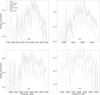 |
Fig. B.2. Heights, H, of the fitted modes for GOLF (black), GOLF with the Solar-SONG window (grey), Solar-SONG (orange), BiSON (blue), BiSON with the Solar-SONG window (light blue), HMI (green), and HMI with the Solar-SONG window (light green) spectra. The horizontal position of the markers has been slightly shifted for visualisation convenience. |
Parameters of the modes fitted in the BiSON spectrum.
Same as Table B.2 but for the BiSON spectrum obtained with the series multiplied by the Solar-SONG-like window.
Parameters of the modes fitted in the HMI spectrum.
Same as Table B.4 but for the HMI spectrum obtained with the series multiplied by the Solar-SONG-like window.
Appendix C: Solar-SONG data reduction module
The reduction process described in Sect. 2 can be performed with the songlib submodule of apollinaire. The standard_correction function has been designed to process the iSONG cube outputs. The default settings of the function arguments are the ones that have been used to obtain the data used in this paper.
All Tables
Same as Table A.1 but for the GOLF spectrum obtained with the series multiplied by the Solar-SONG-like window.
Same as Table B.2 but for the BiSON spectrum obtained with the series multiplied by the Solar-SONG-like window.
Same as Table B.4 but for the HMI spectrum obtained with the series multiplied by the Solar-SONG-like window.
All Figures
|
Fig. 1. Velocity residual showing the remaining trend before application of the FIR filter on the seventh day of the considered Solar-SONG time series (10 July 2018). |
| In the text | |
|
Fig. 2. Modulus of the transfer function H of the FIR filter applied to the Solar-SONG time series. |
| In the text | |
|
Fig. 3. Top panel: complete Solar-SONG (orange) and GOLF (black) time series from 3 June to 2 July 2018. Bottom left: corresponding PSDs. Bottom right: zoomed-in view of the p-mode region. |
| In the text | |
|
Fig. 4. GOLF (black) and Solar-SONG PSDs in the 1500–2500 μHz (top) and 4000–5000 μHz (bottom) regions. The blue line marks the n = 16, ℓ = 0 mode, which was fitted in the Solar-SONG PSD but not in the GOLF PSD. |
| In the text | |
|
Fig. 5. One hour and a half of the Solar-SONG (orange) and GOLF (black) RV time series. The Solar-SONG time series is sampled at 20s and the GOLF time series is sampled at 60s. |
| In the text | |
|
Fig. 6. Top panel: solar-SONG (orange) and GOLF (black) time series from 3 June to 2 July 2018, as in Fig. 3 but with an observational window identical that of Solar-SONG applied to the GOLF time series. Bottom left: corresponding PSDs. Bottom right: zoomed-in view of the p-mode region. |
| In the text | |
|
Fig. 7. Power spectrum |
| In the text | |
|
Fig. 8. Sections of power spectra for the GOLF time series (top) and the same GOLF time series truncated by the Solar-SONG observational window (bottom), centred around the n = 21 modes for the even pair (in black). The profiles corresponding to the fits are shown in red. |
| In the text | |
|
Fig. 9. Échelle diagram for GOLF (top), GOLF with a Solar-SONG-like observational window (middle), and Solar-SONG (bottom). Fitted mode frequencies are represented in black. |
| In the text | |
|
Fig. 10. Heights, H, of the fitted mode for GOLF (black), GOLF with the Solar-SONG window (grey) and Solar-SONG (orange) spectra. The horizontal position of the markers has been slightly shifted for visualisation convenience. |
| In the text | |
 |
Fig. 11. Same as in Fig. 10 but for mode widths, Γ. |
| In the text | |
|
Fig. 12. Top: mean power density in the 1000–1500 μHz region of the considered 30-day GOLF and Solar-SONG PSDs. Middle: mean power density ratio computed as the ratio between the mean power in the 2000–3500 μHz p-mode region and the 1000–1500 μHz region. Bottom: mean power density ratio computed as the ratio between the mean power in the 1700–2200 μHz region and the 1000–1500 μHz region. The dotted yellow line represents the value obtained with Solar-SONG during the 2018 campaign (represented by the yellow dot). |
| In the text | |
|
Fig. 13. GOLF (with a Solar-SONG observational window, black) and Solar-SONG (orange) normalised PSDs between 1700 and 2200 μHz. The normalisation has been performed by dividing each PSD by its median value in the 1700–2200 μHz region. The frequencies fitted in the Solar-SONG spectrum are marked by vertical lines with a colour-coding related to the mode degree: blue, red, light blue, and pink for ℓ = 0, 1, 2, and 3, respectively. |
| In the text | |
|
Fig. 14. Fitted mode frequencies and uncertainties for yearly GOLF 30-day series (black). The uncertainties on mode frequencies fitted within the Solar-SONG spectrum are represented in orange for the purpose of comparison. The white tick signals the median value of the fitted distribution. For both instruments, only modes with an uncertainty below 2 μHz are represented. |
| In the text | |
|
Fig. B.1. Échelle diagram for BiSON (top left), BiSON with a Solar-SONG-like observational window (top right), HMI (bottom left) and HMI with a Solar-SONG-like observational window (bottom right). Fitted modes frequencies are represented in black. |
| In the text | |
|
Fig. B.2. Heights, H, of the fitted modes for GOLF (black), GOLF with the Solar-SONG window (grey), Solar-SONG (orange), BiSON (blue), BiSON with the Solar-SONG window (light blue), HMI (green), and HMI with the Solar-SONG window (light green) spectra. The horizontal position of the markers has been slightly shifted for visualisation convenience. |
| In the text | |
 |
Fig. B.3. Same as in Fig. B.2 but for mode widths, Γ. |
| In the text | |
Current usage metrics show cumulative count of Article Views (full-text article views including HTML views, PDF and ePub downloads, according to the available data) and Abstracts Views on Vision4Press platform.
Data correspond to usage on the plateform after 2015. The current usage metrics is available 48-96 hours after online publication and is updated daily on week days.
Initial download of the metrics may take a while.