| Issue |
A&A
Volume 691, November 2024
|
|
|---|---|---|
| Article Number | A197 | |
| Number of page(s) | 15 | |
| Section | Extragalactic astronomy | |
| DOI | https://doi.org/10.1051/0004-6361/202451506 | |
| Published online | 13 November 2024 | |
Compact and high excitation molecular clumps in the extended ultraviolet disk of M83
1
Observatoire de Paris, LERMA, PSL Univ., CNRS, Sorbonne Univ., Paris, France
2
Department of Physics and Astronomy, Stony Brook University, Stony Brook, NY 11794-3800, USA
3
Observatoire de Paris, LERMA, Collège de France, PSL Univ., CNRS, Sorbonne Univ., Paris, France
4
Departamento de Astronomia, Universidad de Chile, Casilla 36-D, Santiago, Chile
5
European Southern Observatory, Karl-Schwarzschild-Str. 2, 85748 Garching, Germany
6
Argelander-Institut für Astronomie, Universität Bonn, Auf dem Hügel 71, D-53121 Bonn, Germany
7
Departamento de Física de la Tierra y Astrofísica, Facultad de CC. Físicas, Universidad Complutense de Madrid, 28040 Madrid, Spain
8
Instituto de Física de Partículas y del Cosmos IPARCOS, Facultad de CC. Físicas, Universidad Complutense de Madrid, 28040 Madrid, Spain
9
National Centre for Nuclear Research, Pasteura 7, 02-093 Warsaw, Poland
10
Department of Astronomy, University of Massachusetts Amherst, 710 North Pleasant Street, Amherst, MA 01003, USA
11
National Radio Astronomy Observatory (NRAO), 520 Edgemont Road, Charlottesville, VA 22903, USA
12
Institute of Astronomy, Graduate School of Science, The University of Tokyo, 2-21-1 Osawa, Mitaka, Tokyo 181-0015, Japan
13
National Astronomical Observatory of Japan, Mitaka, Tokyo 181-8588, Japan
14
Aix Marseille Univ., CNRS, CNES, Laboratoire d’Astrophysique de Marseille, Marseille, France
⋆ Corresponding author; This email address is being protected from spambots. You need JavaScript enabled to view it.
Received:
15
July
2024
Accepted:
23
September
2024
Abstract
Context. The extended ultraviolet (XUV) disks of nearby galaxies show ongoing massive-star formation, but their parental molecular clouds remain mostly undetected despite searches in CO(1–0) and CO(2–1). The recent detection of 23 clouds in the higher excitation transition CO(3–2) within the XUV disk of M83 thus requires an explanation.
Aims. We test the hypothesis introduced to explain the non-detections and recent detection simultaneously: The clouds in XUV disks have a clump-envelope structure similar to those in Galactic star-forming clouds, having dense star-forming clumps (or concentrations of multiple clumps) at their centers, which predominantly contribute to the CO(3–2) emission and are surrounded by less dense envelopes, where CO molecules are photo-dissociated due to the low-metallicity environment there.
Methods. We utilize new high-resolution ALMA CO(3–2) observations of a subset (11) of the 23 clouds in the XUV disk of M83.
Results. We confirm the compactness of the CO(3–2)-emitting dense clumps (or their concentrations), finding clump diameters below the spatial resolution of 6–9 pc. This is similar to the size of the dense gas region in the Orion A molecular cloud, a local star-forming cloud with massive-star formation.
Conclusions. The dense star-forming clumps are common between normal and XUV disks. This may also indicate that once the cloud structure is set, the process of star formation is governed by the cloud’s internal physics rather than by external triggers. This simple model explains the current observations of clouds with ongoing massive-star formation, although it may require some adjustment, for example including the effect of cloud evolution, to describe star formation in molecular clouds more generally.
Key words: ISM: clouds / ISM: molecules / galaxies: ISM / galaxies: star formation
© The Authors 2024
 Open Access article, published by EDP Sciences, under the terms of the Creative Commons Attribution License (https://creativecommons.org/licenses/by/4.0), which permits unrestricted use, distribution, and reproduction in any medium, provided the original work is properly cited.
This article is published in open access under the Subscribe to Open model. This email address is being protected from spambots. You need JavaScript enabled to view it. to support open access publication.
1. Introduction
The Galaxy Evolution Explorer (GALEX) satellite has enabled the discovery of a surprisingly large number of massive-star formation (SF) sites beyond the optical radii (R25) of galactic disks (often ∼2–4 R25; Gil de Paz et al. 2005; Thilker et al. 2005; Bigiel et al. 2010). Numerous bright UV sources (OB stars) are present beyond the edges of the optical disks and extend into the low-density HI gas disks (see the example of M83 in Bigiel et al. 2010; Koda et al. 2012, 2022; Eibensteiner et al. 2023; Rautio et al. 2024). Such extended ultraviolet (XUV) disks are found in about one-third of local disk galaxies (Thilker et al. 2007). Thus, this mode of SF is fairly common despite the extreme conditions. It is important to study the parental sites of this SF activity: the molecular gas clouds.
Efforts have been made to detect CO emission (molecular gas) in XUV disks but have rarely succeeded (see Watson & Koda 2017 for a review, including unpublished non-detections). Such studies utilized CO(J = 1–0) or CO(J = 2–1) emission, widely used tracers of the bulk molecular gas in normal molecular clouds, as these lines are excited easily at the average density (nH2 ∼ 300 cm−3) and temperature (Tk ∼ 10 K) of the bulk gas. Until recently, CO was detected in the outer disk environment of only four galaxies (Braine & Herpin 2004; Braine et al. 2007, 2010; Dessauges-Zavadsky et al. 2014), and only one of the four is identified as a single molecular cloud (Braine et al. 2012). Even a sensitive search in CO(2–1) with the Atacama Large Millimeter/submillimeter Array (ALMA) over a 2 × 4 kpc2 region in the XUV disk of M83 resulted in a non-detection (Bicalho et al. 2019). The rarity of detections in CO(1–0) and CO(2–1) has been at odds with the abundance of UV sources (indicating massive SF) across these XUV disks.
A breakthrough has come recently. ALMA revisited the XUV disk of M83, a 1 kpc2 region (Koda et al. 2022) within the larger region of the non-detection in CO(2–1) (Bicalho et al. 2019). It detected 23 molecular clouds in CO(3–2) emission. While these clouds are spatially unresolved at 1″ resolution (20 pc), the detection led to a hypothesis, presented in Koda et al. (2022), regarding the parental clouds of the outer disk massive SF (see Sect. 2). This work aims to test this hypothesis with higher-resolution CO(3–2) observations, in conjunction with a consideration of the previous CO(2–1) non-detection.
This hypothesis assumes that the clouds have a warm, dense gas concentration surrounded by an envelope of more diffuse molecular gas (Sect. 2). We refer to this dense gas concentration as a “clump”, though it could be the clump often discussed in resolved Galactic studies with a typical size of 0.3–3 pc (Bergin & Tafalla 2007) or a concentration of multiple such clumps of a larger size.
M83 is one of the closest XUV disks at d = 4.5 mpc (Thim et al. 2003). This prototype XUV disk has been a target of optical spectroscopy, having the low metallicity of ∼1/3 Z⊙ throughout its XUV disk (Gil de Paz et al. 2007; Bresolin et al. 2009).
2. Hypothesis and predictions
Figure 1 presents the hypothesis (from Koda et al. 2022, with some additional explanations). It assumes that clouds in XUV disks have an internal mass distribution similar to those of Galactic star-forming clouds (such as the Orion A molecular cloud; e.g., Ikeda et al. 1999; Nakamura et al. 2019), where dense star-forming clumps, or their concentrations, are embedded in a large envelope of bulk molecular gas (Figs. 1a,b). In the cloud envelopes, CO molecules can be photo-dissociated, especially in low-metallicity environments such as those of XUV disks (Fig. 1b; see Maloney & Black 1988; van Dishoeck & Black 1988; Wolfire et al. 2010). The CO(3–2) excitation has to overcome the high J = 3 level energy of EJ/k ∼ 33 K and high critical density of ≳103 cm−3 (even after photon trapping reduces the critical density). Thus, the majority of the CO(3–2) emission must be from the dense clumps at the hearts of the clouds, which can remain CO-rich both in high and low metallicities (Fig. 1a,b). On the contrary, CO(2–1) can be excited in relatively low nH2 and Tk in the cloud envelopes (Fig. 1a). However, the envelopes are CO-deficient (Fig. 1b) and are dark in CO(2–1) in the low metallicity of XUV disks. This can explain the CO(3–2) detection and CO(2–1) non-detection simultaneously.
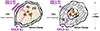 |
Fig. 1. Clump-envelope structure of a molecular cloud in an environment of (a) high metallicity and (b) low metallicity, suggested by Koda et al. (2022) based on previous studies (e.g., Maloney & Black 1988; Wolfire et al. 2010). In the low-metallicity environment (b), CO molecules are selectively photo-dissociated in the envelope (orange) by the external UV radiation field, producing a thick CO-deficient H2 layer (gray), which substantially reduces the CO(2–1) and CO(1–0) emission. The dense star-forming clumps (brown and their immediate surroundings) reside at the hearts of the clouds; the CO molecules are protected there, and the clumps can remain bright in CO(3–2). |
This hypothesis is testable by two means. First, the sizes of the dense clumps would be smaller than the typical size of molecular clouds. For example, the Orion A cloud has a diameter of 20 pc (Nakamura et al. 2019). This size could not be resolved at the 1″ (20 pc) resolution of the previous CO(3–2) observations in the M83 XUV disk (Koda et al. 2022), but it can be resolved at a higher-resolution in CO(3–2) with the new observations presented in this paper.
Second, the dense clumps should emit CO(2–1) as well, but it is expected to be faint. If the gas is thermalized at the high nH2 and Tk required for the substantial CO(3–2) excitation, the CO 3–2/2–1 ratio in surface brightness temperature would be close to one, and the CO 3–2/2–1 intensity ratio would be ICO(3 − 2)/ICO(2 − 1) = 2.25 (see more detailed calculations in Sect. 6). This can be tested with deep CO(2–1) observations in conjunction with the measured CO(3–2) fluxes. Such CO(2–1) observations were approved in ALMA Cy9, but were not executed due largely to the loss of observing times in small array configurations as a result of the cyberattack in 2022–2023. In this work, we reevaluate the significance of the upper limit in CO(2–1) flux from the previous non-detection.
3. Observations and data reduction
We observed a region with an approximate diameter of 30″ with the ALMA 12-m array in CO(3–2) and dust continuum emission (project # 2022.1.00359.S in Cycle 9, hereafter Cy9). It is located at a galactocentric distance of ∼1.24R25 (∼8.0′, ∼10.4 kpc). The observed region is covered with 3 pointings in CO(3–2). Figure 2 shows the region with the sensitivity contours at 70, 50, and 30% of the peak sensitivity at the center, which is (RA, Dec)J2000 = (13 : 37 : 05.18, −29:59:53.6). This region is selected based on previous ALMA observations: starting from the CO(2–1) observations of a 2 × 4 kpc2 region (Bicalho et al. 2019, # 2013.1.00861.S in Cycle 3, Cy3), and the 1 kpc2 subregion studied in CO(3–2) (the gray scale image in Fig. 2; Koda et al. 2022, # 2017.1.00065.S in Cycle 7, Cy7). Within the 1 kpc2 region, a smaller region is selected for this work. This region has bright UV and Hα peaks and multiple molecular clouds (Fig. 2).
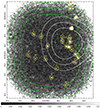 |
Fig. 2. Field of view (FoV) of Cy9 (white contours) with respect to that of Cy7 (green), displayed on the CO(3–2) peak intensity map of the Cy7 data imaged with natural weighting (CY7NA). The FoV center of Cy9 is at (RA, Dec)J2000 = (13:37:05.18, −29:59:53.6). The sensitivity decreases outward from the centers for both FoVs, and the contours show the locations of 70, 50, and 30% of the peak sensitivity for the Cy7 (green) and 9 data (white). The 11 clouds within the 50% white contour are the focus of this paper. The yellow circles have 2″ (44 pc) diameters and mark the locations of the 23 molecular clouds in Koda et al. (2022). The colorbar is in units of Jy/beam. |
We analyzed the Cy3, Cy7, and Cy9 data. The details of the Cy3 and Cy7 observations are in Koda et al. (2022). In the new Cy9 observations, we configured one spectral window for the CO(3–2) line emission with band and channel widths of 937.5 MHz (812.8 km s−1) and 564.5 kHz (0.4894 km s−1). The other three spectral windows were configured to cover different sky frequencies for the continuum emission with a bandwidth of 1.875 GHz with 128 channels per spectral window. The central frequency of the continuum emission in the combination of the Cy7 and Cy9 data is 351.3 GHz (hereafter, 351 GHz continuum emission). The final uv-coverage at the CO(3–2) frequency ranges over angular scales of 0.23–12.2″ (∼5.0–266 pc).
The visibility data are calibrated using the data reduction scripts provided by the ALMA Observatory using the Common Astronomy Software Application (CASA; McMullin et al. 2007; CASA Team 2022). The amplitude and phase of the bandpass and gain calibrators are confirmed to be flat over time and frequency after the calibrations.
For imaging, we used the Multichannel Image Reconstruction, Image Analysis, and Display package (MIRIAD; Sault et al. 1995, 1996). The CO(3–2) data from Cy7 and Cy9 were imaged separately and together. We used the natural (NA) and uniform (UN) weightings. The parameters for the imaging and final data cubes are listed in Table 1. Depending on the dataset and weighting, we refer to each data cube as CY7NA, CY7+9NA, CY7+9UN, and so on (see Table 1). The RMS noise per channel is calculated using the dirty cubes before deconvolution in the areas where the primary beam attenuation is practically negligible (PB > 0.95). Since the sensitivity and beam shape vary in an asymmetric way across the field of the Cy7 and Cy9 combined data, CY7+9NA and CY7+9UN, they are used only for reference, but not for measurements.
Parameters of the reduced data cubes.
Table 1 includes the coefficient to convert intensity/flux units from Jy/beam to K. In this paper we mainly use Jy/beam since the sources are not resolved (only marginally resolved at best; see Sect. 5).
4. Cloud and clump identifications and parameters
We identified clouds and clumps hierarchically, first finding objects in the CY7NA cube and then searching for their substructures in the CY9NA cube by limiting the search within the volumes of the CY7NA objects, doing the same with the CY9UN cube within the volumes of the CY9NA objects. We adopted this approach because the CY7NA data have the highest sensitivity, albeit the lowest spatial resolution (see Table 1). Once the volumes of the objects were restricted by the CY7NA analysis, we relaxed search thresholds in the CY9NA and CY9UN data that have higher resolutions but lower sensitivities (see the details below). To remove the effects of sensitivity variations across the observed fields, we generated and used signal-to-noise ratio (S/N) cubes for the identifications. Unless stated otherwise, we adopted the cubes with a 2.54 km s−1 channel width.
We refer to the objects identified in the CY7NA cube as clouds and those in the CY9NA and CY9UN cubes as clumps. These names reflect only the spatial resolutions of the data used for their identifications. The CY7NA cube has a resolution of 0.89″ (19 pc), approximately the diameter of a molecular cloud, and the CY9NA and CY9UN cubes have 0.40″ (8.6 pc) and 0.28″ (6.1 pc), respectively, tracing sub-cloud scales.
4.1. Clouds
Twenty-three molecular clouds were previously identified by Koda et al. (2022) in the same Cy7 data with an earlier data reduction. For the sake of consistency, we repeated the same identification procedure on the new CY7NA data (2.54 km s−1 channel width). In the S/N cube, we first find pixels with > 5σ significance and extend their volumes down to pixels with 3σ per channel. In some cases, the envelopes of two clouds overlap, which are split with the watershed algorithm (CLUMPFIND; Williams et al. 1994). We find the same set of 23 molecular clouds as in Koda et al. (2022).
This cloud identification defines a volume of each cloud in the three-dimensional data cubes, which is used as a mask for the clump identification in the next subsection.
Hereafter, we discuss only the clouds within the Cy9 field of view (to the 50% level of the primary beam), which includes eleven clouds (Clouds 4, 7, 8, 9, 10, 11, 12, 13, 14, 15, and 17; see Fig. 2). Figures A.1 and A.2 show their cutout images in integrated intensity and peak intensity, respectively. The clouds are arranged from left to right, with their ID#s in the top-left corners. They are also shown from several different imaging runs in CY7NA, CY7+9NA, CY7+9UN, CY9NA, and CY9UN. These 11 clouds are listed in Table A.1 (the full list of the 23 clouds is in Table A.2). Cloud ID is labeled in the format “XX”.
None of the eleven clouds is above the 3σ detection limit in the CO(2–1) line and 351 GHz continuum emission. Figure 3 shows the S/N images calculated from the peak intensity maps: (a)(b) CO(3–2), (c) CO(2–1), and (d) 351 GHz continuum. The CO(2–1) emission is not convincingly detected even in a stack analysis of the 11 cutout images (see Appendix B).
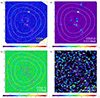 |
Fig. 3. S/N images in peak intensity: (a) CY9NA – CO(3–2), (b) CY7+9NA – CO(3–2), (c) CY3NA – CO(2–1), and (d) CY7+9CONT – 351 GHz continuum. The white contours show the locations of 70, 50, and 30% the peak sensitivity for the Cy9 data. The magenta circles have diameters of 2″ (44 pc) and mark the locations of the clouds; the cloud IDs are given above each circle. |
4.2. Clumps (Level A and B)
We first searched the CY9NA cube, finding clumps within the cloud volumes identified in CY7NA (in the CY7NA mask), and then searched the CY9UN cube to find clumps within the volumes of the CY9NA clumps. To differentiate them, the first group of CY9NA clumps is called “Level A clumps”, and the second group, from CY9UN, is “Level B clumps”. Level B clumps reside within the volumes of Level A clumps and are their substructures. We adopted the same identification procedure as for the clouds (Sect. 4.1) but limited the search volumes.
For Level A clumps, we started from the CY9NA cube and applied the CY7NA mask to limit the search range within the volume of the CY7NA clouds. Since this is the volume where a cloud exists at a higher significance, it is less likely to pick up noise even with a lenient detection threshold. Hence, we started from > 4σ peaks and extended them to the 3σ envelopes. In the CY9NA cube, we detect one or two clumps within all the clouds except Clouds 11 and 17. These two clouds are near the edge of the Cy9 field of view (Fig. 2), where the sensitivities are compromised due to the primary beam attenuation. In Table A.1, the eleven CY9NA clumps are labeled in the format “XX − YY” with “XX” as the parental cloud ID and “YY” as the clump ID within the cloud.
For Level B clumps, we did the same as for the CY9UN cube, using the same detection thresholds, but within the volumes of the CY9NA clumps as masks. The CY9UN cube has the lowest sensitivity among the CO(3–2) data cubes (Table 1) and can identify only the brightest clumps, and yet at the highest spatial resolution. We find nine CY9UN clumps. They are listed in Table A.1 with the IDs labeled in the format “XX − YY − ZZ”.
Clouds 4 and 10 are resolved to two clumps 4-1 and 4-2, and 10-1 and 10-2, respectively. Clump 4-2 is resolved further into three clumps, 4-2-1, 4-2-2, and 4-2-3.
4.3. Parameters
Tables A.1 and A.2 lists the measured parameters of the clouds and clumps, including their ID; positions in RA, Dec, and velocity; full width half maximum (FWHM) sizes in RA (=x), Dec (=y), and recession velocity (=v) directions; peak brightness temperature Tp, peak intensity Ip and its uncertainty ΔIp; the integrated flux F and its uncertainty ΔF; the velocity dispersion σv and its uncertainty Δσv; and the primary beam attenuation (the fraction with respect to the peak sensitivity). We used the CY7NA, CY9NA, and CY9UN cubes and masks for the measurements of the CY7NA clouds and the CY9NA and CY9UN clumps, respectively. We adopted the cubes of the 2.54 km s−1 channel width for these measurements except for FWHMv (and σv), for which we used 0.85 km s−1 cubes.
As explained, cloud and clump ID are labeled in a hierarchical manner. The substructures inherit the labels of their parental structures: “XX” for the CY7NA clouds, “XX − YY” for the CY9NA (Level A) clumps, and “XX − YY − ZZ” for the CY9UN (Level B) clumps.
The coordinates are the intensity-weighted centroid positions.
The Npix is the number of the pixels identified in a cloud or clump in the RA-Dec-Vel volume (i.e., x − y − v volume). Nxy is the number of the pixels in the RA-Dec projection (x − y plane). Some clumps show Npix = Nxy, meaning that they are detected in one velocity channel. For reference, the areas of the beams (Table 1) correspond to Nxy = 356.8 (CY7NA), 70.6 (CY9NA), and 35.4 (CY9UN), respectively.
The FWHMs are calculated from the dispersions  (where i = x, y, v) within the cloud volume in the cube, assuming Gaussian profiles in space and velocity, as
 (1)
(1)
Table A.1 lists FWHMis instead of  , because they are directly comparable to the beam sizes. We used the 0.85 km s−1 cubes for FWHMv; we re-gridded the masks from the 2.54 km s−1 cubes and applied them to the 0.85 km s−1 cubes before taking the measurements.
We note that the beam sizes are different for the CY7NA clouds, CY9NA clumps, and CY9UN clumps (Table 1). FWHMs in Tables A.1 and A.2 are the measured values before dilution corrections for the beam size and velocity resolution.
The Ip and F are the values corrected for primary beam attenuation. Ip is also written in the form of the brightness temperature, Tp, in kelvins, converted with the Rayleigh-Jeans equation. ΔIp is from the RMS noise in Table 1. ΔF was calculated with the standard noise propagation starting from ΔIp by taking into account the number of beams in the volume of objects.
The S/N (Ip/ΔIp) can be calculated from Table A.1. Level A (CY9NA) clumps are detected at peak S/N ratios of 4–15, mostly at S/N > 5 with the exceptions of Clumps 10-2, 15-1, and 7-1 (S/N = 4–5). Level B (CY9UN) clumps are detected less significantly, mostly in the range S/N = 4–6 except 4-1-1 (S/N = 9.9). Figures A.1 and A.2 show their integrated intensity and peak intensity maps.
From these measured parameters, we calculated the radius, R, and velocity dispersion, σv, of the clouds and clumps. The observed  and FWHMi contain the beam size or velocity channel width. To remove their effects, we calculated the second moments in radius and velocity as
 (2)
(2)
 (3)
(3)
and
 (4)
(4)
The σch2 is the second moment of the channel window function (channel shape), and  for a top-hat function with a full width of w. We measured the σv and FWHMv with the cubes of w = 0.85 km s−1. For R, we used Eq. (4), the definition by Solomon et al. (1987), which is supposed to represent the whole radial extent of the object.
Equation (2) requires the measured FWHMx and FWHMy to be greater than bmaj and bmin (beam size) and the σr and R to be positive. This condition is met only for Cloud 4 and Clump 13-1, and even their R ( = 0.35″ and 0.20″ respectively) are less than half the beam sizes. Therefore, we consider that none of the clouds nor the clumps are spatially resolved in any of the measurements. We followed Koda et al. (2022) to set the upper limit of their size and considered R to be measurable only when the measured size is at least 20% larger than the beam size. The minimum measurable radius is then  . This is 0.50″ (10.9 pc), 0.22″ (4.8 pc), and 0.16″ (3.5 pc) for the clouds (CY7NA), Level A clumps (CY9NA), and Level B clumps (CY9UN), respectively. Obviously, these minimum radii correspond to the diameters of 1.00″ (21.8 pc), 0.44″ (9.6 pc), and 0.32″ (7.0 pc), respectively.
The R (upper limit) and σv are listed in Table A.1.
5. Small sizes of CO(3–2) clumps
Our hypothesis is that the CO(3–2) emitting regions are dense clumps embedded in the CO-deficient cloud envelopes (Fig. 1 and Sect. 2). If this is correct, the CO(3–2) emitting regions should be compact compared to typical cloud sizes. In what follows, we show that the CO(3–2) emitting regions are indeed compact and are not spatially resolved (or at most, are only marginally resolved) in the new data, based on a consideration of the measured sizes, peak intensities, and total fluxes of the clouds and clumps.
5.1. Size measurements
Figures A.1 and A.2 show the clouds and clumps, from the top to bottom panels, at the lowest (0.89″, 19 pc for CY7NA) to highest resolutions (0.40″, 8.7 pc for CY9NA and 0.28″, 6.1 pc for CY9UN). The yellow circles have a diameter of 2″ (44 pc), which is close to a typical diameter of giant molecular clouds, 40 pc, in the Milky Way (Scoville & Sanders 1987). We recall that the clouds are identified in the CY7NA data, and Level A and B clumps are in the CY9NA and CY9UN data, respectively.
Clouds 4 and 10 are formally resolved into smaller clumps by the identification criteria in Sect. 4.2. None of these clumps are resolved at the higher resolutions (Table A.1). By eye, clouds 13 and 17 could also be split into smaller clumps, but are not formally resolved with the identification criteria. Their apparent clumps appear to be as small as those in cloud 4 (Figs. A.1 and A.2). The other clouds have only a single, unresolved clump (Table A.1).
Quantitatively, in Table A.1, the FWHMx and FWHMy of the clouds are similar to the beam size of the CY7NA data (0.89″, 19 pc). This linear spatial scale is close to the sizes of small molecular clouds in the Milky Way disk. FWHMx and FWHMy of Level A and B clumps are also similar to the beam sizes of CY9NA and CY9UN (0.40″, 9 pc and 0.28″, 6 pc, respectively). Hence, they are not spatially resolved even at the higher resolutions.
From this, we conclude that the CO(3–2) emitting clumps in each cloud are not spatially resolved at the beam sizes of CY9NA and CY9UN. We note that our size measurements are not very accurate because our clump detection thresholds are not high: S/N > 4 and > 3 at the peak and envelope. Within the uncertainties, the CO(3–2) sources appear to be as compact as the beam sizes of ∼6–9 pc or possibly smaller.
5.2. Implications of the peak intensities and fluxes
Table 2 compares the peak intensities (top part) and total fluxes (bottom) between the parental clouds and their clumps (both Level A and B clumps). Each row gives measurements within each cloud. The peak intensity of the clumps, max(Ip), is that of the brightest clump within the cloud. The total flux of the clumps, ∑F, is the sum of the fluxes of all the identified clumps in the cloud. Table 2 also lists their ratios (i.e., the fractions of emission in the clumps over that in the cloud).
Comparison of clouds and Level A and B clumps in terms of peak intensity and total flux.
Figure 4a shows the peak intensity ratio between the brightest clump in a cloud and the parental cloud (columns 4 and 6 in the top part of Table 2). The red squares are for Level A clumps, and the blue circles are for Level B clumps. In all cases, this ratio is as high as ∼50–100% with the averages of 77% for Level A and 68% for Level B. The peak intensity Ip represents a flux within a beam area at the peak position within an object; and the beam sizes are different between the cloud (0.89″) and clump measurements (0.40″ or 0.28″). The high ratios indicate that approximately the same amount of flux is enclosed within the large and small beams, and hence, the CO(3–2) sources are not much spatially resolved even with the small beams. This supports the hypothesis that the CO(3–2) emission comes from a small region within a cloud. The resolved clouds (especially # 10 and 13) have relatively low fractions because the cloud flux is split into the fluxes of the multiple unresolved clumps, and this measurements take only one of them (the brightest) into account.
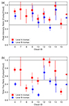 |
Fig. 4. Clumps over cloud ratios for Level A (red square) and B clumps (blue circle) measured in CO(3–2). (a) Peak intensity ratio. The peak intensity of the brightest clump, max(ℐp) in mJy/beam(1), is compared with the peak intensity of its parental cloud, Ip, in mJy/beam(2). Note that the two beams (1 and 2) have different sizes. (b) Total flux ratio. On the right edge of each panel, the triangles pointing left show the averages of the Level A (red) and B (blue) clumps. |
Figure 4b shows the fraction of the total flux of all clumps over that in their parental cloud (columns 4 and 6 in the bottom part of Table 2). An overall trend of this fraction appears different between Level A and B clumps. For Level A (red squares), the fraction is high and is mostly ∼50–100%, with exceptions of clouds 8 and 15 where it is 30 and 21%, respectively. The areal ratio of the CY7NA and CY9NA beams is (0.40″/0.89″)2 ∼ 0.2, and hence, the fraction would be 20% if the emission is uniformly distributed within the CY7NA’s 0.89″ beam. The measured fractions of ≫20% suggest that the CO(3–2)-emitting regions are concentrated mostly in the CY9NA’s 0.40″ beam. For Level B (blue circles), the fraction decreases to ∼10–50% except for cloud 12. The decreasing trend from the low to high resolutions may indicate that the clumps are starting to be resolved between the resolutions of CY9NA (0.40″, 8.7 pc) and CY9UN (0.28″, 6.1 pc). In fact, the fraction of Level B over Level A in total flux is ∼30–70% (column 7 in Table 2 bottom). This is similar to the areal ratio of the CY9NA and CY9UN beams, (0.28″/0.40″)2 ∼ 0.5. Therefore, the CO(3–2)-emitting clumps may be being resolved at the resolutions of ∼0.28–0.40″ (6–9 pc).
We should note a couple of caveats. The above discussion is to capture the average characteristics of the observed clouds and clumps, and there are clearly some variations among them. For example, the small total flux fractions of Level A clumps over clouds 8 and 15 may indicate that there are some CO(3–2) emission outside the unresolved clumps. We also caution that interferometer imaging without short spacing data (or with the uniform weighting) often reduces the apparent flux. This is because the emission contained in those data is missed, and also because they carry the flux information and their weight reduction causes systematic uncertainties in the imaging process. However, the overall trends discussed above suggest that, on average, the CO(3–2)-emitting objects are smaller than the typical sizes of Galactic molecular clouds.
We draw the same conclusion from the peak surface brightness temperature Tp. Table A.1 shows that Tp generally increases from the low-resolution (CY7NA) to high-resolution data (CY9UN), indicating that the objects are unresolved, but are approaching to be resolved. The CO emission easily becomes optically thick on theoretical and empirical bases (Goldreich & Kwan 1974; Solomon et al. 1979), and thus, we assumed that it is optically thick. Using the beam filling factor f (i.e., the areal fraction of an object over beam), Tp is related to the excitation temperature T32 as Tp = [fΓ(ν32, T32)]T32 (see Eq. (6) for Γ). Γ is an increasing function of T32 and can be evaluated numerically. This gives Tp = (3.9f − 22.5f) K for T32 = 10–30 K with f as an unknown factor. Compared to Tp in Table A.1 (the brightest is Clump 4-1-1 with Tp = 2.49 K), the filling factor is f = 0.64 or smaller, again indicating unresolved or marginally resolved objects. The CO emission rarely becomes optically thin, except under some very special conditions (e.g., line wings and extremely low metallicity); thus, we did not consider it further but briefly note that an optically thin case would reduce the apparent Tp and, hence, make the above f a lower limit.
6. Non-detection in CO(2–1)
The combination of the detection in CO(3–2) and non-detection in CO(2–1) also constrains the cloud structure and physical condition. The new data reduction of the CO(2–1) also supports this.
Koda et al. (2022) assumed, as in Fig. 1b, that [1] the cloud envelope is CO-deficient due to the low metallicity and does not emit much CO emission, while the dense clump(s) in the cloud is still CO-rich and emit CO(3–2) as well as CO(1–0) and CO(2–1), and [2] the CO-rich part of the cloud (i.e., the dense clumps) is close to being thermalized, and hence, the CO 3–2/2–1 ratio in surface brightness temperature is relatively high and is approximately unity. Under these assumptions, the CO(2–1) flux can be predicted from the observed CO(3–2) flux. Koda et al. (2022) concluded that the predicted CO(2–1) flux of the brightest cloud is just below the detection limit of the previous CO(2–1) observations (Bicalho et al. 2019). We note that in this section, we discuss “flux” instead of “surface brightness temperature” because the emission sources are not resolved.
The assumptions that Koda et al. (2022) adopted predict the minimum of the CO(2–1) flux. In other words, if any of the assumptions deviate significantly from the reality, the predicted CO(2–1) flux would be higher and should have been detected in the previous CO(2–1) study.
The CO(2–1) flux of a CO(3–2)-emitting dense clump, without the cloud envelope, can be estimated from its CO(3–2) flux. We assumed that the beam filling factors of the two transitions are equal. Using the flux Fi, excitation temperature Ti, and frequency νi of the CO(2–1) and CO(3–2) emission (i = 21 or 32, respectively), the CO 3–2/2–1 flux ratio is
 (5)
(5)
where
 (6)
(6)
and we defined
 (7)
(7)
The “T21/T32” term in Eq. (5) takes the minimum under the thermalized condition (T21 = T32) with respect to non-thermalized conditions (T21 > T32). The “α” term can be evaluated numerically and is always α(T21 > T32) > α(T21 = T32), taking the minimum in the thermalized condition. Therefore, using αth(T)≡α(T ≡ T21 = T32), the thermalized condition always predicts the minimum CO(2–1) flux of F21 = (4/9αth(T))F32, where αth≈1.10, 1.16, and 1.40 for T = 30, 20, and 10 K, respectively. Here, we neglected the contribution of the cosmic microwave background radiation since its temperature is low for the CO(3–2)-emitting gas.
The brightest cloud (Cloud 4 in Table A.1) has the CO(3–2) flux of  . In the thermalized condition, this translates to the minimum expected CO(2–1) flux of F21 = 126.2, 133.1, and 160.7 mJy km s−1 at 30, 20, and 10 K (Eq. (5)). This cloud has FWHMv = 6.21 km s−1 in CO(3–2), and if this is also the width in CO(2–1), the minimum predicted CO(2–1) intensity is I21 = 20.3, 21.4, and 25.9 mJy. These are at 1.9, 2.0, and 2.4σ significance, respectively. Thus, it is slightly below the detection limit of the existing CY3NA data.
If the clump is not thermalized, the predicted CO(2–1) flux becomes higher and should have been detected. For example, if the CO(3–2)-emitting region has T32/T21 ∼ 0.5 (i.e., the average in the main disks of nearby galaxies; Leroy et al. 2022), α(T21, T32) = α(T, T/2) = 1.51, 1.92, and 4.39 at T = 30, 20, and 10 K. Cloud 4 would have F21 = 346.6, 440.7, and 1007.6 mJy km s−1 and I21 = 55.8, 71.0, and 162.2 mJy. It should have been detected in CO(2–1) at 5.2, 6.6, and 15.2σ in the CY3NA data. Therefore, the excitation condition of the clump cannot deviate significantly from the thermalized condition, given the non-detection in CO(2–1).
In addition, if the envelope of the cloud is filled with CO, the CO(2–1) flux would be higher since the CO(2–1) emission is easily excited in the average density and temperature of typical cloud envelopes. This should also have made the clump detectable in the previous study.
In summary, the non-detection in CO(2–1) supports the cloud structure presented in Fig. 1b. This is obviously a simplistic picture, and the details will need some modification in the future. However, as a first order approximation, Fig. 1b likely represents the cloud structure in the XUV disk.
7. The size–velocity dispersion relation
Figure 5 plots σv against the upper limits of R for the clouds (arrows at log R = 1.03), Level A (0.68) and B clumps (0.54). For reference, it also shows clouds in the Milky Way, Large and Small Magellanic Clouds (LMC and SMC), and the dwarf galaxy WLM (Solomon et al. 1987; Bolatto et al. 2008; Wong et al. 2011; Rubio et al. 2015). The clouds in the XUV disk of M83 appear consistent with those in the dwarfs, while their radii are only upper limits.
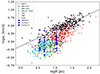 |
Fig. 5. σv − R plot. M83 XUV disk clouds and clumps are in blue (and the blue arrows are the upper limits in radius). The clouds have the largest radii, followed by the Level A and then the Level B clumps. The reference points in the background are for the Milky Way’s inner disk (Solomon et al. 1987), outer disk (rgal∼12–14 kpc; Sun et al. 2017), and far outer disk (∼14–22 kpc; Sun et al. 2015), the LMC and SMC (Wong et al. 2011; Bolatto et al. 2008), and WLM (Rubio et al. 2015). The solid line is a fit to the inner disk clouds (Solomon et al. 1987). |
There is also a caveat in this comparison, since these reference clouds are observed in the lower-excitation transitions, CO(1–0) or CO(2–1). However, we note that the three CO transitions (J = 1–0, 2–1, and 3–2) should be emitted from a similar central region (Fig. 1b) if the clouds and clumps share a similar physical and chemical structure in the low-metallicity environments (i.e., the Milky Way outskirts, LMC, SMC, and other dwarfs, as well as the XUV disk). In fact, molecular clouds in LMC and SMC appear compact in recent CO(1–0) and CO(2–1) measurements (Harada et al. 2019; Tokuda et al. 2021; Ohno et al. 2023). Therefore, the consistency in Fig. 5 supports our hypothesis (Fig. 1), of course, within the limitation that we have only the upper limits of R.
8. Further discussion
Koda et al. (2022) presented a hypothesis on the mass structure and CO chemistry in molecular clouds in the XUV disk (Fig. 1). The Orion A cloud (i.e., a nearby Galactic molecular cloud) exhibits SF activity similar to those around the XUV disk clouds, and it consists of a relatively low-density envelope of ∼20–30 pc with a dense CO(3–2)-bright region of ∼10 pc in size (Ikeda et al. 1999); Nakamura:2019wt. The hypothesis suggests that the XUV clouds also have a similar mass structure, but in their envelopes, CO molecules are photo-dissociated and deficient due to the low metallicity condition. The dissociating UV radiation is in the XUV disk (see Koda et al. 2022; there are multiple Orion-like sites of massive SF – traced by UV and Hα sources – in the 1 kpc2 region, i.e., the Cy7 field of view). This study confirms the compactness of the CO(3–2)-emitting regions (≲6–9 pc in diameter) in the XUV disk clouds. In the Orion A cloud, the dense CO(3–2)-bright region consists of multiple smaller clumps (see Ikeda et al. 1999), while our resolution is not high enough to resolve such substructures. This study also shows that the CO(3–2)-emitting regions in the XUV disk clouds must be close to the thermalized condition, since otherwise the expected CO(2–1) flux would be brighter and should have been detected in the past ALMA observations.
8.1. Mass and radius of the CO(3–2)-emitting regions
The masses of the clumps (i.e., CO(3–2)-emitting regions) can be crudely estimated (Koda et al. 2022), assuming that (1) the clumps have CO molecules (as in Fig. 1b), (2) the Galactic CO-to-H2 conversion factor XCO(1 − 0) = 3 × 1020 cm−2 [K km s−1]−1 can be applied to the clumps (i.e., parts of the clouds)1, and (3) the gas is thermalized and hence the CO 3–2/1–0 brightness temperature ratio is unity (R3 − 2/1 − 0 = 1). With these assumptions, the clump mass, including helium and other heavier elements (i.e., multiplying the total hydrogen mass by 1.37), is
 (8)
(8)
The measured CO(3–2) fluxes (Table A.1) give Mclump = 2.1 × 10² − 9.3 × 10³ M⊙.
These Mclump can be translated, also crudely, to the radius of clumps (or clump concentrations). The CO(3–2) excitation requires a density of  , to within an order of magnitude. By assuming this density as an average density in a spherical CO(3–2)-emitting region, the clump mass within its radius, including helium and other heavier elements, is
 (9)
(9)
The range of the clump masses estimated above then corresponds to R = 1–4 pc. This is consistent with the new measurements in this study. The clumps (or their concentrations) are compact and not spatially resolved at the 6–9 pc resolutions, while there is an indication that they may be starting to be resolved at the 6 pc resolution.
These mass estimations easily have a factor of 2-3 uncertainty. It is also worth noting that, within such uncertainties, they are roughly consistent with the virial mass Mvir ( = 9/2(Rσv2/G) for a radial density profile of ∝1/r; see Lee et al. (2024), which is
 (10)
(10)
using rounded values of R = 3 pc and  (see Table A.1).
8.2. Cloud evolution and distribution
The cloud structure in Fig. 1 does not take into account the evolution of molecular clouds. It is possible that the clouds evolve and develop dense clumps only at a later stage of their lifetime. In this case, the CO(3–2) observations would selectively trace the clouds at the evolved stage when they are ready for SF. In fact, in the inner disk of M83, the populations of star-forming molecular clouds are mostly localized around the galactic center, bar, and spiral arms. Molecular gas and clouds are abundant even in the interarm regions, but appear to be dormant in SF (Koda et al. 2023). If this is also the case in XUV disks, there could also be (undetected) clouds at an earlier stage of their evolution before the dense clumps develop in their hearts. In order to understand the SF in XUV disks and in general, it is important to confirm the presence or absence of such dormant cloud populations and to characterize their structures and distribution as a function of their environments (e.g., the amount of the surrounding HI gas, spiral arms, UV radiation field, stellar feedback, etc.).
The large-scale distribution of the clouds may also provide a clue on their formation and evolution (e.g., Dobbs & Baba 2014). Two additional clouds emerge at the highest sensitivity part of the CY7+9NA data (see Fig. 3b), while we focused on the clouds and clumps discovered in the CY7NA data. One is detected at 6.3σ between Clouds 9 and 12 at a peak position of (RA, Dec) = (13:37:05.29, −29:59:54.1), and the other is at 5.3σ between Clouds 7 and 8 at (13:37:05.18, −29:59:50.7). The CY7+9NA data, however, have a nonuniform, asymmetric sensitivity distribution (Fig. 2), and thus, we did not include them in the sample for our analysis. Nevertheless, they exemplify the fact that more CO(3–2) sources could emerge with longer integration. Koda et al. (2022) noted that the CO(3–2) sources are distributed along filamentary structures as chains (like seeds in edamame green soybeans). The two CY7+9NA clouds appear to support this view. The distribution may indicate that their formation requires compression due to large-scale gas flows.
9. Summary
Massive SF sites have been detected in XUV disks, but their parental gas clouds remained mostly undetected despite searches in CO(1–0) and CO(2–1). Therefore, the recent discovery of 23 molecular clouds in CO(3–2) in the XUV disk of M83 is startling. To explain the previous non-detections and the new detections, Koda et al. (2022) introduced the hypothesis that clouds in XUV disks, like Galactic star-forming clouds, have dense star-forming clumps embedded in a large envelope of bulk molecular gas, where CO molecules are photo-dissociated due to the lack of CO self-shielding and dust extinction in the low-metallicity environment of XUV disks (Figs. 1a,b). CO(3–2) can be excited preferentially in the dense clumps but not as much in the less dense envelopes. This can explain why CO(3–2) is detected when CO(1–0) and CO(2–1) levels are significantly reduced.
This paper confirms the compactness of the dense, CO(3–2)-emitting clumps in the clouds as predicted by this hypothesis. In the new ALMA data, they are not resolved at a 0.40″ (9 pc) resolution (natural weighting), nor at a 0.28″ (6 pc) resolution (uniform weighting), but there is some indication that they may be starting to be resolved at the 6 pc resolution. These are similar to the sizes of the dense central clumps (or their concentration) in the Orion A molecular cloud in the solar neighborhood, where a similar amount of massive SF is ongoing.
The CO(3–2) to CO(2–1) and CO(3–2) to CO(1–0) line ratios in the dense clumps must be higher than the average ratio observed in normal galactic disks (e.g., T32/T10 ∼ 1/3 and T32/T21 ∼ 1/2; Wilson et al. 2009; Vlahakis et al. 2013; Leroy et al. 2022). Otherwise, the previous study (Bicalho et al. 2019) would have detected the CO(2–1) emission. Likewise, the molecular envelopes around the dense clumps within the clouds cannot have much CO, as the CO(1–0) and CO(2–1) emission should be excited easily in the envelopes and, thus, would have been detected. The CO(3–2)-emitting regions in the XUV clouds must be close to thermalized since, otherwise, the CO(2–1) flux would be brighter and thus would have been detected in past observations.
The cloud structure hypothesized here is, of course, simplistic and will need some adjustments in the future. For example, it does not include the possible evolution of clouds from a non-star-forming phase to a star-forming phase. The clouds detected in CO(3–2) may trace only the clouds in the star-forming phase. For the clouds in the XUV disk discussed in this paper, this model appears to capture the reality within the limitation of the current observations.
We assumed this XCO(1 − 0) for clumps. If their parental clouds have the structure in Fig. 1b, their envelopes should have a fair amount of mass while no/little CO emission. Thus, XCO(1 − 0) for clouds should be larger than the assumed, which is the often-discussed metallicity dependence of XCO(1 − 0). Recently, Lee et al. (2024) also pointed out a possible dependence of XCO(1 − 0) on cloud population.
Acknowledgments
JK thanks his colleagues at Paris Observatory for their hospitality, both professionally and personally, during his stay on sabbatical, and colleagues at the Institut d’Astrophysique de Paris for stimulating discussions. We also thank the anonymous referee. This paper makes use of the following ALMA data: ADS/JAO.ALMA#2013.1.00861.S, 2017.1.00065.S, and 2022.1.00359.S. ALMA is a partnership of ESO (representing its member states), NSF (USA) and NINS (Japan), together with NRC (Canada), MOST and ASIAA (Taiwan), and KASI (Republic of Korea), in cooperation with the Republic of Chile. The Joint ALMA Observatory is operated by ESO, AUI/NRAO and NAOJ. Data analysis is in part carried out on the Multi-wavelength Data Analysis System operated by the Astronomy Data Center (ADC) in NAOJ. J.K. acknowledges support from NSF through grants AST-1812847 and AST-2006600. M.R. wishes to acknowledge support from ANID(CHILE) through FONDE-CYT grant No1190684.
References
- Bergin, E. A., & Tafalla, M. 2007, ARA&A, 45, 339 [Google Scholar]
- Bicalho, I. C., Combes, F., Rubio, M., Verdugo, C., & Salome, P. 2019, A&A, 623, A66 [NASA ADS] [CrossRef] [EDP Sciences] [Google Scholar]
- Bigiel, F., Leroy, A., Seibert, M., et al. 2010, ApJ, 720, L31 [NASA ADS] [CrossRef] [Google Scholar]
- Bolatto, A. D., Leroy, A. K., Rosolowsky, E., Walter, F., & Blitz, L. 2008, ApJ, 686, 948 [NASA ADS] [CrossRef] [Google Scholar]
- Braine, J., & Herpin, F. 2004, Nature, 432, 369 [NASA ADS] [CrossRef] [Google Scholar]
- Braine, J., Ferguson, A. M. N., Bertoldi, F., & Wilson, C. D. 2007, ApJ, 669, L73 [NASA ADS] [CrossRef] [Google Scholar]
- Braine, J., Gratier, P., Kramer, C., et al. 2010, A&A, 518, L69 [NASA ADS] [CrossRef] [EDP Sciences] [Google Scholar]
- Braine, J., Gratier, P., Contreras, Y., Schuster, K. F., & Brouillet, N. 2012, A&A, 548, A52 [NASA ADS] [CrossRef] [EDP Sciences] [Google Scholar]
- Bresolin, F., Ryan-Weber, E., Kennicutt, R. C., & Goddard, Q. 2009, ApJ, 695, 580 [Google Scholar]
- CASA Team (Bean, B., et al.) 2022, PASP, 134, 114501 [NASA ADS] [CrossRef] [Google Scholar]
- Dessauges-Zavadsky, M., Verdugo, C., Combes, F., & Pfenniger, D. 2014, A&A, 566, A147 [NASA ADS] [CrossRef] [EDP Sciences] [Google Scholar]
- Dobbs, C., & Baba, J. 2014, PASA, 31, e035 [NASA ADS] [CrossRef] [Google Scholar]
- Eibensteiner, C., Bigiel, F., Leroy, A. K., et al. 2023, A&A, 675, A37 [NASA ADS] [CrossRef] [EDP Sciences] [Google Scholar]
- Gil de Paz, A., Madore, B. F., Boissier, S., et al. 2005, ApJ, 627, L29 [Google Scholar]
- Gil de Paz, A., Boissier, S., Madore, B. F., et al. 2007, ApJS, 173, 185 [Google Scholar]
- Goldreich, P., & Kwan, J. 1974, ApJ, 189, 441 [CrossRef] [Google Scholar]
- Harada, R., Onishi, T., Tokuda, K., et al. 2019, PASJ, 71, 44 [NASA ADS] [CrossRef] [Google Scholar]
- Ikeda, M., Maezawa, H., Ito, T., et al. 1999, ApJ, 527, L59 [NASA ADS] [CrossRef] [Google Scholar]
- Koda, J., Yagi, M., Boissier, S., et al. 2012, ApJ, 749, 20 [NASA ADS] [CrossRef] [Google Scholar]
- Koda, J., Watson, L., Combes, F., et al. 2022, ApJ, 941, 3 [NASA ADS] [CrossRef] [Google Scholar]
- Koda, J., Hirota, A., Egusa, F., et al. 2023, ApJ, 949, 108 [NASA ADS] [CrossRef] [Google Scholar]
- Lee, A. M., Koda, J., Hirota, A., Egusa, F., & Heyer, M. 2024, ApJ, 968, 97 [NASA ADS] [CrossRef] [Google Scholar]
- Leroy, A. K., Rosolowsky, E., Usero, A., et al. 2022, ApJ, 927, 149 [NASA ADS] [CrossRef] [Google Scholar]
- Maloney, P., & Black, J. H. 1988, ApJ, 325, 389 [NASA ADS] [CrossRef] [Google Scholar]
- McMullin, J. P., Waters, B., Schiebel, D., Young, W., & Golap, K. 2007, ASP Conf. Ser., 376, 127 [Google Scholar]
- Nakamura, F., Ishii, S., Dobashi, K., et al. 2019, PASJ, 71, S3 [NASA ADS] [CrossRef] [Google Scholar]
- Ohno, T., Tokuda, K., Konishi, A., et al. 2023, ApJ, 949, 63 [NASA ADS] [CrossRef] [Google Scholar]
- Rautio, R. P. V., Watkins, A. E., Salo, H., et al. 2024, A&A, 681, A76 [NASA ADS] [CrossRef] [EDP Sciences] [Google Scholar]
- Rubio, M., Elmegreen, B. G., Hunter, D. A., et al. 2015, Nature, 525, 218 [NASA ADS] [CrossRef] [Google Scholar]
- Sault, R. J., Teuben, P. J., & Wright, M. C. H. 1995, ASP Conf. Ser., 77, 433 [NASA ADS] [Google Scholar]
- Sault, R. J., Staveley-Smith, L., & Brouw, W. N. 1996, A&AS, 120, 375 [NASA ADS] [CrossRef] [EDP Sciences] [Google Scholar]
- Scoville, N. Z., & Sanders, D. B. 1987, Astrophys. Space Sci. Lib., 134, 21 [NASA ADS] [CrossRef] [Google Scholar]
- Solomon, P. M., Sanders, D. B., & Scoville, N. Z. 1979, ApJ, 232, L89 [NASA ADS] [CrossRef] [Google Scholar]
- Solomon, P. M., Rivolo, A. R., Barrett, J., & Yahil, A. 1987, ApJ, 319, 730 [Google Scholar]
- Sun, Y., Xu, Y., Yang, J., et al. 2015, ApJ, 798, L27 [Google Scholar]
- Sun, Y., Su, Y., Zhang, S.-B., et al. 2017, ApJS, 230, 17 [NASA ADS] [CrossRef] [Google Scholar]
- Thilker, D. A., Bianchi, L., Boissier, S., et al. 2005, ApJ, 619, L79 [Google Scholar]
- Thilker, D. A., Bianchi, L., Meurer, G., et al. 2007, ApJS, 173, 538 [Google Scholar]
- Thim, F., Tammann, G. A., Saha, A., et al. 2003, ApJ, 590, 256 [NASA ADS] [CrossRef] [Google Scholar]
- Tokuda, K., Kondo, H., Ohno, T., et al. 2021, ApJ, 922, 171 [NASA ADS] [CrossRef] [Google Scholar]
- van Dishoeck, E. F., & Black, J. H. 1988, ApJ, 334, 771 [Google Scholar]
- Vlahakis, C., van der Werf, P., Israel, F. P., & Tilanus, R. P. J. 2013, MNRAS, 433, 1837 [NASA ADS] [CrossRef] [Google Scholar]
- Watson, L. C., & Koda, J. 2017, in Outskirts of Galaxies, eds. J. H. Knapen, J. C. Lee, & A. Gil de Paz, 434, 175 [NASA ADS] [CrossRef] [Google Scholar]
- Williams, J. P., de Geus, E. J., & Blitz, L. 1994, ApJ, 428, 693 [Google Scholar]
- Wilson, C. D., Warren, B. E., Israel, F. P., et al. 2009, ApJ, 693, 1736 [NASA ADS] [CrossRef] [Google Scholar]
- Wolfire, M. G., Hollenbach, D., & McKee, C. F. 2010, ApJ, 716, 1191 [Google Scholar]
- Wong, T., Hughes, A., Ott, J., et al. 2011, ApJS, 197, 16 [NASA ADS] [CrossRef] [Google Scholar]
Appendix A: Parameters and cutout images of clouds and clumps
Table A.1 lists the measured parameters of the clouds and clumps (see Sect. 4.3 for explanations). Figures A.1 and A.2 show their cutout images in integrated intensity and peak intensity, respectively.
Table A.2 is the same as the "Clouds" section of Table A.1, but lists all 23 clouds identified in the CY7NA cube. This table does not include the peak brightness temperature Tp. The Ip and Tp are related as Tp = CKIp (see Table 1 for CK).
Measured parameters of clouds and Level A and B clumps in CO(3–2)
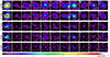 |
Fig. A.1. Cutout images of the clouds and clumps in CO(3–2) integrated intensity. The velocity range of each cloud is integrated. The primary beam correction is applied. From left to right: Different clouds, with their ID# in the top-left corners. From top to bottom: CY7NA, CY7+9NA, CY7+9UN, CY9NA, and CY9UN (see Table 1). The yellow circles have a diameter of 2" (∼44 pc). |
Cloud parameter measurements in CO(3–2) with the CY7NA cube.
Appendix B: The stacked cutout images
A stacking analysis does not provide a significant CO(2–1) detection in this case. The clouds have a large range of flux (Table A.1), and only the brightest ones contribute to the stacked flux, while all the cloud images contribute to the stacked noise.
Figure B.1 shows the stacked CO(3–2) and CO(2–1) images, that is, the sum of the integrated intensity cutout images of the 11 clouds (see Figs. 2 and A.1 and Table A.1). The same velocity ranges are integrated for CO(3–2) and CO(2–1). The beam sizes are different between the two panels (Table 1). If we assume that the (stacked) object is not resolved with either beam, the total flux of the object is the values displayed in these images.
Panel (a) shows the peak CO(3–2) flux of  . The noise of this image is 16 mJy km s−1. The corresponding CO(2–1) flux, predicted under the thermalized condition, is
  (αth ≈ 1.1 at T = 30 K; see Sect. 6 and Eq. 5).
Panel (b) shows a tempting emission peak, but there is also a similarly deep negative just north of it. Indeed, the peak flux is  in CO(2–1), which is apparently consistent with the prediction under the thermalized condition. However, the noise in this image is 140 mJy km s−1. Thus, it is only at a 1.9σ significance. The consistency is supportive of the model (Fig. 1) but is not conclusive with this CO(2–1) data.
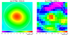 |
Fig. B.1. Stacked (summed) images of the 11 clouds in the Cy9 FoV (see Fig. 2 and Table A.1). (a) CO(3–2) image with CY7NA (with an RMS noise of 16 mJy/beam km s−1). (b) CO(2–1) image with CY3NA (140 mJy/beam km s−1). The white circles have a diameter of 2". Note that the beam sizes are different in the two panels (see Table 1). Assuming that the emission is not resolved, the fluxes in these images indicate the total fluxes of the (stacked) object. |
All Tables
Comparison of clouds and Level A and B clumps in terms of peak intensity and total flux.
All Figures
|
Fig. 1. Clump-envelope structure of a molecular cloud in an environment of (a) high metallicity and (b) low metallicity, suggested by Koda et al. (2022) based on previous studies (e.g., Maloney & Black 1988; Wolfire et al. 2010). In the low-metallicity environment (b), CO molecules are selectively photo-dissociated in the envelope (orange) by the external UV radiation field, producing a thick CO-deficient H2 layer (gray), which substantially reduces the CO(2–1) and CO(1–0) emission. The dense star-forming clumps (brown and their immediate surroundings) reside at the hearts of the clouds; the CO molecules are protected there, and the clumps can remain bright in CO(3–2). |
| In the text | |
|
Fig. 2. Field of view (FoV) of Cy9 (white contours) with respect to that of Cy7 (green), displayed on the CO(3–2) peak intensity map of the Cy7 data imaged with natural weighting (CY7NA). The FoV center of Cy9 is at (RA, Dec)J2000 = (13:37:05.18, −29:59:53.6). The sensitivity decreases outward from the centers for both FoVs, and the contours show the locations of 70, 50, and 30% of the peak sensitivity for the Cy7 (green) and 9 data (white). The 11 clouds within the 50% white contour are the focus of this paper. The yellow circles have 2″ (44 pc) diameters and mark the locations of the 23 molecular clouds in Koda et al. (2022). The colorbar is in units of Jy/beam. |
| In the text | |
|
Fig. 3. S/N images in peak intensity: (a) CY9NA – CO(3–2), (b) CY7+9NA – CO(3–2), (c) CY3NA – CO(2–1), and (d) CY7+9CONT – 351 GHz continuum. The white contours show the locations of 70, 50, and 30% the peak sensitivity for the Cy9 data. The magenta circles have diameters of 2″ (44 pc) and mark the locations of the clouds; the cloud IDs are given above each circle. |
| In the text | |
|
Fig. 4. Clumps over cloud ratios for Level A (red square) and B clumps (blue circle) measured in CO(3–2). (a) Peak intensity ratio. The peak intensity of the brightest clump, max(ℐp) in mJy/beam(1), is compared with the peak intensity of its parental cloud, Ip, in mJy/beam(2). Note that the two beams (1 and 2) have different sizes. (b) Total flux ratio. On the right edge of each panel, the triangles pointing left show the averages of the Level A (red) and B (blue) clumps. |
| In the text | |
|
Fig. 5. σv − R plot. M83 XUV disk clouds and clumps are in blue (and the blue arrows are the upper limits in radius). The clouds have the largest radii, followed by the Level A and then the Level B clumps. The reference points in the background are for the Milky Way’s inner disk (Solomon et al. 1987), outer disk (rgal∼12–14 kpc; Sun et al. 2017), and far outer disk (∼14–22 kpc; Sun et al. 2015), the LMC and SMC (Wong et al. 2011; Bolatto et al. 2008), and WLM (Rubio et al. 2015). The solid line is a fit to the inner disk clouds (Solomon et al. 1987). |
| In the text | |
|
Fig. A.1. Cutout images of the clouds and clumps in CO(3–2) integrated intensity. The velocity range of each cloud is integrated. The primary beam correction is applied. From left to right: Different clouds, with their ID# in the top-left corners. From top to bottom: CY7NA, CY7+9NA, CY7+9UN, CY9NA, and CY9UN (see Table 1). The yellow circles have a diameter of 2" (∼44 pc). |
| In the text | |
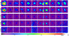 |
Fig. A.2. Same as Fig. A.1, but in peak intensity. |
| In the text | |
|
Fig. B.1. Stacked (summed) images of the 11 clouds in the Cy9 FoV (see Fig. 2 and Table A.1). (a) CO(3–2) image with CY7NA (with an RMS noise of 16 mJy/beam km s−1). (b) CO(2–1) image with CY3NA (140 mJy/beam km s−1). The white circles have a diameter of 2". Note that the beam sizes are different in the two panels (see Table 1). Assuming that the emission is not resolved, the fluxes in these images indicate the total fluxes of the (stacked) object. |
| In the text | |
Current usage metrics show cumulative count of Article Views (full-text article views including HTML views, PDF and ePub downloads, according to the available data) and Abstracts Views on Vision4Press platform.
Data correspond to usage on the plateform after 2015. The current usage metrics is available 48-96 hours after online publication and is updated daily on week days.
Initial download of the metrics may take a while.