| Issue |
A&A
Volume 691, November 2024
|
|
|---|---|---|
| Article Number | A23 | |
| Number of page(s) | 16 | |
| Section | Extragalactic astronomy | |
| DOI | https://doi.org/10.1051/0004-6361/202450892 | |
| Published online | 29 October 2024 | |
Magnetic fields in the outskirts of PSZ2 G096.88+24.18 from a depolarization analysis of radio relics
1
Dipartimento di Fisica e Astronomia, Università di Bologna, Via Gobetti 93/2, I-40129 Bologna, Italy
2
INAF – Istituto di Radioastronomia di Bologna, Via Gobetti 101, I-40129 Bologna, Italy
3
Hamburger Sternwarte, University of Hamburg, Gojenbergsweg 112, 21029 Hamburg, Germany
4
Leiden Observatory, Leiden University, PO Box 9513 NL-2300 RA Leiden, The Netherlands
⋆ Corresponding author; This email address is being protected from spambots. You need JavaScript enabled to view it.
Received:
28
May
2024
Accepted:
13
August
2024
Abstract
Context. Radio relics are diffuse, non-thermal radio sources present in a number of merging galaxy clusters. They are characterized by elongated arc-like shapes and highly polarized emission (up to ∼60%) at gigahertz frequencies, and are expected to trace shock waves in the cluster outskirts induced by galaxy cluster mergers. Their polarized emission can be used to study the magnetic field properties of the host cluster.
Aims. In this paper, we investigate the polarization properties of the double radio relics in PSZ2 G096.88+24.18 using the rotation measure (RM) synthesis, and try to constrain the characteristics of the magnetic field that reproduce the observed depolarization as a function of resolution (beam depolarization). Our aim is to understand the nature of the low polarization fraction that characterizes the southern relic with respect to the northern relic.
Methods. We present new 1–2 GHz Karl G. Jansky Very Large Array (VLA) observations in multiple configurations. We derived the RM and polarization of the two relics by applying the RM synthesis technique, and thus solved for bandwidth depolarization in the wide observing bandwidth. To study the effect of beam depolarization, we degraded the image resolution and studied the decreasing trend of polarization fraction with increasing beam size. Finally, we performed 3D magnetic field simulations using multiple models for the magnetic field power spectrum over a wide range of scales, in order to constrain the characteristics of the cluster magnetic field that can reproduce the observed beam depolarization trend.
Results. Using RM synthesis, we obtained a polarization fraction of (18.6 ± 0.3)% for the northern relic and (14.6 ± 0.1)% for the southern one. Having corrected for bandwidth depolarization, and after noticing the absence of relevant complex Faraday spectrum, we inferred that the nature of the depolarization for the southern relic is external, and possibly related to the turbulent gas distribution within the cluster, or to the complex spatial structure of the relic. The best-fit magnetic field power spectrum, which reproduces the observed depolarization trend for the southern relic, was obtained for a turbulent magnetic field model, described by a power spectrum derived from cosmological simulations, and defined within the scales of Λmin = 35 kpc and Λmax = 400 kpc. This yields an average magnetic field of the cluster within 1 Mpc3 volume of ∼2 μG.
Key words: magnetic fields / magnetohydrodynamics (MHD) / polarization / radiation mechanisms: non-thermal / galaxies: clusters: individual: PSZ2 G096.88+24.18
© The Authors 2024
 Open Access article, published by EDP Sciences, under the terms of the Creative Commons Attribution License (https://creativecommons.org/licenses/by/4.0), which permits unrestricted use, distribution, and reproduction in any medium, provided the original work is properly cited.
This article is published in open access under the Subscribe to Open model. This email address is being protected from spambots. You need JavaScript enabled to view it. to support open access publication.
1. Introduction
Mergers of galaxy clusters are among the most energetic events in the Universe, in which a fraction of the kinetic energy is dissipated into the acceleration of charged relativistic particles, within the hot thermal plasma that fills the clusters, the intracluster medium (ICM). Merger shocks are usually launched along the merger axis, with Mach numbers in the range of M ∼ 2–5 (e.g., van Weeren et al. 2010; Akamatsu & Kawahara 2013; Wittor et al. 2017; Botteon et al. 2020). Despite their low M, these shocks seem to be able to (re)accelerate particles that, with the μG magnetic fields that characterize the clusters’ environment (e.g., Vacca et al. 2018), emit synchrotron radiation at radio frequencies. These structures, known as “radio relics”, represent extraordinary examples of the consequences of the propagation of shocks through the cluster after a cluster-cluster merger (for reviews see Feretti et al. 2012; van Weeren et al. 2019).
Radio relics are mostly found in the outskirts of galaxy clusters and are characterized by elongated shapes, with lengths of 0.5–2 Mpc, and strong polarization at gigahertz frequencies (≳20%, e.g., Enßlin et al. 1998; Stuardi et al. 2022). Relics are among the most polarized sources in the extragalactic sky: the polarization fractions can reach ∼60% in some cases. This high degree of polarization is expected in sources that trace edge-on shock waves (Enßlin et al. 1998). These source properties suggest the presence of large-scale magnetic fields that have intensities of 0.1– , tangled on scales ranging from a few kiloparsecs to hundreds (Brüggen 2013).
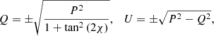
Another way in which the presence of the cluster magnetic field is unveiled is the Faraday rotation effect which affects the propagation of linearly polarized radiation through the magnetized ICM. This effect causes the rotation of the polarization angle, χ, by a quantity that depends on the wavelength squared of the emission, λ2, and on the Faraday depth,
 (1)
(1)
where ne is the thermal electron density in cm−3, B∥ is the magnetic field component along the line of sight in  , and dl is the infinitesimal path length in parsecs (Burn 1966). When the relation between λ2 and χ is linear, ϕ is traditionally called rotation measure (RM).
The Faraday rotation effect causes a loss of observed polarized intensity with respect to the intrinsic one, depending on ϕ and the observing wavelength, because of the mixing of different polarization angles along the line of sight. There are several depolarization mechanisms that can arise from physical and/or instrumental effects. Throughout the paper, we focus particularly on the beam depolarization caused by the beam size, and the bandwidth depolarization, which is an instrumental effect due to the large observational bandwidth; a more comprehensive description of these mechanisms can be found in Section 4.3.
Information about the magnetic field in individual clusters through RM studies has been obtained for about 30 objects, including both merging and relaxed clusters. These studies have led to a great improvement in our knowledge of clusters magnetic fields (e.g., Bonafede et al. 2010; Stuardi et al. 2021; Di Gennaro et al. 2021; Rajpurohit et al. 2022; de Gasperin et al. 2022). The magnetic field power spectrum is not well known, and can be assumed to follow a Kolmogorov power spectrum (EB ∝ k−11/3 in 3D) from the velocity distribution. However, a power-spectrum distribution of magnetic field fluctuations is not expected in any dynamo theory (e.g., Rincon 2019, and references therein) and recent magnetohydrodynamic (MHD) simulations (Vazza et al. 2018; Domínguez-Fernández et al. 2019) of galaxy clusters have shown that the magnetic power spectrum is more complex than a simple power-law spectrum because of the dynamics of the ICM. Hence, RM studies represent an important way to determine the characteristics of the ICM magnetic field, in both intensity and structure along the line of sight.
In this paper, we have studied the polarization properties of a double radio relic system found in the merging cluster PSZ2 G096.88+24.18 (Planck Collaboration VIII 2011). The host cluster has been found to have originated in the merger between two equal mass sub-clusters with a merger axis along the sky plane (Finner et al. 2021; Tümer et al. 2023). In double radio relic systems we expect high levels of fractional polarization due to the plane-of-the-sky, randomly oriented magnetic field compression operated by the passing shock wave. This shock wave is expected to have similar properties in both its propagation directions, so we also expect the two originating relics to show similar polarization properties (see Table 4 in Stuardi et al. 2022). In this cluster, however, the southern relic shows a lower polarization fraction with respect to the northern one and to what is typically found in radio relics, as has been reported by previous works (i.e. de Gasperin et al. 2014; Jones et al. 2021), with values below 10%. Previous polarization studies have been performed integrating over the whole band so that a bandwidth depolarization effect must be present (see Sect. 4.3). In our analysis, we have studied the polarization using the RM synthesis technique: minimizing the effect of bandwidth depolarization, we aim to understand the nature of the low polarization fraction that characterizes the relic south of the cluster. We used new and archival Karl G. Jansky Very Large Array (VLA) observations in the L-band (1–2 GHz) in three different configurations in order to achieve both a high angular resolution and a high sensitivity to extended emission. We used the RM synthesis technique and by doing this we have been able to recover a higher fractional polarization with respect to the integrated polarization analysis, especially in some regions of the southern relic. We evaluated the beam depolarization within the relics degrading the resolution of our images, obtaining a depolarization trend for the selected regions. We then used 3D MHD simulations to constrain the magnetic field characteristics, like turbulence scales or the mean magnetic field, which can reproduce the observed depolarization of the southern relic.
This paper is organized as follows. In Section 2, we present the main peculiarities of PSZ2 G096.88+24.18. In Section 3, we detail the VLA observations and their data products. In Section 4, the polarization analysis is described with our results. The simulations results are then presented in Section 5. The discussion and conclusions are in Section 6. In this paper, we assume a flat ΛCDM cosmology, with H0 = 70 km s−1 Mpc−1 and ΩM = 0.3. At the redshift of PSZ2 G096.88+24.18 (z = 0.304), 1″ corresponds to a linear scale of 4.45 kpc.
2. PSZ2 G096.88+24.18
PSZ2 G096.88+24.18 (Fig. 1, also known as ZwCL1856.8+6616, Zwicky et al. 1961; Planck Collaboration VIII 2011) was detected in the Planck Sunyaev-Zel’dovich Survey (Planck Collaboration VIII 2011), and reported to have a redshift of z = 0.304 and mass of M1
 in the second Planck data release (Planck Collaboration XXVII 2016) (Table 1).
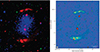 |
Fig. 1. PSZ2 G096.88+24.18. Left: Composite optical (DSS2, green) + radio total intensity (Stokes I, red) + XMM-Newton (blue) image of the cluster. Right: Radio total intensity image obtained with VLA in the L-band (resolution 9.6″ × 9.2″, RMS noise |
Properties of PSZ2 G096.88+24.18 from the literature.
Using optical and X-ray data, Finner et al. (2021) investigated the merger scenario of PSZ2 G096.88+24.18. They estimated a 1:1 mass ratio, with a total mass of  , from simultaneously fitting two Navarro-Frenk-White halos to the lensing signal. Combined with the spectroscopic results of Golovich et al. (2019), who found a single-peak redshift distribution of galaxies associated with PSZ2 G096.88+24.18, the merger is likely a head-on collision on the plane of the sky and the time since collision is
  . The dynamical status of the system is supported by X-ray observations, as the cluster shows two clumps of gas at a projected distance of ∼600 kpc.
de Gasperin et al. (2014) discovered a pair of radio relics on the northern and southern edges of PSZ2 G096.88+24.18 at 1.4 GHz with the Westerbork Synthesis Radio Telescope. The two relics have dimensions of ∼900 kpc (northern) and ∼1.4 Mpc (southern), and are at a distance from the midpoint between the two X-ray peaks of emission of 770 kpc and 1145 kpc, respectively. From a polarization analysis de Gasperin et al. (2014) found that the relic N has electric field vectors mostly aligned perpendicular to the relic extension meaning that the magnetic field is aligned with the relic, with a fractional polarization up to ∼30%. However, the relic S shows vectors that are ∼45° apart from being perpendicular to the relic extension, with a lower polarization fraction that reaches values of about 10%.
Jones et al. (2021) studied this cluster using LOw Frequency ARray (LOFAR, van Haarlem et al. 2013) high band antenna (HBA) observations, at 120–187 MHz, and VLA L-band radio observations (with C and CnB-B configurations), as well as Chandra X-ray observations of the cluster. The morphology, location at the cluster periphery, and spectral index variation of the arc-like radio structures in PSZ2 G096.88+24.18 confirm that we are observing a pair of radio relics. At 144 MHz the relics have largest linear sizes (LLSs) of ∼0.9 and 1.5 Mpc and a flux ratio of 1:3.5 for the north and south relics respectively. Both relics have a nonuniform brightness along their major axis, and high-resolution images show filament-like substructures in the northern relic. Both the north and south relics exhibit spectral steepening from the shock edge toward the cluster center, which is expected from downstream synchrotron and inverse Compton (IC) losses, as this has been observed in many other relics (e.g., Bonafede et al. 2012; van Weeren et al. 2016; Hoang et al. 2017). In their polarimetric analysis, they found that in the northern relic there are significant regions of polarized emission, mostly corresponding to the brightest parts of the relic, with a linear polarization fraction that ranges from 10% to 60% and a magnetic field ordered and compressed along the shock front, as a consequence of the shock passage (Enßlin et al. 1998). The southern relic shows polarized emission in only a few small regions and the polarization fraction is much lower than in the northern relic, reaching a maximum of 20%. In these small regions, the electric field vectors do not lie perpendicular to the shock, in agreement with the results by de Gasperin et al. (2014) although obtained with a different dataset. Despite the availability of X-ray data, they were unable to detect evidence of a shock front at the position of the relics. Due to the low count statistics in the cluster outskirts, the Chandra data are likely not sensitive enough to detect a shock. Finner et al. (2021) also did not detect a shock with a 12 ks XMM-Newton observation. Recently, Tümer et al. (2023) found an indication of a shock front coinciding with the northern relic with Chandra and NuSTAR spectra, but deeper exposures are required to draw more accurate surface brightness profiles that can confirm it.
3. Data analysis
3.1. Calibration
We used both new and archival observations of PSZ2 G096.88+24.18 performed with VLA in the L-band (1–2 GHz). We analyzed a total of 7.5 hours of observations: 4 hours in B-configuration, 3 hours in C-configuration, and 0.5 hours in D-configuration (see also Table 2). With respect to previous studies, which only used C- and CnB-configurations, our observations are sensitive to a broader range of angular scales.
List of the observations used in this paper.
The dataset were preprocessed with the VLA CASA2 (McMullin et al. 2007) calibration pipeline. This pipeline is optimized for Stokes I continuum data and it performs standard flagging and calibration procedures. We used the CASA 5.6.1 package to complete the calibration for the cross-correlation polarization products too and to perform additional flagging. In particular, we used the rflag algorithm, gradually decreasing the flagging threshold from 5σ to 2σ in both time and frequency when necessary. We also applied manual flagging to flag entire spectral windows. We derived final delay, bandpass, gain or phase, leakage, and polarization angle calibrations. We used the Perley & Butler (2013) flux density scale for wide-band observations as a model for the primary calibrator of each observation (3C286). We used as phase calibrators: J1849+6705 (B-Configuration), J2022+6136 (C-configuration), and J1748+7005 (D-configuration). An unpolarized source was used to calibrate the on-axis instrumental leakage (J1407+2827 for B- and D-configurations, and quasi-stellar object B1404+286 for the C-configuration). The primary calibrator was also used for the absolute polarization angle calibration. We made a polynomial fit to its known values of linear polarization fraction and polarization angle to build a frequency-dependent polarization model, following the NRAO polarimetry guide3. The final calibration tables were applied to the target.
Radio frequency interference (RFI) was removed manually and using statistical flagging algorithms also from the cross-correlation products (RL, LR). The calibrated data were then averaged in time down to 10 s and in frequency to the channel width of 4 MHz, in order to speed up the subsequent imaging and self-calibration processes.
3.2. Total intensity imaging
For the total intensity imaging and the self-calibration we used the CASA v6.4.0.16 package. Data were imaged using the tclean task of CASA with the multi-scale, multi-frequency imaging deconvolution algorithms, in order to better reconstruct the extended structure of the source. Moreover, we used three orders in Taylor expansion (setting nterms = 3, Rau & Cornwell 2011) to take into account both the source spectral index and the primary beam response at large distances from the pointing center. Given the wide field to be imaged (∼28′×28′), we also used the w-projection algorithm (Cornwell et al. 2008) to correct for the sky curvature and better clean the most peripheral sources of the image, reducing the artifacts: we imposed wprojplanes = 256. For all the configurations, we used a Briggs weighting scheme (Briggs 1995) with a robustness parameter of 0. For the sole D-configuration, we performed four self-calibration cycles in order to improve the image quality.
Once the different configurations had been inspected individually, we combined the observations in the visibility space, in order to obtain a single dataset over which we would perform our polarimetric analysis. From this final combined dataset, we subtracted the sources outside a region of about a 12′ radius in order to focus only on the cluster region and speed up the computational time in the following analysis. We note that, by restricting the subsequent polarization analysis to the central region of the field, we ensured that the polarization leakage due to instrumental effects is below the 2% level. The final image has a restoring beam of 9.6″ × 9.2″, using a Gaussian taper of 10″, and noise of  (Fig. 1).
4. Polarization analysis
4.1. Polarization imaging
Once our combined dataset had been obtained, we had to prepare the way for the RM synthesis technique. We used WSClean v3.1 (w-stacking clean, Offringa et al. 2014) to produce images in Stokes I, Q, and U. With this software, it is possible to make both a multi-frequency synthesis (MFS) image and a cube with an image made for each channel, required for the RM synthesis using the CIRADA RM-tools v1.2.04 (Purcell et al. 2020). We produced a cube made by 64 images for I, Q, U Stokes, as well as a wide-band image.
We used 64 images for each cube with a bandwidth of 16 MHz per image. This choice was motivated by the fact that, within each channel, we are sensitive to a maximum observable  (see Sect. 4.5): this means that we do not have significant bandwidth depolarization within the channels, since RM in non-cool-core clusters is generally below 5000 rad m−2 (Böhringer et al. 2016). The three Stokes images were cleaned separately, using join-channels for the multi-frequency deconvolution. This performs peak finding in the squared sum over all output channels, but subtracts components independently from the channels. We also used the Briggs weighting scheme with robust = 0. For the imaging cube, we forced all the 64 images to have the same restoring beam, corresponding to the one of the first sub-band (the lowest-resolution one, 13″). We did this also for the MFS images, in order to be consistent in the comparison of the obtained results. Then, the MFS images as well as the I, Q, and U Stokes imaging cubes were corrected for the primary beam (PB). In CASA, we can use the task widebandpbcor in order to compute a set of PBs at the specified frequencies; in our case, 64 PBs, corresponding to the ones that constitute the imaging cubes. Lastly, within the 64 images of the cubes, eight were removed because the frequencies between 1.51 and 1.65 GHz were completely flagged because of the strong RFI. The final PB-corrected cubes are composed of 56 images.
4.2. Integrated polarization results
Before performing the RM synthesis, we decided to evaluate the polarization fraction of the relics integrated over the full band. This would serve as a reference value to evaluate the depolarization due to bandwidth-averaging. To do this, we used the MFS images produced with WSClean and corrected for the PB. We evaluated the integrated flux in P (SP, int) and in total intensity, I (SI, int). We selected two regions, one for each relic, within which we calculated the polarization fraction. These regions were selected following the 5σ contour for both relics in the total intensity image, where σ is the root mean square (RMS) noise of the total intensity image, and are shown in Fig. 2.
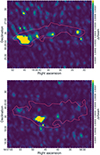 |
Fig. 2. Map of the polarized intensity for each pixel resulting from the RM synthesis, after RM clean (resolution 14″ × 13.2″, RMS |

The polarization image was obtained by combining the Q and U images and then correcting for Ricean bias following George et al. (2012), in which the intrinsic polarized intensity for each pixel is
 (2)
(2)
 is the observed polarized flux, while the value σPobs was computed considering the average RMS noise level between the Qobs and Uobs images and is
  . For each region, the flux density in both total intensity, I (SI, int), and polarized intensity, P (SP, int), was obtained, as well as the respective statistical flux error, calculated as
 (3)
(3)
where flux = I, P, and nbeam is the number of beams within the chosen region. Here, we ignored the systematic error on the flux scale, as we are interested in the relative polarization fraction. The measured flux densities and their uncertainties are listed in Table A.1.
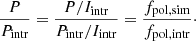
We calculated the integrated polarization fraction for both regions as
 (4)
(4)
and the error on the polarization fraction was obtained through the propagation of errors,
 (5)
(5)
For the selected regions, given the flux densities listed in Table A.1 for I and P, respectively, we obtained the fractional polarization from the integrated analysis, fpol, int, of
(12.1 ± 0.2)% for the north region, and
(5.8 ± 0.1)% for the south region.
These values are compatible with the results obtained by Jones et al. (2021) who found very low levels of fractional polarization for the southern relic (≤10%).
4.3. Depolarization mechanisms
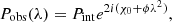
In the presence of a magneto-ionized screen with a homogeneous distribution of thermal electrons and magnetic field, the complex polarized intensity of synchrotron radiation affected by Faraday rotation is
 (6)
(6)
where Pint is the intrinsic polarization of the synchrotron emission, χ0 is the relative intrinsic polarization angle at the source of emission, and ϕ quantifies the Faraday rotation caused by the foreground magneto-ionic medium. However, the observed polarization intensity, Pobs(λ), can be significantly lower with respect to the intrinsic value, Pint, in the presence of more complex Faraday screens. The polarized flux can be reduced by the mixing of different polarization angles along the line of sight. Several instrumental effects can also depolarize the observed radiation. Depolarization toward longer wavelengths can occur due to the mixing of the emitting and rotating media, as well as from the finite spatial resolution of our observations (O’Sullivan et al. 2012). Here, we present the main depolarization mechanisms, following the discussions in Sokoloff et al. (1998) and Stuardi et al. (2022):
-
Differential Faraday rotation: This effect occurs when the emitting and rotating regions are co-spatial and in a regular magnetic field. The polarization plane of the emission at the far side of the region undergoes a different amount of Faraday rotation compared to the polarized emission coming from the near side, causing depolarization when summed over the entire region. For a uniform slab, we have
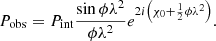 (7)
(7)We note that depolarization increases with wavelength.
-
Internal Faraday dispersion: This occurs when the emitting and rotating regions are co-spatial and contain a turbulent magnetic field. In this case, depolarization occurs because the plane of polarization experiences a random walk through the region. For identical distributions of all the constituents of the magneto-ionic medium along the line of sight, it can be described by
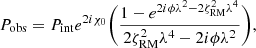 (8)
(8)where ζRM is the internal Faraday dispersion of the medium.
-
External Faraday dispersion/beam depolarization: This occurs in a purely external non-emitting Faraday screen. In the case of turbulent magnetic fields, depolarization occurs when many turbulent cells fall within the synthesized telescope beam. On the other hand, for a regular magnetic field, any variation in the strength or direction of the field within the observing beam will lead to depolarization. Both effects can be described by
 (9)
(9)where σRM is the dispersion about the mean RM across the source on the sky. In this case, the depolarization increases with increasing beam size.
-
Bandwidth depolarization: It occurs when a significant rotation of the polarization angle of the radiation is produced across the observing bandwidth and the polarization fraction is computed averaging over the band.
4.4. Rotation measure synthesis
In this section, we present the basic concepts of the RM synthesis technique, which we used to evaluate the polarized flux of the two radio relics. The RM synthesis allows one to recover the value of the Faraday depth, ϕ (see Eq. 1), and to study the polarized emission from a source. We refer to Brentjens & de Bruyn (2005) for a detailed description of this procedure. The simplest example of Faraday rotation is given by a single source along the line of sight in a uniform rotating medium: in this case, the observed polarization vector can be written as Eq. (6), and the corresponding observed polarization angle is given by
 (10)
(10)
The Faraday depth, ϕ, coincides with the RM when there is no internal Faraday rotation and there is only one source along the line of sight (Brentjens & de Bruyn 2005). As we shall see in Sect. 4.5, this is also the case for the relics studied in this paper.
The RM synthesis allows us to solve for the so-called “nπ ambiguity”, correct for bandwidth depolarization, and recover low signal-to-noise sources. Furthermore, Burn (1966) found a Fourier transform relationship between the observed polarized flux and the polarized flux expressed as a function of the Faraday depth that is still valid when the relationship between χ and λ2 is nonlinear. Brentjens & de Bruyn (2005) extended the work of Burn (1966), introducing a weight function (also known as “window function”), W(λ2), which is nonzero only at values of λ2 that are sampled by the telescope. With this implementation, we can rewrite the observed polarized flux density as
 (11)
(11)
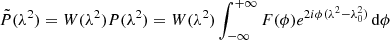
and the “reconstructed” Faraday dispersion function (FDF), also known as “Faraday spectrum” (Fig. 3), as
 |
Fig. 3. RM synthesis results. Top: RMSF for our observations. The dashed orange and dotted green lines represent the real and imaginary components, respectively, while the blue line shows the total amplitude. Bottom: Faraday spectrum for one pixel of the northern relic. We show here both the dirty (dashed blue line) and the cleaned (orange line) spectra. The horizontal red line represents the threshold used for RM clean, and in green we have the clean component selected by the cleaning algorithm. In light red we show the range of ϕ used to evaluate |

 (12)
(12)
where K is the inverse of the integral over W(λ2), ⊛ denotes convolution, and R(ϕ) is the so-called RM transfer function (RMTF) or RM spread function (RMSF, Fig. 3):
 (13)
(13)
In this work, the latter denomination will be used.
The quantity  is the mean of the sampled λ2 values, weighted by W(λ2).
  is F(ϕ) convolved with R(ϕ), and therefore after Fourier filtering by the weight function W(λ2). The quality of reconstruction depends mainly on the weight function W(λ2). Hence, a complete and wide range of λ2 measurements leads to a better defined RMSF and a fine sample in ϕ space, enabling a better reconstruction of F(ϕ). Brentjens & de Bruyn (2005) showed that Eqs. (12) and (13) can be approximated as sums.
Three main parameters are involved when using the RM synthesis technique: the channel width, δλ2, the width of the λ2 distribution, Δλ2, and the shortest wavelength squared,  . These parameters determine, respectively, the maximum observable Faraday depth, the resolution in ϕ space, and the largest scale in ϕ space to which one is sensitive. Given the parameters of our L-band observations, the FWHM of the main peak of the RMSF in our data is given by
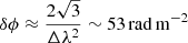 (14)
(14)
the scale in ϕ space to which the sensitivity has dropped to 50% is
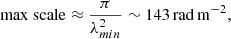 (15)
(15)
and the maximum Faraday depth to which one has more than 50% sensitivity is
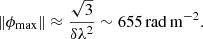 (16)
(16)
The reported numeric values have been obtained for our observations.
4.5. Results of rotation measure synthesis
Besides the integrated analysis of polarization, we applied the RM synthesis technique to resolve the in-band depolarization and understand if the low polarization fraction observed in the southern relic could be due to bandwidth depolarization, as well as to see if there are complex Faraday effects that can also cause depolarization (like the “internal depolarization”, for example). This technique, as was already explained in Sect. 4.4, uses an observing bandwidth split up into many individual narrow frequency channels. Adding up the individual channels may cause bandwidth depolarization; however, using the value of Faraday depth that maximizes the signal resulting from the co-addition of the polarized flux from all channels, it is possible to recover the polarized flux. With the RM synthesis technique, it is possible to obtain the reconstructed Faraday spectrum for each pixel. To perform the RM synthesis technique on image-frequency cubes, we used the RMsynth3D tool present in the RM-tools software. This package takes two input files (Stokes Q and U cubes produced with WSClean) and a list of channel frequencies in order to produce as outputs:
-
The dirty FDF cube (
 ), which represents the polarized flux as a function of the Faraday depth for each pixel, made by two components: the real (Stokes Q(ϕ)) and the imaginary (Stokes U(ϕ)). An example FDF for a single pixel is shown in the bottom panel of Fig. 3.
 -
The RMSF (Fig. 3, top panel), which results from the wavelength coverage and sampling of our observation.
-
A map of the maximum polarized intensity in each FDF (e.g., for each pixel, Fig. 2).
-
A map of the Faraday depth corresponding to the maximum polarized intensity in each FDF.
These last two products were calculated from the Faraday depth values sampled by the FDF, without interpolation over the discrete channels. Moreover, we also provided a list of RMS for each frequency-channel of the cube (σchan, as the average RMS values between Q and U images of each channel) that was used to compute the weight of each frequency channel as the inverse of its RMS, as well as the theoretical noise in P (σP):
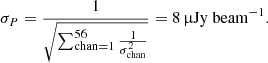 (17)
(17)
The range of Faraday depths over which we calculated the FDF was set to be  , while the sample spacing in Faraday depth for the FDF is
  : the wide range in ϕ for the FDF was chosen in order to use the external intervals to evaluate the noise in each pixel, given that
  . Once we had performed the RM synthesis at 13″, we also “cleaned” the dirty FDF using the FDF deconvolution. This deconvolution is possible using the package RMclean3D, which applies the CLEAN algorithm independently to every pixel in a Faraday depth cube. As a stopping criterion, a cutoff threshold was set to 8σP, following George et al. (2012), which corresponds to a false detection rate of 0.06% and to a Gaussian significance level of about 7σ according to Hales et al. (2012). The cutoff threshold was reached for every pixel for which the RM clean was performed.
To study of the polarization fraction within the two relics, we used the map produced by RMsynth3D showing the maximum polarized intensity in each pixel using cleaned FDF. Then, it was necessary to correct for Ricean bias (Eq. 2). The value  was computed considering the average RMS noise level between the real and imaginary cleaned FDF evaluated in the ranges of
 ![Mathematical equation: $ [-1000,-600]\,\rm{rad\,m^{-2}} $](/articles/aa/full_html/2024/11/aa50892-24/aa50892-24-eq41.gif) and
and ![Mathematical equation: $ [+600,+1000]\,\rm{rad\,m^{-2}} $](/articles/aa/full_html/2024/11/aa50892-24/aa50892-24-eq42.gif) along the Faraday depth axis (Fig. 3, bottom panel).
along the Faraday depth axis (Fig. 3, bottom panel).
With respect to the results obtained with the integrated analysis, owing to the usage of the RM synthesis technique, we detected a higher P than in the integrated analysis (Table A.1). Given the flux densities and respective errors, we obtained a value of fractional polarization, fpol, rm, of
-
(18:6 ± 0:3)Å for the northern region, and
-
(14:6 ± 0:1)Å for the southern region.
These results confirm that bandwidth depolarization has important effects on the polarization fraction of these relics and that we can solve it using the RM synthesis. For the northern region, we obtained a fractional polarization close to the typical value for radio relics (∼20%, Stuardi et al. 2022). However, even if the polarization fraction increases with respect to the integrated analysis, the average polarization fraction of the southern relic remains lower than observed in other relics and in the northern one.
The RM maps of the two relics are shown in Fig. 4 and the distribution of RM values over the relics’ regions is shown in Fig. 5. The RM values have been corrected for the galactic RM (−4.5 rad m−2, from Oppermann et al. 2015). The low values for both relics suggest that we do not have Faraday rotation within the single channels, and so bandwidth depolarization. The average value of RM is slightly larger for the southern relic (−4.5 rad m−2) with respect to the northern one (3.7 rad m−2), but the value of σRM is higher for the northern relic (6.6 rad m−2, against 3.4 rad m−2 for the southern relic): this indicates that the RM is more uniform in the south relic, while it varies more across the northern relic and this, according to Eq. (9), should result in more depolarization. In Fig. 4 we also report the resulting polarization angles, computed using the following Eq. (6) in Stuardi et al. (2019). We point out that the northern relic has E-field vectors oriented mainly perpendicular to the extent of the relic, as expected for such structures (van Weeren et al. 2019), with the exception of a few pixels in the upper part, while the southern relic shows E-field vectors oriented parallel to the relic, confirming the results in de Gasperin et al. (2014).
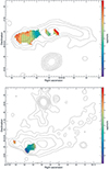 |
Fig. 4. RM map in |

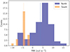 |
Fig. 5. Histograms that show the distribution of RM values for the northern (blue) and southern (orange) relics taken from Fig. 4. The dashed vertical line represents the average RM values of the two relics. The average |

Another result from the RM synthesis is the presence of a small number of pixels that show a complex Faraday spectrum, particularly for the northern relic (see Appendix B for more details). This implies that our assumption of external Faraday rotation could be too simplistic. After the RM clean, which is based on the theoretical noise level, we notice the presence of some pixels that show multiple components. However, after a careful analysis, we found that most of them are below the noise level, which in these cases is larger than the theoretical prediction. Moreover, they are just a small fraction and are not localized in a restricted area but rather scattered, especially at the “border” of the detection. For all these reasons, we believe that they are not necessarily related to complex behaviors in the emitting regions, and that the observed RM is mainly external to the relics.
The results from RM synthesis and the absence of any significant complex Faraday spectrum at our resolution let us conclude that the depolarization has an external nature, related to the gas distribution within the cluster in the direction of the relic.
4.6. Polarization at different resolutions
Under the assumption that the depolarization is external and due to the ICM, we wanted to constrain the magnetic field properties that can reproduce the beam depolarization. To do this, we analyzed how the polarization fraction varies with respect to the beam size. The resolution was changed directly through WSClean, where it was progressively lowered using a Gaussian taper, starting from the 13″ to 50″ for all the 64 images that constitute the Q and U cubes, as well as the Stokes I MFS images. For each resolution we performed an analysis of polarization fraction, following the routine explained in Sections 4.2 and 4.5, for both integrated and RM synthesis technique analysis.
The results for both total intensity (SI) and polarized (SP) flux densities, within the regions selected for the relics, are listed in Table A.1, for the integrated analysis and RM synthesis, respectively. Given the flux densities, following Eqs. (4) and (5), we calculated the trend of polarization fraction as a function of the beam size. The results are listed in Table 3 for integrated and RM synthesis analysis, respectively. The fractional polarization as a function of the resolution is shown in Fig. 6.
Polarization fractions and respective errors measured for the selected regions at different resolutions.
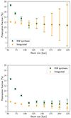 |
Fig. 6. Comparison between the depolarization as a function of beam size evaluated by an integrated analysis (in orange) and using the RM synthesis technique (in green). Top panel: Northern relic. Bottom panel: Southern relic. |
We see that the depolarization decreases with increasing resolution, as is expected for beam depolarization. In particular, comparing the two relics, we notice that the decreasing trend is larger for the southern relic: when we evaluate the difference between the fractional polarization at 13″ (∼58 kpc) and 25″ (∼111 kpc), we find a reduction in the polarization fraction of (64 ± 2)% for the southern relic. For the northern relic, instead, we find a decrease of (42 ± 5)% in the same resolution range. A Kolmogorov-Smirnov test shows a statistically significant difference between the depolarization trends of the two relics (KS statistics of 0.78, p = 0.63%). The plateau that shows up at lower resolutions (beyond 25″, so around 111 kpc on a physical scale) points to the fact that the turbulent magnetic field fluctuations within the beam start to become less significant for large beam sizes. We also notice that the error increases for lower resolutions. This is mainly due to the fact that, recalling Eq. (3), we have a progressively smaller number of beams within the regions that have been used to evaluate the flux. At low resolution, the fractional polarization evaluated with RM synthesis is higher than the integrated one for the southern relic, while the two reach approximately the same values for the northern relic. This may also indicate higher average RM values at low resolution for the southern relic. This trend, which also depends on the magnetic field properties, is what we shall study in the following part of this work, in order to constrain the characteristics of the cluster magnetic field.
5. Comparison to simulations
In this section, we describe the 3D magnetic field simulations made in order to constrain the magnetic field characteristics of PSZ2G096.88+24.18. We simulated magnetic fields with different power spectra and derived the polarization fraction expected for the southern relic at different resolutions. Then, we compared this resolution dependence with the observational results in order to constrain the best-fit magnetic field parameters that reproduce the observed depolarization trend with the beam size.
5.1. Simulation of rotation measure maps
The determination of the cluster magnetic field properties from the RM measurements relies on a the knowledge of both the thermal electron density and the magnetic field structure (see Eq. (1)). In order to avoid simplistic assumptions, often used to solve the integral for ϕ, we produced synthetic RM maps by taking into account 3D models of the thermal electron density and of the magnetic field of a galaxy cluster. These RM maps can then be used to compute depolarization trends that can be compared with observations, where the magnetic field model parameters can be constrained with a statistical approach. This method has been applied in other work to study cluster magnetic fields, as in Bonafede et al. (2011) or Osinga et al. (2022), but to our knowledge it has never been applied to the variation in the polarization fraction with respect to the resolution. This approach can give us additional information on the physical scales on which the magnetic field fluctuates. In order to simulate a distribution of thermal electron density and magnetic field, we used a modified version of the MIRÓ code described in Bonafede et al. (2013) and in Stuardi et al. (2021). We present here the different steps.
The code starts from a mock 3D thermal electron density distribution of a merging cluster. Due to the complexity of the system and the lack of sensitive observations, it was not possible to use a thermal electron density model derived from X-ray data. Hence, we used a merging galaxy cluster analyzed in Domínguez-Fernández et al. (2019) that shares common properties with our observed cluster. It has two density clumps with a projected distance of ∼900 kpc, with a 1:1 mass ratio of the merging sub-clusters. The original simulation had a resolution of 16 kpc at z = 0.02: it was then rescaled in order to have a pixel size of 8 kpc, which is necessary to sample with more than 3 pixels the beam of our highest-resolution observations. This sets the maximum possible wavenumber of the magnetic field power spectrum corresponding to magnetic field fluctuation on the physical scale of 16 kpc. The size of the simulated box is 5123 pixels ( ); therefore, the minimum possible wavenumber corresponds to a physical scale of
  .
.
Then, the code produces a 3D distribution of the magnetic field, based on an analytical power spectrum within a fixed range of scales. In this paper, we used both a simplistic Kolmogorov power-law spectrum (where EB ∝ k−11/3) and a magnetic spectrum derived from Domínguez-Fernández et al. (2019) (in this paper we refer to it as “PDF”),
![Mathematical equation: $$ \begin{aligned} E_{B}(k) = Ak^{3/2} \Biggl [1-\mathrm {erf}\Biggl [B \ln {\Biggl (\frac{k}{C}\Biggr )}\Biggr ]\Biggr ]. \end{aligned} $$](/articles/aa/full_html/2024/11/aa50892-24/aa50892-24-eq48.gif) (18)
(18)
Here  is the wavenumber corresponding to the physical scale of the magnetic field fluctuations (e.g., Λ ∝ 1/k), with i representing its three components. The A parameter gives the normalization of the magnetic spectrum, B is related to the width of the spectra, and C is a characteristic wavenumber corresponding to the inverse outer scale of the magnetic field. The parameters B and C were taken from the E5A simulated cluster in Domínguez-Fernández et al. (2019)5, and have values of B = 1.054 and
 ![Mathematical equation: $ C = 8.708\,k[1/2\,\rm{Mpc}] $](/articles/aa/full_html/2024/11/aa50892-24/aa50892-24-eq50.gif) .
.
In order to obtain a divergence-free turbulent magnetic field with this power spectrum, we first selected the corresponding power spectrum for the vector potential,  , in Fourier space (Murgia et al. 2004; Tribble 1991). For each pixel, in Fourier space, the amplitude, Ak, i (where i represent its three components), was taken from a Rayleigh distribution in order to have magnetic field components that follow a Gaussian distribution, and the phase of each component of
  was randomly drawn in the range [0, 2π]. The magnetic field vector in Fourier space is then
  and has the desired power spectrum.
  was transformed back into real space using an inverse fast Fourier transform (FFT) algorithm. The resulting magnetic field, B, has components, Bi, following a Gaussian distribution, with ⟨Bi⟩ = 0 and
  .
.
The radial profile of the magnitude of the magnetic field is expected to scale with the thermal electron density. This radial decrease in the magnetic field strength is also expected by MHD simulations (e.g., Vazza et al. 2018; Domínguez-Fernández et al. 2019). Therefore, we imposed that the cluster magnetic field scales with the thermal electron density, following a power law,
 (19)
(19)
where η was set at 0.5, obtained in Bonafede et al. (2010), which we expect if the energy in the magnetic field scales as the energy in the thermal plasma (assumed to be isothermal).
The magnetic field was scaled by the density profile and then normalized for a value, Bmean, over the entire box. Hence, the generated cluster magnetic field is tangled on both small and large scales, and it decreases with the thermal electron density. In the case of the PDF power spectrum, Bmean also set the A parameter of the analytical formula in Eq. (18). Bmean was chosen in order to give, at the southern relic position, a magnetic field equal to the one evaluated with the equipartition assumptions. Following Eq. (26) in Govoni & Feretti (2004), we find an equipartition magnetic field of  6. The value of Bmean that gives us the equipartition value at the southern relic position is
  , so we decided to fix this value in order to limit the number of free parameters for the simulations.
Finally, the code computed the cluster 2D RM map integrating the thermal electron density and magnetic field profile along one axis, solving Eq. (1), from the center of the cluster, and thus assuming that the sources lie on the plane parallel to the plane of the sky and crossing the cluster center.
To summarize, we fixed the following parameters for the simulations: the size and resolution of the box, the parameter η, the factors, B and C, of the PDF magnetic field power spectrum, and the normalization factor, Bmean. The only free parameters are the minimum and maximum scale over which the magnetic field power spectrum is defined.
5.2. Simulated polarization fraction
For the simulation of the polarization fraction at different resolutions, we used the 2D RM maps produced by the MIRÓ code. To compute the depolarization effect for different magnetic field models, we used an approach similar to the one used in Osinga et al. (2022)7. For the simulated fractional polarization, we have to assume an intrinsic polarization vector for each pixel in our simulated RM map. We assumed a uniform distribution, with χ0 = 45°. The choice of the intrinsic polarization angle is arbitrary, while the uniform distribution is driven by the assumption that intrinsic polarization vectors are all aligned by the shock passage. We also assumed an intrinsic polarized flux density of  for each pixel. This was an arbitrary choice since we are only interested in the change of polarization with the beam size, P/Pintr, where P is the polarized flux measured after smoothing.
Once we have obtained χ with Faraday rotation using the simulated RM map ( ), and using P, we can compute the Stokes Q and U parameters using the following relations:
 (20)
(20)
which we can convert to
 (21)
(21)
using the convention that Stokes Q is positive for −π/2 ≤ χ ≤ π/2 and Stokes U is positive for 0 ≤ χ ≤ π. The Q and U simulated images were smoothed with a Gaussian kernel with dimensions equal to the ones used to trace the observed depolarization trend, and the smoothed P was computed again using Eq. (20). Finally, we generated the maps of P/Pintr at different resolutions (an example is shown in Fig. 7).
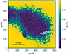 |
Fig. 7. 2D smoothed map at 13″ of polarized intensity over intrinsic polarized intensity, resulting from the depolarization code presented in Osinga et al. (2022). In white, we highlight the region chosen to extract the simulated polarization fraction for the southern relic. |
From the simulations, we obtained P/Pintr, which is the loss of polarization intensity due to Faraday rotation at different resolutions and not the polarization fraction that we measure from observations. Thus, we needed to rescale it to compare the data and the model:
 (22)
(22)
This means that we have a relationship between the simulated and the intrinsic polarization fraction, which is:
 (23)
(23)
Given that we do not know the intrinsic polarization fraction, we used an assumption based on Enßlin et al. (1998). According to their formalism, if the magnetic pressure of the relics is small compared to the internal gas pressure, the compression of the magnetized regions is equal to the compression of the accretion shocks. If we use the values related to the southern relic8, gives a fpol, intr ∼ 54.7% (using Eq. (22) in Enßlin et al. 1998). We assume this as the intrinsic polarization fraction fpol, int. This means that we have to scale our simulation by this value, given the Eq. (23), in order to obtain the simulated polarization fraction, that we need to compare the data and models. We selected a region in the simulated polarization maps (highlighted as white boxes in Fig. 7) with the same position and dimensions as the southern relic (as reported in Finner et al. 2021; Jones et al. 2021). Within this region, we evaluated the polarization fraction for the southern relic at different resolutions, matching those in our observations.
5.3. Data and simulations comparison
To compare the data and simulations, and assess which magnetic field power spectrum better reproduces the observed depolarization trend, we used a reduced chi-squared test that takes into account the error on the observed polarization fraction, as well as the observed and simulated ones. To consider the statistical fluctuations related to the simulations, we made a set of ten runs for each magnetic field power spectrum, with a certain combination of minimum and maximum scales. Then, we averaged the values obtained at each resolution in order to get an average trend, taking into account all the simulation runs, and this average trend was then compared with the observed data using the reduced chi-squared test,
 (24)
(24)
This evaluation of the reduced chi-squared comes from Govoni et al. (2006), where i represents the nine resolutions used for the beam size, Oi are the observed data, ⟨Ci⟩10 represents the simulated data averaged over the ten identical runs of simulations for any combination of scales, δfpol, rm i represents the error on the observed data, and  represents the standard deviation of the simulations.
We only varied the scales, Λmin and Λmax, over which the magnetic field power spectrum was defined. The minimum scale of 16 kpc was limited by our observational capabilities, while for the maximum scale we were limited by the size of the problem, because we wanted to execute and replicate the simulations multiple times within acceptable run-times. We expect Λmin below 16 kpc not only from theory (Brunetti & Jones 2014), but also from the fact that at 13″ resolution we already observe depolarization with respect to the expected intrinsic one for the relic (∼54.7% from Enßlin et al. 1998). On the contrary, given the plateau observed over 100 kpc in Fig. 6, we do not expect significantly higher Λmax; otherwise, we should have observed additional depolarization toward larger beam sizes. Once these boundaries for the possible minimum and maximum scales had been defined, we performed multiple simulations, varying the combination of scales.
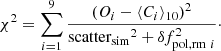
The results of the comparison between data and simulations are represented in Fig. 8, in which we show, for each combination of minimum and maximum scales, the value of the reduced chi-squared on a different color scale. It is important to underline that the ones in the figure represent just a small subsample of all the scales that we used: we just represent these because they surround the best-fit combination of scales. For the Kolmogorov magnetic field power spectrum, we find that the combination of minimum and maximum scales that minimize the reduced chi-squared is  and
and  : this results in
  . For the PDF power spectrum, instead, we find the best fit for a minimum scale of
  and a maximum scale of
  : this gives a reduced chi-squared value of
  .
.
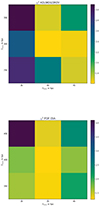 |
Fig. 8. Comparison between the reduced chi-squared values obtained for the two magnetic field power spectra selected for this work. The two axes represent the minimum and maximum scales in kpc over which the spectra were defined. On a color scale, we have the reduced chi-squared evaluated following Eq. (24). Top panel: For the Kolmogorov power spectrum. Bottom panel: For the PDF power spectrum. |
Together with the magnetic field generated by MIRÓ, we also performed the same analysis using the 3D magnetic field directly originated by the MHD simulations in Domínguez-Fernández et al. (2019, E5A cluster). The resulting depolarization trend does not reproduce the observed one: using the magnetic field from the MHD simulation, we obtained a depolarization trend with a higher normalization and a shallower reduction of polarization fraction with increasing beam size (Fig. 9). This results in a reduced chi-squared of  . Comparing the average magnetic field computed at the relic position, we find a value for the MHD simulations a factor ∼3 smaller with respect to the one we imposed with MIRÓ to match the equipartition value (Sect. 5). The higher polarization fraction is thus consistent with the lower magnetic field intensity of the MHD field. The different depolarization trend suggests that the MHD field has a more complex distribution than the one generated by MIRÓ, in which we have also increased the resolution, introducing a fluctuation on smaller scales.
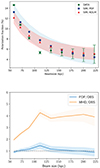 |
Fig. 9. Comparison between observed and simulated polarization trends with beam size. Top panel: Observed depolarization trend with the beam size (green circles) compared with the best-fit models for both the Kolmogorov (red triangles) and PDF (blue squares) magnetic field power spectrum (Sect. 5.3) Bottom panel: Comparison between the simulated depolarization trends normalized for the observed one. The best-fit PDF magnetic field power spectrum found in Sect. 5.3 is in blue, while the magnetic field from MHD simulations is in orange. The dashed, horizontal gray line represents the perfect coincidence between simulation and observational trends. |
6. Discussion
6.1. Origin of the low polarization fraction of the southern relic
In this work, we wanted to study the nature of the low polarization fraction observed in the southern relic of PSZ2 G096.88+24.18 compared to the northern relic using RM synthesis. The origin of the different behavior of polarization in the two relics is not yet understood, and has been investigated in previous work.
de Gasperin et al. (2014) suggested that this could be caused by the southern relic lying further away from us compared to the northern relic. In this scenario, the observed radio emission would have to pass through more magnetized, ionized plasma and would therefore be subject to more Faraday rotation. Spectroscopic observations of PSZ2 G096.88+24.18 show that the redshift distribution of the member galaxies is well fit by a single Gaussian (Golovich et al. 2019). This makes it unlikely that significant additional Faraday rotation due to projection effects is causing the observed difference in polarization angle. However, we need to consider that gas and galaxies can have a different distribution.
The localized nature of the polarized emission and unexpected electric field vector orientation could instead indicate that we are observing emission from a polarized radio galaxy in projection within the relic. Jones et al. (2021) claimed that no optical counterpart was observed and the polarized emission coincides with the brightest part of the relic. However, comparing our radio data with a deep optical image (Fig. 10), we notice the presence of three possible contaminating sources that could contribute to the polarization of the southern relic. Therefore, we cannot exclude the contribution of background sources, even if, given their generally low polarization fraction (below 10%) and the fact that we evaluate the fractional polarization using flux density taken over the whole relic extension, we can conclude that the observed polarization level can only be reached with the contribution of the polarized emission from the relic.
 |
Fig. 10. Total intensity radio contours (same as in Fig. 1) overlaid on a Subaru/Suprime-Cam image of the cluster. We notice that, corresponding to one of the brightest parts of the southern relic, we have possible contaminating background sources that could contribute to the relic polarization. |
Another possible reason for the lack of polarized emission in the southern relic could be that the turbulence in the relic has mixed the magnetic field lines. Turbulence mixes field lines at scales larger than the Alfvén scale (lA), the scale at which the velocity of turbulence is equal to the Alfvén speed (Brunetti & Lazarian 2016). If this scale were smaller than the beam size, then we would observe depolarization effects. In view of this, the stark differences between the northern and southern relics may be explained if the turbulence in the north relic is generated with lower efficiency, or at larger scales than in the southern relic, or has been already partly dissipated.
In Section 4.5, we presented the results obtained with new observations and techniques. With our analysis, we found an increase in the polarization fraction for the southern relic (∼14.6%) with respect to what was found in previous work (values below the 10%, Jones et al. 2021). This is still below the average reported for such systems (Stuardi et al. 2022, ∼20%), and also below the polarization of the northern relic. The RM synthesis is able to solve for the bandwidth depolarization. Given the absence of systematic and significant pixels that show complex Faraday spectra (see Appendix B), we infer that the depolarization of the southern relic has an external nature, related to the properties of the magnetized ICM that is crossed by the relic emission. Unfortunately, the complex morphology of the X-ray emission, together with the low count statistics (Finner et al. 2021; Tümer et al. 2023), does not allow us to reconstruct the density distribution of the thermal gas within the cluster, which is crucial to quantify the effect of the Faraday rotation as well as to recover information on the magnetic field along the line of sight (Eq. (1)). Another important factor that could determine a difference in the polarization properties between the two relics is their 3D position within the cluster. What we observe is the projection of the relics on the plane of the sky but they present a rather complex morphology (Wittor et al. 2019), so variations in RM can be addressed to the fact that different parts of the relic can be at different distances within the cluster, and so the radiation crosses different lengths of the ICM. Given the lack of detailed information currently available on the gas distribution and the inability to get geometric hints from observations, we cannot distinguish clearly the contribution of the two scenarios just discussed to the relic depolarization. Based on the results of our RM study with respect to previous papers, we can discard the hypothesis (raised in de Gasperin et al. 2014) that the southern relic lies further from us, at least for what concerns the portion of the relic observed in polarization. Nevertheless, we cannot exclude that the southern relic is a more complex system, with some parts that, being located deeper in the ICM, are completely depolarized at 13″. From the resulting values of RM, similar between the two relics, and the depolarization trend observed for the southern relic, we favor a scenario in which the southern relic is morphologically more complex and/or located in a more turbulent region of the cluster.
6.2. Constraints on the magnetic field of the cluster
After discussing the origin of the depolarization for the southern relic, we used the beam depolarization to get constraints on the magnetic field distribution within the cluster. This strategy has already been adopted in other papers (Bonafede et al. 2011; Osinga et al. 2022). When synchrotron emission arising from a cluster or background source crosses the ICM, regions with similar intrinsic polarization angles, going through different paths, will be subject to differential Faraday rotation. If the magnetic field in the foreground screen is tangled on scales much smaller than the observing beam, then radiation with similar ϕ but the opposite sign will be averaged out, and the observed degree of polarization will be reduced.
We reproduced the observed beam depolarization trend for the southern relic with simulations of the cluster magnetic power spectrum. This, as was already stated, relies on several assumptions, mainly due to the fact that we do not know the true ICM distribution as well as the true relic structure, which directly affects the computation of the equipartition magnetic field. The equipartition magnetic field computed for the southern relic has been used as a reference to set Bmean for the simulations. From the comparison between the data and simulations shown in Fig. 9, we clearly see that the Kolmogorov power spectrum is not able to reproduce both the normalization of the highest-resolution point and the fast depolarization before reaching the plateau at low resolutions. Moreover, the value of polarization fraction evaluated at 25″ is not fit by any model used for the magnetic field spectrum. Overall, the PDF power spectrum, based on cosmological simulations, is the one that best fits the observed beam depolarization for the S relic. Among the wide range of scales tested, we found that the best combination of minimum and maximum scale is  and
and  , with Bmean set to
  : this results in an average magnetic field over 1 Mpc of
  .
.
7. Conclusions
In this paper, we have addressed the origin of the low fractional polarization that characterizes the southern relic of PSZ2 G096.88+24.18, a galaxy cluster hosting a double radio relic. While the northern relic shows a rather common behavior compared to other radio relics (both in terms of fractional polarization and orientation of the magnetic field lines), the southern relic shows a lack of polarization, as has already been reported in previous works (de Gasperin et al. 2014; Jones et al. 2021), as well as an opposite orientation of the magnetic field vectors with respect to what is expected in the presence of a shock (van Weeren et al. 2019). We used new and archival VLA observations in L-band, using multiple configurations, in order to achieve both high angular resolution and sensitivity to the extended emission. We analyzed the integrated polarization fraction of both relics and we confirmed the low fractional polarization that characterizes the southern relic. To correct for bandwidth depolarization, we used the RM synthesis technique for the polarization analysis. With this technique, we found higher values of fractional polarization for both relics (18.6% for the northern relic and 14.6% for the southern one), yet the southern relic shows lower fractional polarization with respect to the northern one. The two relics show different depolarization trends with increasing beam size, with the southern relic being the one with the greater decrease in polarization fraction. In this RM study, we have also inferred a higher average value of RM for the southern relic with respect to the northern one, which however has a higher σRM: this means that the RM is more uniform in the southern relic. This result also depends on the fact that we detected RM in only a few pixels, and mostly for the northern relic.
We infer that the depolarization has an external nature, related to the different composition or different distribution of the Faraday screen, other than the true structure and position of the relics within the cluster. Unfortunately, given the complexity of the X-ray emission from the ICM, its density distribution has not been determined yet, so we do not have a direct estimate for ne, which is crucial to recover information on the magnetic field along the line of sight (Eq. 1).
We also constrained the magnetic field power spectrum within the cluster using the beam depolarization observed for the S relic. Computing the fractional polarization trend with respect to the beam size with different models, we found that the best combination of parameters that could fit the observations is given by the magnetic field power spectrum presented in Domínguez-Fernández et al. (2019), defined on scales  and
and  . This yields a magnetic field averaged over 1 Mpc scale of
  , which is in line with what is typically found in other clusters, using the Faraday rotation effect for similar studies (Murgia et al. 2004; Bonafede et al. 2010; Stuardi et al. 2022).
M500(200) is the mass enclosed within the radius r500(200), within which the mean density of the cluster is 500(200) times the critical density of the Universe at the cluster redshift.
See Table 1 of Domínguez-Fernández et al. (2019).
Assuming a depth intermediate between length and height, a radio brightness at of  with an α = 1.17 (values taken from Jones et al. 2021), k = 1 as a parameter describing the nature of the plasma (typical value for galaxy clusters), and ξ(α, ν1, ν2) = 3.42 × 10⁻¹³ (as listed in Table 1 in Govoni & Feretti 2004).
α = 0.97 (γ = 2α + 1; Jones et al. 2021), δ = 90°, R = (α + 1)/(α − 1/2).
Acknowledgments
We would like to thank our anonymous referee for the useful comments on this manuscript. We thank A. Botteon for sharing the X-ray data shown in Fig. 1. This paper is supported by the Fondazione ICSC, Spoke 3 Astrophysics and Cosmos Observations. National Recovery and Resilience Plan (Piano Nazionale di Ripresa e Resilienza, PNRR) Project ID CN_00000013 “Italian Research Center for High-Performance Computing, Big Data and Quantum Computing” funded by MUR Missione 4 Componente 2 Investimento 1.4: Potenziamento strutture di ricerca e creazione di “campioni nazionali di R&S (M4C2-19)” – Next Generation EU (NGEU). AB acknowledges support from the ERC-Stg DRANOEL n. 714245. FV has been supported by Fondazione Cariplo and Fondazione CDP, through grant n. Rif: 2022-2088 CUP J33C22004310003 for “BREAKTHRU” project. FdG acknowledges support from the ERC Consolidator Grant ULU 101086378. RJvW acknowledges support from the ERC Starting Grant ClusterWeb 804208. The National Radio Astronomy Observatory is a facility of the National Science Foundation operated under cooperative agreement by Associated Universities, Inc.
References
- Akamatsu, H., & Kawahara, H. 2013, PASJ, 65, 16 [NASA ADS] [CrossRef] [Google Scholar]
- Böhringer, H., Chon, G., & Kronberg, P. P. 2016, A&A, 596, A22 [NASA ADS] [CrossRef] [EDP Sciences] [Google Scholar]
- Bonafede, A., Feretti, L., Murgia, M., et al. 2010, A&A, 513, A30 [NASA ADS] [CrossRef] [EDP Sciences] [Google Scholar]
- Bonafede, A., Govoni, F., Feretti, L., et al. 2011, A&A, 530, A24 [CrossRef] [EDP Sciences] [Google Scholar]
- Bonafede, A., Brüggen, M., van Weeren, R., et al. 2012, MNRAS, 426, 40 [Google Scholar]
- Bonafede, A., Vazza, F., Brüggen, M., et al. 2013, MNRAS, 433, 3208 [NASA ADS] [CrossRef] [Google Scholar]
- Botteon, A., Brunetti, G., Ryu, D., & Roh, S. 2020, A&A, 634, A64 [NASA ADS] [CrossRef] [EDP Sciences] [Google Scholar]
- Brentjens, M. A., & de Bruyn, A. G. 2005, A&A, 441, 1217 [NASA ADS] [CrossRef] [EDP Sciences] [Google Scholar]
- Briggs, D. S. 1995, Ph.D. Thesis, New Mexico Institute of Mining and Technology, USA [Google Scholar]
- Brüggen, M. 2013, Astron. Nachr., 334, 543 [NASA ADS] [CrossRef] [Google Scholar]
- Brunetti, G., & Jones, T. W. 2014, Int. J. Mod. Phys. D, 23, 1430007 [Google Scholar]
- Brunetti, G., & Lazarian, A. 2016, MNRAS, 458, 2584 [Google Scholar]
- Burn, B. J. 1966, MNRAS, 133, 67 [Google Scholar]
- Cornwell, T. J., Golap, K., & Bhatnagar, S. 2008, IEEE J. Sel. Top. Signal Process., 2, 647 [Google Scholar]
- de Gasperin, F., van Weeren, R. J., Brüggen, M., et al. 2014, MNRAS, 444, 3130 [NASA ADS] [CrossRef] [Google Scholar]
- de Gasperin, F., Rudnick, L., Finoguenov, A., et al. 2022, A&A, 659, A146 [NASA ADS] [CrossRef] [EDP Sciences] [Google Scholar]
- Di Gennaro, G., van Weeren, R. J., Rudnick, L., et al. 2021, ApJ, 911, 3 [NASA ADS] [CrossRef] [Google Scholar]
- Domínguez-Fernández, P., Vazza, F., Brüggen, M., & Brunetti, G. 2019, MNRAS, 486, 623 [Google Scholar]
- Enßlin, T. A., Biermann, P. L., Klein, U., & Kohle, S. 1998, A&A, 332, 395 [Google Scholar]
- Feretti, L., Giovannini, G., Govoni, F., & Murgia, M. 2012, A&ARv, 20, 54 [Google Scholar]
- Finner, K., HyeongHan, K., Jee, M. J., et al. 2021, ApJ, 918, 72 [NASA ADS] [CrossRef] [Google Scholar]
- George, S. J., Stil, J. M., & Keller, B. W. 2012, PASA, 29, 214 [Google Scholar]
- Golovich, N., Dawson, W. A., Wittman, D. M., et al. 2019, ApJS, 240, 39 [NASA ADS] [CrossRef] [Google Scholar]
- Govoni, F., & Feretti, L. 2004, Int. J. Mod. Phys. D, 13, 1549 [Google Scholar]
- Govoni, F., Murgia, M., Feretti, L., et al. 2006, A&A, 460, 425 [NASA ADS] [CrossRef] [EDP Sciences] [Google Scholar]
- Hales, C. A., Gaensler, B. M., Norris, R. P., & Middelberg, E. 2012, MNRAS, 424, 2160 [NASA ADS] [CrossRef] [Google Scholar]
- Hoang, D. N., Shimwell, T. W., Stroe, A., et al. 2017, MNRAS, 471, 1107 [Google Scholar]
- Jones, A., de Gasperin, F., Cuciti, V., et al. 2021, MNRAS, 505, 4762 [NASA ADS] [CrossRef] [Google Scholar]
- McMullin, J. P., Waters, B., Schiebel, D., Young, W., & Golap, K. 2007, ASP Conf. Ser., 376, 127 [Google Scholar]
- Murgia, M., Govoni, F., Feretti, L., et al. 2004, A&A, 424, 429 [NASA ADS] [CrossRef] [EDP Sciences] [Google Scholar]
- Offringa, A. R., McKinley, B., Hurley-Walker, N., et al. 2014, MNRAS, 444, 606 [Google Scholar]
- Oppermann, N., Junklewitz, H., Greiner, M., et al. 2015, A&A, 575, A118 [NASA ADS] [CrossRef] [EDP Sciences] [Google Scholar]
- Osinga, E., van Weeren, R. J., Andrade-Santos, F., et al. 2022, A&A, 665, A71 [NASA ADS] [CrossRef] [EDP Sciences] [Google Scholar]
- O’Sullivan, S. P., Brown, S., Robishaw, T., et al. 2012, MNRAS, 421, 3300 [CrossRef] [Google Scholar]
- Perley, R. A., & Butler, B. J. 2013, ApJS, 206, 16 [Google Scholar]
- Planck Collaboration VIII. 2011, A&A, 536, A8 [NASA ADS] [CrossRef] [EDP Sciences] [Google Scholar]
- Planck Collaboration XXVII. 2016, A&A, 594, A27 [NASA ADS] [CrossRef] [EDP Sciences] [Google Scholar]
- Purcell, C. R., Van Eck, C. L., West, J., Sun, X. H., & Gaensler, B. M. 2020, Astrophysics Source Code Library [record ascl:2005.003] [Google Scholar]
- Rajpurohit, K., van Weeren, R. J., Hoeft, M., et al. 2022, ApJ, 927, 80 [NASA ADS] [CrossRef] [Google Scholar]
- Rau, U., & Cornwell, T. J. 2011, A&A, 532, A71 [NASA ADS] [CrossRef] [EDP Sciences] [Google Scholar]
- Rincon, F. 2019, J. Plasma Phys., 85, 205850401 [NASA ADS] [CrossRef] [Google Scholar]
- Sokoloff, D. D., Bykov, A. A., Shukurov, A., et al. 1998, MNRAS, 299, 189 [Google Scholar]
- Stuardi, C., Bonafede, A., Wittor, D., et al. 2019, MNRAS, 489, 3905 [NASA ADS] [Google Scholar]
- Stuardi, C., Bonafede, A., Lovisari, L., et al. 2021, MNRAS, 502, 2518 [NASA ADS] [CrossRef] [Google Scholar]
- Stuardi, C., Bonafede, A., Rajpurohit, K., et al. 2022, A&A, 666, A8 [Google Scholar]
- Tribble, P. C. 1991, MNRAS, 253, 147 [NASA ADS] [Google Scholar]
- Tümer, A., Wik, D. R., Schellenberger, G., Miller, E. D., & Bautz, M. W. 2023, ArXiv e-prints [arXiv:2312.06020] [Google Scholar]
- Vacca, V., Murgia, M., Govoni, F., et al. 2018, Galaxies, 6, 142 [NASA ADS] [CrossRef] [Google Scholar]
- van Haarlem, M. P., Wise, M. W., Gunst, A. W., et al. 2013, A&A, 556, A2 [NASA ADS] [CrossRef] [EDP Sciences] [Google Scholar]
- van Weeren, R. J., Röttgering, H. J. A., Brüggen, M., & Hoeft, M. 2010, Science, 330, 347 [Google Scholar]
- van Weeren, R. J., Brunetti, G., Brüggen, M., et al. 2016, ApJ, 818, 204 [Google Scholar]
- van Weeren, R. J., de Gasperin, F., Akamatsu, H., et al. 2019, ArXiv e-prints [arXiv:1901.04496] [Google Scholar]
- Vazza, F., Brunetti, G., Brüggen, M., & Bonafede, A. 2018, MNRAS, 474, 1672 [NASA ADS] [CrossRef] [Google Scholar]
- Wittor, D., Vazza, F., & Brüggen, M. 2017, MNRAS, 464, 4448 [NASA ADS] [CrossRef] [Google Scholar]
- Wittor, D., Hoeft, M., Vazza, F., Brüggen, M., & Domínguez-Fernández, P. 2019, MNRAS, 490, 3987 [Google Scholar]
- Zwicky, F., Herzog, E., Wild, P., Karpowicz, M., & Kowal, C. T. 1961, Catalogue of Galaxies and of Clusters of Galaxies (Pasadena: California Institute of Technology) [Google Scholar]
Appendix A: Flux density for the beam depolarization
Integrated and RM synthesis polarized flux densities and relative errors measured for the selected regions: north (top) and south (bottom).
Appendix B: Analysis and discussion on the nature of complex Faraday spectra
With the RM synthesis it is possible to obtain the reconstructed (and eventually cleaned) FDF, also called Faraday spectrum, that shows for each pixel the trend of polarized flux as a function of the Faraday depth. In the simplest case in which we observe a source with an intrinsic rotation measure whose radiation crosses a non-emitting magnetized plasma, we expect to observe a  with a single peak, corresponding to the resulting RM value. A good example of this case is represented in Fig. 3. However, there can be some pixels in which the reconstructed FDF shows multiple peaks: this can happen, for example, when several contributions mixes along the same line of sight (e.g., a linearly polarized source whose radiation crosses an emitting magnetized plasma, or the alignment of multiple polarized emitting sources), and in these cases the correct reconstruction of the true RM value can be challenging. We usually point out to these as complex Faraday spectra.
Through our RM synthesis analysis of the relics, we found several pixels (about 6%) showing a complex Faraday spectrum, especially for the north relic. Some examples are shown in Fig. B.1. Usually the presence of such behavior in FDF could mean that there are several contribution to the observed RM along the same line of sight, and so the assumption that we only have a non-emitting Faraday screen would not be valid. However, analyzing all the complex pixels, we notice that they are mainly located at the boundary of the regions selected for the relics and, moreover, they are predominantly dominated by noise. Because of these evidences, we can conclude that they are not to be taken into account for further analysis about their complex topology, that would imply additional features for the reconstruction of the correct RM value.
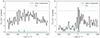 |
Fig. B.1. Example of complex Faraday spectrum for three pixels. The black solid line represents the trend of the cleaned, reconstructed FDF as a function of the Faraday depth ϕ. The horizontal blue dotted line represents the threshold used to select the clean components for the RMclean3D of 8σP (in blue), with |
All Tables
Polarization fractions and respective errors measured for the selected regions at different resolutions.
Integrated and RM synthesis polarized flux densities and relative errors measured for the selected regions: north (top) and south (bottom).
All Figures
|
Fig. 1. PSZ2 G096.88+24.18. Left: Composite optical (DSS2, green) + radio total intensity (Stokes I, red) + XMM-Newton (blue) image of the cluster. Right: Radio total intensity image obtained with VLA in the L-band (resolution 9.6″ × 9.2″, RMS noise |
| In the text | |
|
Fig. 2. Map of the polarized intensity for each pixel resulting from the RM synthesis, after RM clean (resolution 14″ × 13.2″, RMS |
| In the text | |
|
Fig. 3. RM synthesis results. Top: RMSF for our observations. The dashed orange and dotted green lines represent the real and imaginary components, respectively, while the blue line shows the total amplitude. Bottom: Faraday spectrum for one pixel of the northern relic. We show here both the dirty (dashed blue line) and the cleaned (orange line) spectra. The horizontal red line represents the threshold used for RM clean, and in green we have the clean component selected by the cleaning algorithm. In light red we show the range of ϕ used to evaluate |
| In the text | |
|
Fig. 4. RM map in |
| In the text | |
|
Fig. 5. Histograms that show the distribution of RM values for the northern (blue) and southern (orange) relics taken from Fig. 4. The dashed vertical line represents the average RM values of the two relics. The average |
| In the text | |
|
Fig. 6. Comparison between the depolarization as a function of beam size evaluated by an integrated analysis (in orange) and using the RM synthesis technique (in green). Top panel: Northern relic. Bottom panel: Southern relic. |
| In the text | |
|
Fig. 7. 2D smoothed map at 13″ of polarized intensity over intrinsic polarized intensity, resulting from the depolarization code presented in Osinga et al. (2022). In white, we highlight the region chosen to extract the simulated polarization fraction for the southern relic. |
| In the text | |
|
Fig. 8. Comparison between the reduced chi-squared values obtained for the two magnetic field power spectra selected for this work. The two axes represent the minimum and maximum scales in kpc over which the spectra were defined. On a color scale, we have the reduced chi-squared evaluated following Eq. (24). Top panel: For the Kolmogorov power spectrum. Bottom panel: For the PDF power spectrum. |
| In the text | |
|
Fig. 9. Comparison between observed and simulated polarization trends with beam size. Top panel: Observed depolarization trend with the beam size (green circles) compared with the best-fit models for both the Kolmogorov (red triangles) and PDF (blue squares) magnetic field power spectrum (Sect. 5.3) Bottom panel: Comparison between the simulated depolarization trends normalized for the observed one. The best-fit PDF magnetic field power spectrum found in Sect. 5.3 is in blue, while the magnetic field from MHD simulations is in orange. The dashed, horizontal gray line represents the perfect coincidence between simulation and observational trends. |
| In the text | |
|
Fig. 10. Total intensity radio contours (same as in Fig. 1) overlaid on a Subaru/Suprime-Cam image of the cluster. We notice that, corresponding to one of the brightest parts of the southern relic, we have possible contaminating background sources that could contribute to the relic polarization. |
| In the text | |
|
Fig. B.1. Example of complex Faraday spectrum for three pixels. The black solid line represents the trend of the cleaned, reconstructed FDF as a function of the Faraday depth ϕ. The horizontal blue dotted line represents the threshold used to select the clean components for the RMclean3D of 8σP (in blue), with |
| In the text | |
Current usage metrics show cumulative count of Article Views (full-text article views including HTML views, PDF and ePub downloads, according to the available data) and Abstracts Views on Vision4Press platform.
Data correspond to usage on the plateform after 2015. The current usage metrics is available 48-96 hours after online publication and is updated daily on week days.
Initial download of the metrics may take a while.