| Issue |
A&A
Volume 691, November 2024
|
|
|---|---|---|
| Article Number | A64 | |
| Number of page(s) | 15 | |
| Section | Planets and planetary systems | |
| DOI | https://doi.org/10.1051/0004-6361/202450881 | |
| Published online | 30 October 2024 | |
ExoplaNeT accRetion mOnitoring sPectroscopic surveY (ENTROPY)
I. Evidence for magnetospheric accretion in the young isolated planetary-mass object 2MASS J11151597+1937266★
1
Institutionen för astronomi, Stockholms universitet,
AlbaNova universitetscentrum,
106 91,
Stockholm,
Sweden
2
Univ. Grenoble Alpes, CNRS, IPAG,
38000
Grenoble,
France
3
Institute for Advanced Study, Tsinghua University,
Beijing
100084,
PR China
4
Department of Astronomy, Tsinghua University,
Beijing
100084,
PR China
5
Department of Earth and Planetary Science, The University of Tokyo,
7-3-1 Hongo, Bunkyo-ku,
Tokyo
113-0033,
Japan
6
Max-Planck-Institut für Astronomie,
Königstuhl 17,
69117
Heidelberg,
Germany
7
Fakultät für Physik, Universität Duisburg–Essen,
Lotharstraße 1,
47057
Duisburg,
Germany
8
Institut für Astronomie und Astrophysik, Universität Tübingen,
Auf der Morgenstelle 10,
72076
Tübingen,
Germany
9
Physikalisches Institut, Universität Bern,
Gesellschaftsstr. 6,
3012
Bern,
Switzerland
10
ETH Zürich, Department of Physics,
Wolfgang-Pauli-Str. 27,
CH-8093,
Zürich,
Switzerland
11
Department of Astronomy, University of Michigan,
323 West Hall, 1085 South University Avenue,
Ann Arbor,
MI
48109,
USA
12
Institute for Astrophysical Research and Department of Astronomy, Boston University,
725 Commonwealth Ave.,
Boston,
MA
02215,
USA
★★ Corresponding author; This email address is being protected from spambots. You need JavaScript enabled to view it.
Received:
26
May
2024
Accepted:
11
September
2024
Abstract
Context. Accretion among planetary mass companions is a poorly understood phenomenon, due to the lack of both observational and theoretical studies. The detection of emission lines from accreting gas giants facilitates detailed investigations into this process.
Aims. This work presents a detailed analysis of Balmer lines from one of the few known young, planetary-mass objects with observed emission, the isolated L2γ dwarf 2MASS J11151597+1937266 with a mass between 7 and 21 MJup and an age of 5–45 Myr, located at 45 ± 2 pc.
Methods. We obtained the first high-resolution (R ~ 50 000) spectrum of the target with VLT/UVES, an echelle spectrograph operating in the near-ultraviolet to visible wavelengths (3200–6800 Å).
Results. We report several resolved hydrogen (H I; H3–H6) and helium (He I; λ5875.6) emission lines in the spectrum. Based on the asymmetric line profiles of Hα and Hβ, the 10% width of Hα (199 ± 1 km s−1), tentative He I λ6678 emission, and indications of a disk from mid-infrared excess, we confirm ongoing accretion at this object. Using the Gaia update of the parallax, we revise its temperature to 1816 ± 63 K and radius to 1.5 ± 0.1 RJup. Analysis of observed H I profiles using a 1D planet-surface shock model implies a pre-shock gas velocity, v0 = 120−40+ 80 km s−1, and a pre-shock density, log(n0/cm−3) = 14−5+ 0. The pre-shock velocity points to a mass, Mp = 6−4+ 8 MJup, for the target. Combining H I line luminosities (Lline) and planetary Lline−Lacc (accretion luminosity) scaling relations, we derived a mass accretion rate, Ṁacc = 1.4−0.9+ 2.8 × 10⁻⁸ MJup yr−1.
Conclusions. The line-emitting area predicted from the planet-surface shock model is very small (~0.03%), and points to a shock at the base of a magnetospherically induced funnel. The Hα profile exhibits a much stronger flux than predicted by the model that best fits the rest of the H I profiles, indicating that another mechanism than shock emission contributes to the Hα emission. Comparison of line fluxes and Ṁacc from archival moderate-resolution SDSS spectra indicate variable accretion at 2MASS J11151597+1937266.
Key words: accretion, accretion disks / line: profiles / techniques: spectroscopic / planets and satellites: individual: 2MASS J11151597+1937266 / brown dwarfs
Based on observations collected at the European Southern Observatory under ESO programme 0111.C-0166(A).
© The Authors 2024
 Open Access article, published by EDP Sciences, under the terms of the Creative Commons Attribution License (https://creativecommons.org/licenses/by/4.0), which permits unrestricted use, distribution, and reproduction in any medium, provided the original work is properly cited.
This article is published in open access under the Subscribe to Open model. This email address is being protected from spambots. You need JavaScript enabled to view it. to support open access publication.
1 Introduction
The exact nature of accretion among sub-stellar companions has been the subject of several studies for the last two decades. In the stellar regime, the accretion process is well observed and understood, with the collapse of a molecular cloud resulting in a protostar and a circumstellar disk (Adams et al. 1987). The protostar then grows over the next few million years by accreting material from the inner regions of the disk (separated from the star due to the strong magnetic field), along its magnetic field lines, in a process called magnetospheric accretion (Koenigl 1991; Hartmann 1998). Whether the same formation process extends to the sub-stellar regime is still unclear. An alternative theory is that planets have insufficient magnetic field strengths to truncate their disks and instead accrete material via a boundary layer (Lynden-Bell & Pringle 1974; Owen & Menou 2016); recent studies have however indicated that newly formed giant planets and brown dwarfs can possess magnetic field strengths of up to a few kilogauss (Reiners & Christensen 2010; Batygin 2018; Kao et al. 2018). Consequently, there is ambiguity regarding whether hydrogen emission lines from accreting giant pro-toplanets originate from the gas in magnetospheric accretion funnels (Thanathibodee et al. 2019), similar to the stellar case (Calvet & Gullbring 1998; Muzerolle et al. 2001), or from shock-heated gas at the surface of the planet or from the circum-planetary disk (CPD), or from both (Szulágyi et al. 2014; Zhu 2015; Szulágyi & Mordasini 2017; Aoyama et al. 2018; Szulágyi & Ercolano 2020; Aoyama et al. 2021). It has also yet to be confirmed if the decreasing trend seen among stars and brown dwarfs between their accretion rate and mass (Rebull et al. 2000; Muzerolle et al. 2003; Natta et al. 2004; Mohanty et al. 2005; Muzerolle et al. 2005; Venuti et al. 2019) extends down to the planetary mass range. A major reason behind the lack of a conclusive explanation on formation of brown dwarfs and planetary mass companions (PMCs) has been the absence of observational evidence of accretion from such objects, mainly due to the technical limitations up to now.
With the recent era of sensitive, high-resolution instruments, there has been a rising number of observations of accreting planetary mass objects in the last few years. The PDS 70 system serves as a benchmark in this context, with Hα detection from both its protoplanets b and c (in ~20 and ~30 au orbits, respectively) at several epochs via circumstellar disk imaging (Wagner et al. 2018; Haffert et al. 2019; Hashimoto et al. 2020; Zhou et al. 2021), and CPD detection around PDS 70c (Isella et al. 2019; Benisty et al. 2021) by the Atacama Large Millime-ter/submillimiter Array (ALMA; ALMA Partnership 2015). Ha emission has also been reported around the protoplanetary candidate LkCa 15b (Sallum et al. 2015); however, imaging and spectroscopic follow-up at subsequent epochs (Whelan et al. 2015; Mendigutía et al. 2018; Currie et al. 2019; Blakely et al. 2022) have attributed the detection to disk features and extended Ha emission around the star LkCa 15. Lately, accretion signatures have been detected spectroscopically in the form of hydrogen (H I) emission lines from brown dwarfs and PMCs such as Delorme 1 (AB)b (Eriksson et al. 2020; Betti et al. 2022; Ringqvist et al. 2023), TWA 27B (Luhman et al. 2023), GSC 06214-00210 b, GQ Lup b (Demars et al. 2023), and SR 12C (Santamaría-Miranda et al. 2018, 2019), which are all essentially isolated companions in wide orbits (≳50 au). High-resolution observations of emission lines from such accreting targets enable detailed investigations of line luminosities and profile asymmetries, which in turn give a wealth of information about the nature of the accretion process itself. Such direct spectroscopic observations of low-mass objects in the cradle of formation help in the continuing effort to constrain formation mechanisms in the sub-stellar regime and understand the differences in the accretion process (if any), not only among planets, brown dwarfs, and stars but also between planetary mass objects in close orbits (such as the PDS 70 system) and isolated or essentially isolated environments.
The target of this study, 2MASS J11151597+1937266 (hereafter 2M1115), joins the slow-growing sample accreting sub-stellar objects that can be directly observed. It was identified by Theissen et al. (2017) as a young, low surface gravity object of spectral type L2 as part of the Late-Type Extension to the Motion Verified Red Stars (LaTE-MoVeRS) survey. The object showed strong H I and He I (helium) emission in its optical spectrum, as well as mid-infrared (MIR) excess in its spectral energy distribution (SED). A follow-up study by Theissen et al. (2018) points to the presence of H I and He I emission lines in the moderate-resolution (R ~ 2000) optical spectrum from multiple Sloan Digital Sky Survey (SDSS; York et al. 2000) epochs, indicating that the object possesses either persistent enhanced magnetic activity or weak accretion or both. Based on the signs of possible ongoing accretion and the indications of a disk around the object from the excess MIR flux, the age was loosely constrained to 5–45 Myr. Using its low-resolution (R~120) near-infrared (NIR) spectrum from SpeX (Rayner et al. 2003), the spectral type of the object was constrained to L2γ and the mass to 7-21 MJup based on evolutionary models. Table 1 summarises the known properties of 2M1115, including the updated distance information from Gaia (object ID: Gaia DR3 3990192705824438144; Gaia Collaboration 2023). Theissen et al. (2018) also identified a potential co-moving, young (≲100 Myr) M-type star 2MASS J11131089+2110086 (hereafter 2M1113) at an angular separation of 1.62° from the target, having both proper motion and radial velocity measurements similar to the target. Neither 2M1115 nor 2M1113 has been identified to be associated with any known nearby young moving groups (NYMGs), posing the possibility of being members of a currently undiscovered kinematic group or being ejected by a known NYMG. 2M1115 thus joins the growing population of young, isolated low-mass stellar and sub-stellar objects, and it is also relatively nearby (45.21 ± 2.20 pc). This makes the object an ideal target to study sub-stellar formation scenarios and pave the way for a deeper understanding of the nature of accretion in brown dwarfs and PMCs.
Here, we present the first high-resolution observations of 2M1115 in the optical to near-ultraviolet (near-UV) wavelength range (described in Section 2). The data reduction is described in Section 3. In Section 4, we outline the results from the observations, with the detection of several emission lines that offer an in-depth look into the accretion at this young PMC. A detailed investigation of the line profiles is also presented in this section, along with a discussion on the possible association with 2M1113. Section 5 outlines the implication of these results.
Basic parameters for 2M1115 from the literature and this work.
2 Observations with VLT/UVES
2M1115 was observed as part of the ExoplaNeT accRetion mOn-itoring sPectroscopic surveY (ENTROPY) with the Ultraviolet and Visual Echelle Spectrograph (UVES; Dekker et al. 2000) mounted at Unit Telescope 2 of the Very Large Telescope (VLT) at the Paranal Observatory, Chile, from 2023 June 10-11 (MJD 60105, 60106). A total of four frames at a 740 s exposure each were obtained across the two nights, giving a total integration time of 0.82 hr. The seeing was measured to be ~l.43″ on average across both nights of observations, with an average air mass of ~1.416. The observing log is given in Table A.1. The observations were carried out in Dichroic #1 mode with both the blue and red arms of the instrument, centred at 390 nm and 580 nm, respectively, with overlapping wavelength ranges in the subsequent orders of each arm. Between the two arms, and using a slit width of 0.8″, these observations offer a high resolution1 of Rλ ~50 000–53 000 over wavelengths at 3200–6800 Å.
3 Data reduction
Since the continuum of the target is very weak in the observed wavelength range, only its emission lines are readily visible in the raw data. As a result, the automatic ESO/UVES reduction and extraction pipeline failed to produce usable results. We therefore implemented a manual data reduction scheme, based on the raw data and existing calibration files. Basic reduction of the data was performed by subtracting the bias, applying flat-field correction, and removing the inter-order background. Cosmic rays were accounted for by using a horizontal median filtering, as well as by masking out pixels higher than 10 times the photon noise at the location. Extraction of the object spectrum was performed using standard aperture photometry within an aperture size of 10 pixels in the spatial direction for the blue arm and 20 pixels for the red arm, centred on the object location in the slit. Sky background and telluric lines were removed by subtracting the flux within the respective aperture sizes of the blue and red arms, but with the apertures placed instead at both ends of the slit. Wavelength calibration was performed using the arc lamp spectrum and a Th-Ar line list.
The 1D spectrum extracted in this manner was flux calibrated based on the instrument’s response curve derived from the observations of a standard star taken with the same observing setup as the target (see Appendix B for further details). Since the seeing was greater than 1" for all four observations, the calibrated flux was compensated for the relative slit loss from seeing (~4%) between the observations of the target and that of the standard star, by determining a 1D point spread function (PSF) along the spatial direction in the data, constructing a corresponding 2D PSF by assuming circular symmetry, and calculating the fractional flux lost outside of the 0.8″ wide slit in the dispersion direction. A barycentric velocity correction was applied to the wavelength calibration for each frame using astropy.skycoord at Cerro Paranal at the respective time of observation. A stacked spectrum was then obtained by using the weighted average across all four observations, with the weights determined from the respective photon noise. The flux uncertainties were determined by the weighted standard deviation across the individual spectra. The stacked, calibrated UVES spectrum is available through the ESO archive.
4 Results and analysis
We report the first resolved H I and He I emission line detections from 2M1115 in the optical to near-UV wavelengths. We present a confirmed detection of the H I emission lines Hα to H6, and the He I line at λ5875.622 (listed in Tables D.1 and G.1). Tentative detections of H7, He I λ6678.15, and possible metal lines Ca II H λ3968.47, Fe I λλ3834.22, 3967.42, 4839.54, 4970.50, 4986.22, 5329.99, 5684.43, 6083.66, 6636.96, and 6703.57; Ti I λ5720.43; and Cr I λ5991.07 have also been noted but are not statistically significant with the signal-to-noise ratio (S/N) of the existing data; these are listed in Table G.1. The identification scheme for the confirmed and tentative lines are described in Appendix C.
4.1 Characteristics of neutral-hydrogen lines
We detected H I emission lines from H3-H6 with a strong S/N (>5σ) in the spectrum. H4 (Hβ) was detected in two consecutive orders 2 and 3 of the lower red (RedL) arm, but had an S/N of only 4.3σ in order 3 as it was near the edge of the order where the spectrum was generally noisier. Hence, we only include the stronger detection in order 2 (8.7σ) in our main analysis. H5 (Hγ) was also detected in orders 34 and 35 of the blue arm with a similar S/N (4.6σ), resulting in a root mean square (rms) S/N of 6.5σ; hence the average of their respective line fluxes is used for the main analysis. Although H7 was detected in both orders 24 (1.7σ) and 25 (3.5σ) of the blue arm, the rms S/N was still below 5σ and is thus classified as a tentative detection.
The line profiles were determined by performing Gaussian fits on the average-smoothed spectrum with a box size of 3 pixels, and they are shown in Figures 1 and 2 for the confirmed line detections, Hα-H6. The integrated line fluxes and luminosities of H I lines estimated thusly are listed in Table 2 (refer to Table D.1 for profile characteristics). We note that H6 is brighter than H5 in the spectrum3 and is double peaked in all four individual spectra (see Figure 2, lower panel). The increase in the line flux corresponding to the two peaks could be caused by possible blending with Fe I lines at 4101.26 Å and 4101.65 Å. H5 in order 35 of the blue arm has a clear flux increase at the bluer end of its line profile (see Figure 2, middle panel). We suspect the cause to be possible blending with a metal line, most likely with Fe I at 4340.49 Å. However, the S/N is not high enough to make statistically reliable claims based on these features.
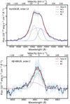 |
Fig. 1 Line proflies of Hα in the redU arm (top panel), and Hβ in the redL arm (bottom panel) of the UVES spectrum of 2M1115. We note that NC and BC indicate the narrow component and broad component of the total Gaussian fit to the profile, respectively. The flux uncertainties are shown as vertical error bars and represent the weighted standard deviation among the four observations. The velocity was set with respect to the rest-frame wavelength (in air) of the respective lines. |
4.2 Asymmetry in the line profiles
Among the detected H I lines, Hα and Hβ show clear asymmetries in their line profiles. Following Ringqvist et al. (2023), we fitted multi-component Gaussian models to their line profiles, composed of a combination of narrow and broad components (NCs and BCs, respectively). The best model for each line was determined as the one that gave the least χ2, calculated as
![Mathematical equation: ${\chi ^2} = \sum\limits_i {{{\left[ {{{{N_i} - fi} \over {{\sigma _i}}}} \right]}^2}} ,$](/articles/aa/full_html/2024/11/aa50881-24/aa50881-24-eq6.png) (1)
(1)
where σi is the error in the measurement Ni and fi is the corresponding model prediction. The resulting line profile fits for Hα and Hβ are given in Figure 1 and their characteristics are given in Table D.1. Such a multi-component profile fit is reasonable, as explained in the 1D planet-surface shock model of accretion in Aoyama et al. (2018, 2020, 2021), where the hotter (≳105 K) gas in the immediate post-shock region is receding away from the observer into the planet and this leads to a broad, redshifted profile. Comparatively, gas coming from deeper below the shock region originates at lower temperatures (≈104 K) and is thus narrower. In Section 5, we discuss the significance of these profile fits further.
We also fitted the obtained H I line profiles with predictions from Aoyama et al. (2020, 2021) models as a function of pre-shock velocity v0 and pre-shock number density n0. We allowed the model grid to vary from v0 = 50–200 km s−1 and n0 = 109−1014 cm−3 during the fitting process. The observed Hα emission from the target is quite strong compared to the other H I lines. One reason could be the strong dependence of extinction on wavelength, as seen in PDS 70b and c (Hashimoto et al. 2020). Upon setting the extinction to a high value of Av = 3.5 mag, the model shows a good fit to both Hα and Hβ, but very weak predictions for H6 and H7, making the overall model prediction unsatisfactory. A simple interpretation of this analysis could be that the main origin for Hα emission is not the shock-heated region. Aoyama et al. (in prep.) have demonstrated similar, strong contamination for Hα with other than shock-heated gas (e.g. gas along accretion columns or chromospheric activity) using archival data for massive planets >10 MJup. In these cases the line profiles show better agreement with the model for Hβ and higher order lines, upon excluding Hα from the analysis. Accordingly, we repeated our fitting process by including only the lines H4–H7 and fixing the extinction to Av = 0 mag. The resulting fit reproduces the H4–H7 line profiles very well within their flux uncertainties, with model parameters of  km s−1 and log(n0/cm−3) =
  (see Appendix E for details on the fitting process and the inference of uncertainties on these parameters). This strongly suggests that shock emission contributes only minimally to Hα. On the other hand, the higher-order Balmer lines H4–H7 are well reproduced with the shock emission model in this analysis. As seen from the observed hydrogen line spectral profiles in T-Tauri stars, higherorder Balmer lines are generally less contaminated by emission from accretion columns since the lower temperature of the accretion flow at these low-mass stars allows only the lower-order hydrogen lines, such as Ha, to be bright (see Hartmann et al. 2016). A similar trend can be expected in planetary-mass objects as well. As a result, there is less likelihood for the detected H4–H7 lines to have a contribution from the accretion columns. In Section 5, we show that the expected level of chromospheric emission based on the target’s temperature is not significant compared to the observed Balmer emission. However, since chromospheric activity can also be non-thermal, contamination from this source cannot be completely ruled out with the current data.
Considering the pre-shock gas velocity from the best-fit Aoyama et al. (2020, 2021) model as the free-fall velocity of the in-falling gas, we can derive a mass estimate Mp for the accreting PMC (Aoyama & Ikoma 2019) using
 (2)
(2)
The existing radius estimate for 2M1115 in the literature (Rp = 1.3 ± 0.2 RJup; Theissen et al. 2018) is based on an earlier photometric distance measurement of 37 ± 6 pc from before the Gaia DR3 observation of the target. With the more accurate Gaia-parallax-based distance measurement for the target (45.21 ± 2.20 pc), the radius estimate was in need of revision. For this purpose, we performed an SED fit to the existing photometry of 2M1115 using BT-Settl AGSS 20009 (Allard et al. 2012, 2013; Asplund et al. 2009), AMES-Dusty (Chabrier et al. 2000; Allard et al. 2001), and DRIFT-PHOENIX (Baron et al. 2003; Helling et al. 2008; Witte et al. 2011) model photospheres via the Virtual Observatory SED analyzer (VOSA4; Bayo et al. 2008) version 7.5 (see Appendix H for details). The corresponding parameters for the target from the best-fitting models are Teff = 1816 ± 63 K, log(Lbol/L⊙) = −3.63 ± 0.05, and Rp = 1.5 ± 0.1 RJup. With this radius estimate and  km s−1, we get a mass estimate of
  MJup for 2M1115. The resulting 1σ mass range (2–14 MJup) implies a lower mass for the object than in the literature (see Table 1).
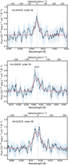 |
Fig. 2 Line profiles of (upper panel) Hγ in order 34, (middle panel) Hγ in order 35, and (lower panel) Hδ in order 28 detected in the UVES spectrum for 2M1115 in the blue arm. The flux uncertainties are shown as vertical error bars and represent the weighted standard deviation among the four observations. The velocity was set with respect to the rest-frame wavelength (in air) of the respective lines. |
Integrated fluxes, luminosities, and mass accretion rates for the H I lines detected in the 2M1115 UVES spectrum.
4.3 Mass accretion rate for 2M1115
The H I line luminosities (Lline) can be used to estimate accretion luminosities (Lacc) for 2M1115 using scaling relations of the form
 (3)
(3)
where a and b represent the fit coefficients for the scaling relations of each transition. Given the existing estimate of the mass range for the target (Mp ≈ 7–21 MJup), we used Lline−Lacc relations from Aoyama et al. (2021) for the lines H3–H7, formulated for planetary-mass objects (Mp ≈ 2–20 MJup) based on spectrally resolved, non-equilibrium models for hydrogen emission due to a shock on the planetary surface. The resulting accretion luminosities for the target are listed in Table 2.
We derived mass accretion rates (Ṁacc) for 2M1115 from the estimated accretion luminosities of the H I lines based on the established relation for stars
 (4)
(4)
where G is the gravitational constant, Mp represents the mass of the accreting object, Rp its radius, and Rin the inner radius of a truncated circumplanetary disk in a magnetospheric accre-tion scenario (Hartmann et al. 2016). Upon setting Rin = 5 Rp (Gullbring et al. 1998; Alcalá et al. 2017; Ringqvist et al. 2023), Ṁacc ≈ LaccRp/GMp, which remains valid for a planet-surface shock scenario under the assumption that the entire kinetic energy from the shock is converted into radiation (Marleau et al. 2019).
With Rp =1.5 ± 0.1 RJup (this work) and Mp =14 ± 7 MJup (Theissen et al. 2018), we derived a mass accretion rate for 2M1115 from each detected H I line (H3–H7) using Eq. (4) (listed in Table 2). The average mass accretion rate obtained thusly is log(Ṁacc/MJup yr−1) = −7.86 ± 0.48 for the target. In Section 4.2, we provide evidence for Hα possessing a significant contribution from non-shock emission, with the likely sources being accretion columns or chromospheric activity. Although the expected emission from the latter at the temperature of 2M1115 is lower by several orders of magnitude than the level of emission seen in these observations (see Section 5), any minor contribu-tion from chromospheric activity to the detected Hα emission cannot be completely ruled out. Using Lline–Lacc scaling laws that assume that the entire line luminosity contributes to accretion luminosity should hence be done so with caution in this case. However, since the current observational data on the target limit a quantification of this non-shock contribution, or further analysis of its nature, we have considered the total Hα luminosity from the target while using scaling laws to estimate its accretion lumi-nosity, and subsequently its mass accretion rate, in this work. The Aoyama et al. (2021) scaling laws also come with associated model-dependent uncertainties that would result in systematic uncertainties in the subsequent calculation of Lacc and Ṁacc.
In Appendix I, we estimated H3–H7 line fluxes for 2M1115 from its existing, moderate-resolution SDSS DR9 (Ahn et al. 2012) and DR12 (Alam et al. 2015) spectra and, subsequently, derived mass accretion rates log(Ṁacc/MJup yr−1) of −8.00 ± 0.32 and −7.62 ± 0.32 from DR9 and DR12, respectively. The mass accretion rate estimate from the UVES data are ~0.3σ higher and ~0.5σ lower (in dex) than those from SDSS DR9 and DR12, respectively. We discuss this difference further in Section 5.
Together with the mass accretion rate and the best-fit pre-shock velocity and number density from the analy-sis within the planet-surface shock framework (Section 4.2), we can estimate the fraction of the planetary surface from where the H I line radiation is emitted, the filling factor ff (Aoyama & Ikoma 2019), as
 (5)
(5)
Here, µ′ is the mean weight per hydrogen nucleus. The resulting filling factor obtained from the best-fit n0, v0 values and the aver-age mass accretion rate obtained above from our observations is 0.03%.
We also estimated accretion rates using Lline–Lacc scaling relations from Alcalá et al. (2017), which were derived empir-ically based on a sample of young, low-mass stars. Contrary to Aoyama et al. (2021), these relations assume that H I emission, in the case of stellar accretion, comes from gas in the accretion columns following the magnetic field lines onto the stellar surface. The Lacc and Ṁacc values estimated from the detected H I lines based on these stellar scaling relations are also listed in Table 2. The average mass accretion rate estimated thusly for 2M1115 is log(Ṁacc/MJup yr−1) = −8.75±0.64. This is ~1 dex lower than the estimate from Aoyama et al. (2021) scaling rela-tions, similar to what was seen in Ringqvist et al. (2023) for Delorme 1 (AB)b.
As an independent check, we also derived a mass accretion rate for the target using the 10% width (W10) of its Hα line. Natta et al. (2004) developed an empirical relation between Ṁacc and Hα W10, for accretors with W10 ≳ 200 km s−1 (Jayawardhana et al. 2003), using a sample of very low-mass objects and T-Tauri stars, spanning a mass range of 0.04 ≲ M★/M⊙ ≲ 0.8, given by
 (6)
(6)
where W10 is in km s−1 and Ṁacc is in M⊙ yr−1. Using the measured W10 of the overall Hα profile for the target (199.4 ± 1.2 km s−1), we get an accretion rate of log(Ṁacc/MJup yr−1) = −7.94 ± 0.33, which is consistent with the average Ṁacc estimate from Aoyama et al. (2021) scaling rela-tions within the uncertainties. It is important to note here that values of Ṁacc and Hα 10% width of the sample used in Natta et al. (2004) are mostly not simultaneous measurements, and hence the resulting Ṁacc from the relation should be interpreted with caution. Regardless, the value serves as a cross-check on the mass accretion rate for 2M1115, since it relates the observed Hα width directly to Ṁacc instead of relying on a Lline–Lacc scaling relation.
4.4 Likelihood of being bound to 2M1113
As mentioned in Section 1, the M-type star 2MASS J1113+2110 has been suggested to be likely physically associated with 2M1115, based on their spatial proximity and similarity in age and space motion (Theissen et al. 2018), with a 1.8% probabil-ity of chance alignment between the two. In light of Gaia DR3 observations of these objects, we revisited their properties. Similar to Theissen et al. (2018), neither 2M1115 nor 2M1113 are seen belonging to any of the known stellar associations as implied from the membership probabilities calculated from the Bayesian Analysis for Nearby Young AssociatioNs Σ (BANYAN Σ; Gagné et al. 2018) tool based on their proper motion, parallax, distance, and radial velocity (RV; both show a 99.9% probability of being a field object). With the new Gaia distance measurements, the projected physical separation corresponding to the 1.62° angular separation between the two is 1.28 pc, approximately the same as the distance to Proxima Centauri from the Sun (1.29 pc; Turbet et al. 2016). Although the proper motion of 2M1113 (µα* = −68.932 ± 0.194 mas yr−1, = −21.985 ± 0.190 mas yr−1; Gaia Collaboration 2023) agrees within ≈ 1.6 mas yr−1 of that of 2M1115, their parallax measurements differ by ≈4.4σ (parallax = 17.34 ± 0.25 mas for 2M1115; Theissen et al. 2018), which reduces the likelihood of the two objects being bound.
To investigate further the possibility that 2M1115 and 2M1113 are physically bound, we calculated the tidal radius (Rtid) of 2M1113 as Rtid = 1.35 pc × (M★/M⊙)⅓ (Jiang & Tremaine 2010; Mamajek et al. 2013). Based on the Theissen et al. (2018) mass range for the object (45–75 MJup), we assumed a mass of 60 ± 15 MJup, resulting in Rtid = 0.52 ± 0.04 pc. At the distance of 2M1113 (57.66 ± 0.84 pc), this corresponds to a tidal radius of 0.52 ± 0.04°. 2M1115 being at a projected angular separation of 1.62° is significantly beyond the tidal influence of 2M1113. Hence the hypothesis that the two are gravitationally bound can be ruled out. However, given the similar proper motion and RVs (RV= −10.1 ± 0.3 km s−1 for 2M1113; Theissen et al. 2018), there is a possibility of the two objects sharing the same dynamical origin.
5 Discussion
From our observations using VLT/UVES at a high resolution of R ~ 50 000 across the optical to near-UV wavelength range, we have detected the first resolved H I emission from the young, isolated, L2γ dwarf 2MASS J1115+1937, from Hα to H7. The Hα emission from the object is broad, with its width measured at 10% peak flux, W10 = 199.4 ± 1.2 km s−1. This puts 2M1115 right at the 200 km s−1 threshold for accretion in very low-mass stars and brown dwarfs (Mohanty et al. 2005). Together with the asymmetries in the observed Hα and Hβ profiles and the tentative detection of the He I emission at 6678 Å (refer Table G.1), the object displays clear signs of accretion, corroborated by the indicative presence of a disk around the object as seen from its SED (see Figure H.1).
Mohanty et al. (2005) and Muzerolle et al. (2005) presented extensive catalogues of observed Hα profiles from low-mass stars and sub-stellar objects, along with their mass accretion rates measured from their Ca II (λ8662 Å) flux in the former, or using radiative transfer modelling based on magnetospheric accretion flows (Muzerolle et al. 2001) in the latter. Our profile fit for Hα emission from 2M1115 agrees well with that of the M7-type dwarf CFHT BD Tau 4 from Mohanty et al. (2005), in addition to those of Cha Hα 1 and KPNO 6 of spectral types M7.75 and M8.5 from Muzerolle et al. (2005), respectively (see Figure F.1). CFHT BD Tau 4, of mass ~60 MJup, is classified as a possible accretor based on its Hα 10% width, the presence of a disk, and Ca II (λ8662 Å) emission, with a reported mass accretion rate Ṁacc ≈ 1.3 × 10⁻⁸ MJup yr−1 estimated from the latter (Mohanty et al. 2005). The model-predicted profile fits in Muzerolle et al. (2005) to the accretors Cha Hα 1 (~35 MJup) and KPNO 6 (~25 MJup) indicate mass accretion rates of 5.25 × 10⁻⁹ and 4.17 × 10⁻⁹ MJup yr–1, respectively. The average mass accretion rate obtained for 2M1115 using Aoyama et al. (2021) scaling relations  agree within ~1.1σ with the estimated Ṁacc for all three objects, showing consistency with the matching line profiles. The Ṁacc obtained based on the Hα W10 (Natta et al. 2004),
  , also agrees well with those of these three accretors. On the other hand, the average Ṁacc obtained from the (Alcalá et al. 2017) scaling relations
  is an order of magnitude lower than that of CFHT BD Tau 4, but it agrees with those of Cha Hα 1 and KPNO 6.
The associated accretion luminosity derived for 2M1115 from Aoyama et al. (2021) scaling relations is, on average, log(Lacc/L⊙) = –4.54 ± 0.38. The Teff-dependent chromospheric noise limit from Manara et al. (2013) (see also Venuti et al. 2019) derived from a sample of non-accreting young stellar objects with Teff ≤ 4000 K is given by
 (7)
(7)
This limit describes the simulated luminosity from a non-accreting young star of a certain spectral type (or Teff) solely due to its chromospheric activity. The Teff = 1816 ± 63 K we derived translates into a chromospheric noise limit of log(Lacc,noise/Lbol) = −4.29 ± 2.50 for 2M1115. Together with the estimated Lbol from its SED fit, this corresponds to a luminosity limit of log(Lacc,noise/L⊙) = −7.92 ± 2.50. The estimated accre-tion luminosity from its H I emission is higher by more than three orders of magnitude (3.4 dex) compared to this noise limit. Although the relation is derived from K- and M-type stars and may have uncertainties when extrapolated to planetary tempera-tures, it is unlikely that the true Lacc,noise at these temperatures is higher by several orders of magnitude than what is derived from the extrapolation, to reach the Lacc level estimated for 2M1115 from these observations. Thus, there is very little likelihood that all the H I lines from 2M1115 are solely due to its chromospheric activity.
Among the detected H I lines, H6 and H7 show similar velocity shifts (within uncertainties) as the systemic RV of −14 ± 7 km s−1 (refer Table D.1), along with H5 in order 35 and Hβ in order 3. H5 in order 34 is slightly blue-shifted relative to the systemic velocity. The Hβ profile in order 2 has both broad and narrow components, which are blue-shifted (~−14 km s−1) and red-shifted (~+8 km s−1) relative to the systemic RV. The Hα profile has two NCs in addition to the BC. The BC is red-shifted relative to the system velocity, as predicted by the Aoyama et al. (2018, 2021) models (discussed in Section 4.2), along with a blue-shifted NC; however, the red-shifted NC cannot be explained within the planetary accretion shock framework. The Hα emission is also significantly stronger than other detected H I lines, and does not agree with a predicted flux from the planet-surface shock model that fits the rest of the H I lines very well. This could, as discussed in Section 4.2, point to a partial or even dominating contribution from mechanisms other than shock-heating for Hα emission such as heating along the accretion columns or chromospheric activity. The best-fit planet-surface shock model that fits all detected H I lines other than Hα predicts a filling factor of 0.03%, which hints at a magneto-spheric accretion geometry for 2M1115 (Ringqvist et al. 2023). This provides tentative, indirect evidence for a magnetic field on such a low-mass and young isolated object.
Moderate-resolution SDSS spectra available for the target from DR9 (March 2007) and DR12 (April 2012) epochs, together with the UVES epoch (June 2023) data, facilitate an analysis of the accretion over time. From Tables 2 and H.1, it can be inferred that the Hα flux decreases by ~7% between 2007 and 2012, and then increases by ~20% between 2012 and 2023. On the other hand, line fluxes for Hβ–H7 increase by 200–300% between 2007 and 2012, and decrease by ~50–80% between 2012 and 2023 for Hβ, H5, and H7, and by ~15% for H6. On average, the H I accretion luminosity in the DR12 epoch (log(Lacc/L⊙) = −4.30 ± 0.14) is higher by ~150% from the DR9 epoch (log(Lacc/L⊙) = −4.68 ± 0.14) and by ~75% from the UVES epoch (log(Lacc/L⊙) = −4.54 ± 0.38). The average mass accretion rates estimated from all the H I lines in all three epochs imply the same progression, varying as Ṁacc ≈ 1 × 10⁻⁸, 2.4 × 10⁻⁸, and 1.4 × 10⁻⁸ MJup yr−1 between the DR9, DR12, and UVES epochs, respectively. The trend seen from the hydro-gen emission over the three epochs suggests a variability in accretion in the target, and could benefit from a future detailed time-resolved monitoring of the emission lines.
A major source of uncertainty in the analysis presented in this work is the loosely constrained mass of the target. The previously reported mass for the target in the literature (7– 21 MJup; Theissen et al. 2018) was estimated from evolutionary models using the temperature estimate from the SED fit to its zJHKS W1 photometry based on the photometric distance esti-mate of 37 pc, and the age range 5–45 Myr. The lower age limit was roughly based on the end of the accretion phase for brown dwarfs (Mohanty et al. 2005) and the upper age limit was taken as that of the oldest accreting object known to harbour primordial circumstellar material (Boucher et al. 2016). With the revised distance and resulting SED fit discussed in Section 4.3, we attempted to constrain the mass further. Using the updated abso-lute magnitudes in the J, H, and KS bands, from the DUSTY00 atmosphere isochronal models for very low-mass stars and brown dwarfs (Chabrier et al. 2000), we inferred a mass of ~7.5 MJup at 5 Myr and ~21 MJup at 50 Myr. Alternatively, we also interpolated the AMES-Cond (Allard et al. 2001) and BT-Settl (Allard et al. 2012, 2013) model isochronal grids for the temperature from our SED fit (1816 K) in the age range 5–50 Myr. This gives a slightly lower and stricter mass range of 9–15 MJup. The surface gravity (log(g) = 3.83 ± 0.24) and radius from the best-fit atmospheric models to the SED (refer to Appendix H) imply an even lower mass range of 6 ± 4 MJup, while the best-fit Aoyama et al. (2018, 2021) model to the observed H I predicts a mass  (refer Section 4.3). The latter estimate is not quite independent from the former since it was calculated partly based on the radius estimate from the SED fit. Nevertheless, the implied mass range from our analysis is slightly lower than the existing mass range in the literature, but still remains fairly large. Depending on the lowest (2 MJup) to highest (21 MJup) value in the mass range listed for the target here, the esti-mated mass accretion rate (Ṁacc/MJup yr−1) changes by a factor of approximately 1 dex.
Our observations of 2M1115 and the resulting findings demonstrate the great potential of VLT/UVES for studying young, accreting planets. We find that 2M1115 could greatly benefit from further study; better constraints on its age could be placed by obtaining photometry covering a longer wavelength range in its SED. A dynamic, model-independent estimate of its mass can be obtained by studying the disk kinematics using ALMA (ALMA Partnership 2015). Imaging using instruments such as the Mid-Infrared Instrument (MIRI; Wright et al. 2015) aboard the James Webb Space Telescope (JWST) to study the spectral distribution of 2M1115 at MIR wavelengths could also help to constrain the properties of the disk. Further, spectro-scopic observations of 2M1115 in the NIR to study accretion signatures such as Paschen and Brackett emission lines can serve as an independent check on the mass accretion rate and give further insights into the accretion geometry. Monitoring emis-sion lines from the target over various timescales with UVES or other upcoming high-resolution spectrographs such as the Arma-zoNes high Dispersion Echelle Spectrograph (ANDES, formerly known as HIRES; Marconi et al. 2021) can help investigate accretion variability. Finally, continued monitoring of 2M1115’s space motion could help solve the mystery of whether it belongs to undiscovered stellar associations as of yet or whether it has been ejected from currently known ones.
Data availability
The underlying data for the analysis presented in this work are the stacked, flux-calibrated 1D UVES spectrum obtained from the ESO observations on 2023 June 10 and 11, under programme 0111.C-0166(A). The raw science data and calibration prod-ucts are available through ESO Archive Services. The stacked spectrum used in this work and the reduced 2D spectra from both nights of observations are available as ESO Phase 3 sci-ence data products, and are also accessible from Zenodo at DOI 10.5281/zenodo.13884607.
Acknowledgements
M.J. gratefully acknowledges funding from the Knut and Alice Wallenberg Foundation and the Swedish Research Council. G.-D.M. acknowledges the support of the DFG priority program SPP 1992 “Exploring the Diversity of Extrasolar Planets” (MA 9185/1) and from the Swiss National Science Foundation under grant 200021_204847 “PlanetsInTime”. Parts of this work have been carried out within the framework of the NCCR PlanetS sup-ported by the Swiss National Science Foundation. This publication makes use of VOSA, developed under the Spanish Virtual Observatory (https://svo.cab.inta-csic.es) project funded by MCIN/AEI/10.13039/501100011033/ through grant PID2020-112949GB-I00. VOSA has been partially updated by using funding from the European Union’s Horizon 2020 Research and Innovation Programme, under Grant Agreement no. 776403 (EXOPLANETS-A). Funding for SDSS-III has been provided by the Alfred P. Sloan Foundation, the Partici-pating Institutions, the National Science Foundation, and the U.S. Department of Energy Office of Science. The SDSS-III web site is http://www.sdss3.org. SDSS-III is managed by the Astrophysical Research Consortium for the Par-ticipating Institutions of the SDSS-III Collaboration including the University of Arizona, the Brazilian Participation Group, Brookhaven National Labora-tory, Carnegie Mellon University, University of Florida, the French Participation Group, the German Participation Group, Harvard University, the Instituto de Astrofisica de Canarias, the Michigan State/Notre Dame/JINA Participation Group, Johns Hopkins University, Lawrence Berkeley National Laboratory, Max Planck Institute for Astrophysics, Max Planck Institute for Extraterres-trial Physics, New Mexico State University, New York University, Ohio State University, Pennsylvania State University, University of Portsmouth, Princeton University, the Spanish Participation Group, University of Tokyo, University of Utah, Vanderbilt University, University of Virginia, University of Washington, and Yale University.
Appendix A Details of observations
Table A.1 gives the observing log for 2M1115 with VLT/UVES during 2023 June 10–11, as part of the ESO programme 0111.C-0166(A). The integration time was 740 s for each observation with the number of integrations, NDIT=1. The seeing measure-ments quoted here are estimated from the FWHM (full width at half maximum) of the 2D spatial PSF of Hα line from the data.
Observing log for the VLT/UVES observations of 2M1115 on 2023 June 10, 11.
Appendix B Flux calibration
The moderate-resolution spectrum from SDSS DR12 (Alam et al. 2015) and DR9 (Ahn et al. 2012) does not reveal any sig-nificant continuum for 2M1115 in the relevant wavelength range for the UVES data. The stacked UVES spectrum when binned to ~5 Å resolution also does not show any continuum, except for a faint continuum that begins to appear near the higher wavelength end of the upper red arm (> 6000 Å). With no considerable continuum emission from the object, flux calibration based on a theoretical model fit to the object’s SED would not be ideal since the photometric bands in the optical wavelength range will be mostly dominated by the flux from the emission lines.
An alternative method would be to calibrate the object’s flux based on the observing instrument’s response curve. For this purpose, we use the observations of the standard star LTT 6248 taken with UVES on 2023 June 11 with the same observ-ing setup as 2M1115. A well-calibrated spectrum for this star exists in the literature (Rubin et al. 2022) in the required wave-length range. The UVES spectrum for LTT 6248 was extracted using the default ESO pipeline and was corrected for atmo-spheric transmission at an air mass of 1.7 corresponding to its observing conditions, using the sky transmission curve obtained from ESO’s SKYCALC Sky Model Calculator5. The instrument response for UVES was derived by dividing the spectropho-tometric calibrated spectrum of LTT 6248 from Rubin et al. (2022) with its uncalibrated UVES spectrum normalised for the corresponding integration time (500 s).
We then flux calibrated the 2M1115 UVES spectrum by first correcting it for atmospheric transmission at the average air mass of its observations (1.415), then normalising it for its integration time of 740 s and finally multiplying it by the instrument response curve derived above. The resulting calibrated spectrum for the target shows consistency between the integrated flux for H I emission lines with those from earlier SDSS epochs (refer Table I.1).
Appendix C Identification of potential lines
Potential emission lines were selected from the stacked spec-trum and classified as confirmed or tentative detection based on a detection confidence determined as described here. For each potential line identified in the spectrum, a region of 20 Å width is defined around the line, usually centred on the line except when the line is near the beginning or end of an order (in which case the region is shifted by 5 Å away from the noisier part). The local noise is calculated as the standard deviation within this region, avoiding ±2 Å around the centre of the line. A single Gaussian is then fit to the line and the detection confidence is determined as the strength of the line, estimated as the peak of the resulting Gaussian fit. Identified emission lines are classified as confirmed detections if the corresponding detection confidence is higher than 5σ, with σ being the local noise. We note that a high threshold of 5σ is used since we do fit for a continuum in the spectrum (as discussed in Appendix B) and thus may be under-estimating the corresponding noise. Alternatively, if the line is recurrent in two subsequent orders, and the rms of the two line strengths is higher than 5σ, it is also classified as a confirmed detection. Lines identified similarly with a confidence of 3–5σ are classified as tentative detections.
Appendix D Characteristics of H I line profiles
Figure D.1 illustrate the Gaussian fits to the profile of the tentatively detected Hβ in order 3 of the redL arm (4.3σ) and H7 in order 25 of the blue arm (3.6σ). H7 shows a slight increase in flux at the blue side of the line, indicative of a possible blend-ing with either Fe I at 3970.63 Å or Cr I at 3969.74 Å. H7 was also detected in order 24, but since the detection confidence is only 1.7σ, we do not include it in our analysis. We also detected a clear flux increase in orders 20 and 21 of the blue arm corre-sponding to the H9 line at 3835.40 Å (see Figure D.2) but the detection strength for both were not formally significant (1.9σ and 1.7σ respectively) and has not been listed among detections in this work. The characteristics of the line profiles for all the H I emission lines detected in the spectrum are given in Table D.1. Hα and Hβ are best explained with a triple (t) and double (d) Gaussian fits respectively while the rest of the H I lines, being of lower S/N, are fitted with single (s) Gaussians.
 |
Fig. D.1 (Left) Hß detected at 4.3σ- in order 3 of the redL arm, and (Right) H7 line detected at 3.6σ in order 25 of the blue arm of UVES in the 2M1115 data. The red curve indicates the Gaussian fit to the observed flux (blue curve). The blue vertical lines indicate the uncertainty in the flux. The tentatively detected Ca II H (3968.47 Å) at 3.1σ and Fe I (3967.42 Å) at 3.2σ next to H7 are also indicated in the figure. |
 |
Fig. D.2 The flux increase detected at the location of H9 in (Left) order 21, and (Right) order 20 of the blue arm of UVES in the 2M1115 data, at 1.7σ and 1.9σ respectively. Colours and symbols hold the same meaning as in the previous figure. |
Characteristics of the line profiles for H I emission lines detected in the 2M1115 UVES spectrum.
Appendix E Analysis with planet-surface shock model
We fit the observed H3–H7 line profiles of 2M1115 with the Aoyama et al. (2020, 2021) model grids assuming H I line emission from shock at the planet surface.
The quality of the fit was determined by reduced  with χ2 defined as
 (E.1)
(E.1)
Here, σ is the uncertainty in the observed flux Fobs,i for bin i and Fmodel,i is the corresponding flux prediction from the model. The value of ; for the fit is then obtained by dividing χ2 by the degree of freedom, which is the number of bins used in the fitting process. A
  (light blue) indicates good agreement between the model prediction and the observed profile, and
  (darker blue) indicates that the difference is less than the uncertainty in the flux.
Hα is significantly brighter than the rest of the H I lines detected; trying to fit for Hα using a high extinction of 3.5 mag shows very poor agreement with H5, H6 and H7 profiles. Hence, Hα has been excluded from the following analysis. For fitting H5, we took the average of its line profiles from orders 34 and 35. For H5-H7, we also masked the bins corresponding to possible contamination from metal lines, as described in Section 4.1 and Appendix D. The resulting quality of the fit improved greatly, with good agreement over a wider parameter range (see Figure E.1) as compared to when these possible metal lines were included in the fitting process. This highlights the importance of the high spectral resolution such as with UVES, which helps identify overlapping metal lines in the line profile.
Among the models that show good agreement with  , adopting a pre-shock gas velocity of v0 = 120 km s−1 and a pre-shock gas density of no = 1014 cm−3 reproduces all the line profiles (H4–H7) very well (see Figure E.2), while others reproduce some of the lines well but not others. The blue region in the figure indicate those values of v0, n0 for which fitting residuals are not statistically significant at the 1σ level. The pre-shock gas parameters over this region range from v0 = 80 – 200 km s−1 and n0 = 109 − 1014 cm−3. Accordingly, we define the uncertainties in the best-fit model parameters as
  and
and  . The upper uncertainty in n0 is set as 0 since the best-fit value reaches the edge of the model grid.
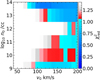 |
Fig. E.1 Results from fitting Aoyama et al. (2020, 2021) model-grid to the observed H4-H7 line profiles of 2M1115. The model-grid allows n0 to range from 109 − 1014 cm−3 and v0 to range from 50 − 200 km s−1. The corresponding |


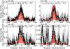 |
Fig. E.2 The SED with Aoyama et al. (2020, 2021) model corresponding to |

Appendix F Comparison of H3 with standard line profiles in the literature
The comparison of the obtained Hα line profile for the target with the best-matching Hα profiles from Muzerolle et al. (2005) and Mohanty et al. (2005) is illustrated in Figure F.1. The line profile for all the objects have been normalised by their peak flux for the sake of comparison. The Hα profile for 2M1115 in this plot has been corrected for the line’s observed radial velocity shift (−7.3 + 1.4 km s−1) as determined from a single Gaussian fit to its line profile.
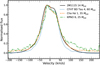 |
Fig. F.1 Profile fit to Hα emission from 2M1115 compared to normalised Hα profiles for CFHT BD Tau 4 from Mohanty et al. (2005) and Cha Hα 1, KPNO 6 from Muzerolle et al. (2005). The Hα profile for 2M1115 in this plot has been corrected for its observed velocity shift. |
Appendix G Non-Hydrogen line detections
Apart from H I lines, we also detected He I emission (see Figure G.1) and several metal lines including Ca II H, Fe I, Cr I and Ti I. He I emission at 5876 Å was detected at high confidence (8.6σ) while He I emission at 6678 Å was detected tentatively (3.2σ). Ca II H was detected tentatively in order 25 of the blue arm (see Figure D.1, right panel) at 3.4σ; the line also recurred in order 24 but at only 1.6σ with no formal significance to include in the detection list. Both the Ca II H detections were at an RV of ~25 km s−1, much redder compared to the systemic RV of −14 ± 7 km s−1. Among the possible metal lines detected (all < 5σ), Fe I emission lines at λ3967.42, 4970.50, 4986.22, and 5684.43 Å were detected at similarly redder RV shifts (~17-35 km s−1), while Fe I emission lines at 4839.54 and 6703.57 Å were detected at bluer RV shifts (~− 25 km s−1) compared to the systemic velocity. We note that this is different from the expected behaviour of metal lines as seen from the stellar cases, which adhere more or less to the systemic velocity (Sicilia-Aguilar et al. 2015). Table G.1 lists the characteristics of the line profiles for all the non-hydrogen lines detected in the data.
 |
Fig. G.1 Line profiles of He I at (Left) 5876 Å and (Right) 6678 Å detected in the orders 1 and 14 of the UVES redU arm at 8.6σ and 3.2σ respectively in the 2M1115 data. Colours and symbols hold the same meaning as in previous figures. |
Characteristics of the line profiles for confirmed and tentative non-Hydrogen lines detected in the 2M1115 UVES spectrum.
Appendix H Fitting atmospheric models to 2M1115 SED
Using VOSA, we queried the existing SDSS (u, g, r, i, z), Gaia DR3 (G, Gbp, Grp), 2MASS (J, H, KS) and WISE (W1, W2, W3, W4) photometry of 2M1115. Since W4 magnitude is a lower limit, we exclude it from the analysis and fit the remaining 14 photometry points (refer Table H.1) with BT-Settl AGSS2009 (Allard et al. 2012, 2013), AMES-Dusty (Chabrier et al. 2000; Allard et al. 2001) and DRIFT-PHOENIX (Baron et al. 2003; Helling et al. 2008; Witte et al. 2011) atmospheric models constrained to near-solar metallicities (−0.5 to 0.5), log(g) range 3—4 (based on the spectral type L2γ; Kirkpatrick 2005; Theissen et al. 2018) and a temperature range of 1200-2500 K (based on existing Teff estimate of  ; Theissen et al. 2018). The extinction is currently unknown for the object; but it is still well within the Local Bubble given its location and hence extinction is likely negligible. So we assumed AV = 0 for our analysis. We do note, however, that the presence of an accretion disk around the target can lead to some intrinsic extinction within the sys-tem; this extinction is currently not constrained due to lack of sufficient data, and has not been accounted for in our analysis. Figure H.1 shows the best-fitting model from each of the three model grids that gives the minimum χ2 with the observed photometry. From the Figure, we see a clear near-UV and optical flux excess compared to the model as well as MIR excess prominent towards the W3 band (indicative of a disk around the object), as previously noted in Theissen et al. (2018). The overall best-fit with least χ2 that fits 13 out of the 14 data points (with MIR excess from W3) corresponds to DRIFT-PHOENIX models at Teff = 1800 ± 50 K, log(g) = 4 ± 0.25 and metallicity of 0.3 ± 0.15. VOSA also predicts the object parameters corresponding the least χ2 based on a polynomial fit to the χ2 vs. parameter-value space for each of the model grids used. Additionally, for each model grid, statistical analysis of the top least χ2 fits also gives average values of the best-fitting model parameters. To arrive at the optimal value of the target parameters, we took the set of parameters corresponding to the least χ2 fits, those predicted from the above-mentioned polynomial fit (as long as the value corresponding to the minimum χ2 falls within the constrained parameter range for the fit) as well as those derived from the average of the best-fits, for each of the three model grids. The rms of these sets of values give the following parameters for the target, which we adopt for our analysis: Teff = 1816 ± 63 K, log(g) = 3.83 ± 0.24, metallicity = 0.24 ± 0.13 and the integrated flux Ftot = (3.68 ± 0.28) × 10−12 erg s−1 cm−2. We derived a bolometric luminosity of Lbol = (2.34 ± 0.29) × 10−4 L⊙ based on the obtained Ftot and the Gaia distance for the target. This Lbol together with the obtained Teff above gives a radius of Rp = 1.54 ± 0.14 RJup. As a cross-check on the VOSA results, we also fit the model grids to the SED of 2M1115 by including its SDSS DR12 spectrum (green curve in Figure H.1) instead of the SDSS photometry. The resulting χ2 gives best-fitting models consistent with those from VOSA, adding robustness to the results derived above.
Photometry for 2M1115 used for the SED fit.
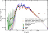 |
Fig. H.1 Least-χ2 fits to the SED of 2M1115 with DRIFT-PHOENIX, BT-Settl-AGSS2009 and AMES-Dusty atmospheric models. The overall best fit with the minimum χ2 corresponds to DRIFT-PHOENIX model at Teff = 1800 ± 50 K, log(g)= 4.0 ± 0.25 and metallicity= 0.3 ± 0.15. The SDSS DR12 spectrum for 2M1115 is also shown, along with its flux uncertainty (grey shaded region). Note that the flux in the WISE W4 band is a 2σ upper limit, denoted by the red downward-pointing arrow, and is not included in the fitting process. The unWISE catalogue (Lang et al. 2016; see https://unwise.me/photsearch/) however reports a W4 detection consistent with this upper limit. |
Appendix I Mass accretion rates from SDSS epochs
We downloaded the existing, public, moderate-resolution optical spectrum for 2M1115 from the two SDSS epochs DR9 (Ahn et al. 2012) and DR12 (Alam et al. 2015) using the SDSS Science Archive Server (SAS). For the detected H I emission lines H3–H7 in the spectrum, we estimated a local continuum as the median flux within +40 A around the line, devoid of ±10 Å region centred on the line. After subtracting the continuum from the spectrum, we fit a single Gaussian profile to the line and estimated the line flux and line luminosities. The uncertainty in the line fluxes are estimated as the rms of the corresponding local continuum. We then used the planetary scaling relations from Aoyama et al. (2021) to estimate accretion luminosities and mass accretion rates for the object, assuming the same values for Mp and Rp as in Section 4.3. The resulting line parameters for the lines H3–H7 are given in Table I.1. The average accretion luminosity log(Lacc/L⊙) calculated from lines H3-H7 is −4.68 ± 0.14 for the DR9 epoch and −4.30 ± 0.14 for the DR12 epoch. The corresponding mass accretion rates log(Ṁacc/MJup yr−1) in the two epochs are −8.00 ± 0.32 and −7.62 ± 0.32 respectively. In the DR9 epoch, the mass accretion rate estimated from Hα seems to be slightly higher than those estimated from H4 and H5 but is consistent with those from H6 and H7 within uncertainties. In the DR12 epoch, the individual mass accretion rates derived from all the H I lines are consistent with each other within the uncertainties, except for that from H7 which is slightly higher.
Line fluxes, luminosities and mass accretion rates for 2M1115 from SDSS DR9 and DR12.
References
- Adams, F. C., Lada, C. J., & Shu, F. H. 1987, ApJ, 312, 788 [NASA ADS] [CrossRef] [Google Scholar]
- Ahn, C. P., Alexandroff, R., Allende Prieto, C., et al. 2012, ApJS, 203, 21 [Google Scholar]
- Alam, S., Albareti, F. D., Allende Prieto, C., et al. 2015, ApJS, 219, 12 [Google Scholar]
- Alcalá, J. M., Manara, C. F., Natta, A., et al. 2017, A&A, 600, A20 [NASA ADS] [CrossRef] [EDP Sciences] [Google Scholar]
- Allard, F., Hauschildt, P. H., Alexander, D. R., Tamanai, A., & Schweitzer, A. 2001, ApJ, 556, 357 [Google Scholar]
- Allard, F., Homeier, D., & Freytag, B. 2012, Philos. Trans. Roy. Soc. Lond. Ser. A, 370, 2765 [NASA ADS] [Google Scholar]
- Allard, F., Homeier, D., & Freytag, B. 2013, Mem. Soc. Astron. Italiana, 84, 1053 [NASA ADS] [Google Scholar]
- ALMA Partnership (Brogan, C. L., et al.) 2015, ApJ, 808, L3 [Google Scholar]
- Aoyama, Y., & Ikoma, M. 2019, ApJ, 885, L29 [NASA ADS] [CrossRef] [Google Scholar]
- Aoyama, Y., Ikoma, M., & Tanigawa, T. 2018, ApJ, 866, 84 [NASA ADS] [CrossRef] [Google Scholar]
- Aoyama, Y., Marleau, G.-D., Mordasini, C., & Ikoma, M. 2020, arXiv e-prints [arXiv:2011.06608] [Google Scholar]
- Aoyama, Y., Marleau, G.-D., Ikoma, M., & Mordasini, C. 2021, ApJ, 917, L30 [CrossRef] [Google Scholar]
- Asplund, M., Grevesse, N., Sauval, A. J., & Scott, P. 2009, ARA&A, 47, 481 [NASA ADS] [CrossRef] [Google Scholar]
- Baron, E., Hauschildt, P. H., Allard, F., et al. 2003, in Modelling of Stellar Atmospheres, 210, eds. N. Piskunov, W. W. Weiss, & D. F. Gray, 19 [NASA ADS] [Google Scholar]
- Batygin, K. 2018, AJ, 155, 178 [NASA ADS] [CrossRef] [Google Scholar]
- Bayo, A., Rodrigo, C., Barrado Y Navascués, D., et al. 2008, A&A, 492, 277 [NASA ADS] [CrossRef] [EDP Sciences] [Google Scholar]
- Benisty, M., Bae, J., Facchini, S., et al. 2021, ApJ, 916, L2 [NASA ADS] [CrossRef] [Google Scholar]
- Betti, S. K., Follette, K. B., Ward-Duong, K., et al. 2022, ApJ, 935, L18 [NASA ADS] [CrossRef] [Google Scholar]
- Blakely, D., Francis, L., Johnstone, D., et al. 2022, ApJ, 931, 3 [NASA ADS] [CrossRef] [Google Scholar]
- Boucher, A., Lafrenière, D., Gagné, J., et al. 2016, ApJ, 832, 50 [NASA ADS] [CrossRef] [Google Scholar]
- Calvet, N., & Gullbring, E. 1998, ApJ, 509, 802 [Google Scholar]
- Chabrier, G., Baraffe, I., Allard, F., & Hauschildt, P. 2000, ApJ, 542, L119 [CrossRef] [Google Scholar]
- Currie, T., Marois, C., Cieza, L., et al. 2019, ApJ, 877, L3 [Google Scholar]
- Cutri, R. M., Skrutskie, M. F., van Dyk, S., et al. 2003, VizieR Online Data Catalog: 2MASS All-Sky Catalog of Point Sources (Cutri+ 2003), VizieR On-line Data Catalog: II/246. Originally published in: 2003yCat.2246 0C [Google Scholar]
- Cutri, R. M., Wright, E. L., Conrow, T., et al. 2021, VizieR Online Data Catalog: AllWISE Data Release (Cutri+ 2013), VizieR On-line Data Catalog: II/328. Originally published in: IPAC/Caltech (2013) [Google Scholar]
- Dekker, H., D’Odorico, S., Kaufer, A., Delabre, B., & Kotzlowski, H. 2000, SPIE Conf. Ser., 4008, 534 [Google Scholar]
- Demars, D., Bonnefoy, M., Dougados, C., et al. 2023, A&A, 676, A123 [NASA ADS] [CrossRef] [EDP Sciences] [Google Scholar]
- Eriksson, S. C., Asensio Torres, R., Janson, M., et al. 2020, A&A, 638, L6 [NASA ADS] [CrossRef] [EDP Sciences] [Google Scholar]
- Gagné, J., Mamajek, E. E., Malo, L., et al. 2018, ApJ, 856, 23 [Google Scholar]
- Gaia Collaboration (Vallenari, A., et al.) 2023, A&A, 674, A1 [NASA ADS] [CrossRef] [EDP Sciences] [Google Scholar]
- Gullbring, E., Hartmann, L., Briceño, C., & Calvet, N. 1998, ApJ, 492, 323 [Google Scholar]
- Haffert, S. Y., Bohn, A. J., de Boer, J., et al. 2019, Nat. Astron., 3, 749 [Google Scholar]
- Hartmann, L. 1998, Accretion Processes in Star Formation (Cambridge University Press) [Google Scholar]
- Hartmann, L., Herczeg, G., & Calvet, N. 2016, ARA&A, 54, 135 [Google Scholar]
- Hashimoto, J., Aoyama, Y., Konishi, M., et al. 2020, AJ, 159, 222 [Google Scholar]
- Helling, C., Woitke, P., & Thi, W. F. 2008, A&A, 485, 547 [NASA ADS] [CrossRef] [EDP Sciences] [Google Scholar]
- Isella, A., Benisty, M., Teague, R., et al. 2019, ApJ, 879, L25 [Google Scholar]
- Jayawardhana, R., Mohanty, S., & Basri, G. 2003, ApJ, 592, 282 [NASA ADS] [CrossRef] [Google Scholar]
- Jiang, Y.-F., & Tremaine, S. 2010, MNRAS, 401, 977 [Google Scholar]
- Kao, M. M., Hallinan, G., Pineda, J. S., Stevenson, D., & Burgasser, A. 2018, ApJS, 237, 25 [NASA ADS] [CrossRef] [Google Scholar]
- Kirkpatrick, J. D. 2005, ARA&A, 43, 195 [NASA ADS] [CrossRef] [Google Scholar]
- Koenigl, A. 1991, ApJ, 370, L39 [Google Scholar]
- Kramida, A., Yu. Ralchenko, Reader, J., & NIST ASD Team 2023, NIST Atomic Spectra Database (ver. 5.11), [Online]. Available: https://physics.nist.gov/asd [2024, May 10] (Gaithersburg, MD: National Institute of Standards and Technology) [Google Scholar]
- Lang, D., Hogg, D. W., & Schlegel, D. J. 2016, AJ, 151, 36 [Google Scholar]
- Luhman, K. L., Tremblin, P., Birkmann, S. M., et al. 2023, ApJ, 949, L36 [NASA ADS] [CrossRef] [Google Scholar]
- Lynden-Bell, D., & Pringle, J. E. 1974, MNRAS, 168, 603 [Google Scholar]
- Mamajek, E. E., Bartlett, J. L., Seifahrt, A., et al. 2013, AJ, 146, 154 [Google Scholar]
- Manara, C. F., Testi, L., Rigliaco, E., et al. 2013, A&A, 551, A107 [NASA ADS] [CrossRef] [EDP Sciences] [Google Scholar]
- Marconi, A., Abreu, M., Adibekyan, V., et al. 2021, The Messenger, 182, 27 [NASA ADS] [Google Scholar]
- Marleau, G.-D., Mordasini, C., & Kuiper, R. 2019, ApJ, 881, 144 [Google Scholar]
- Mendigutía, I., Oudmaijer, R. D., Schneider, P. C., et al. 2018, A&A, 618, L9 [CrossRef] [EDP Sciences] [Google Scholar]
- Mohanty, S., Jayawardhana, R., & Basri, G. 2005, ApJ, 626, 498 [NASA ADS] [CrossRef] [Google Scholar]
- Muzerolle, J., Calvet, N., & Hartmann, L. 2001, ApJ, 550, 944 [Google Scholar]
- Muzerolle, J., Hillenbrand, L., Calvet, N., Briceño, C., & Hartmann, L. 2003, ApJ, 592, 266 [NASA ADS] [CrossRef] [Google Scholar]
- Muzerolle, J., Luhman, K. L., Briceño, C., Hartmann, L., & Calvet, N. 2005, ApJ, 625, 906 [NASA ADS] [CrossRef] [Google Scholar]
- Natta, A., Testi, L., Muzerolle, J., et al. 2004, A&A, 424, 603 [NASA ADS] [CrossRef] [EDP Sciences] [Google Scholar]
- Owen, J. E., & Menou, K. 2016, ApJ, 819, L14 [NASA ADS] [CrossRef] [Google Scholar]
- Rayner, J. T., Toomey, D. W., Onaka, P. M., et al. 2003, PASP, 115, 362 [NASA ADS] [CrossRef] [Google Scholar]
- Rebull, L. M., Hillenbrand, L. A., Strom, S. E., et al. 2000, AJ, 119, 3026 [NASA ADS] [CrossRef] [Google Scholar]
- Reiners, A., & Christensen, U. R. 2010, A&A, 522, A13 [NASA ADS] [CrossRef] [EDP Sciences] [Google Scholar]
- Ringqvist, S. C., Viswanath, G., Aoyama, Y., et al. 2023, A&A, 669, L12 [NASA ADS] [CrossRef] [EDP Sciences] [Google Scholar]
- Rubin, D., Aldering, G., Antilogus, P., et al. 2022, ApJS, 263, 1 [NASA ADS] [CrossRef] [Google Scholar]
- Sallum, S., Follette, K. B., Eisner, J. A., et al. 2015, Nature, 527, 342 [Google Scholar]
- Santamaría-Miranda, A., Cáceres, C., Schreiber, M. R., et al. 2018, MNRAS, 475, 2994 [Google Scholar]
- Santamaría-Miranda, A., Cáceres, C., Schreiber, M. R., et al. 2019, MNRAS, 488, 5852 [CrossRef] [Google Scholar]
- Sicilia-Aguilar, A., Fang, M., Roccatagliata, V., et al. 2015, A&A, 580, A82 [NASA ADS] [CrossRef] [EDP Sciences] [Google Scholar]
- Szulágyi, J., & Mordasini, C. 2017, MNRAS, 465, L64 [CrossRef] [Google Scholar]
- Szulágyi, J., & Ercolano, B. 2020, ApJ, 902, 126 [CrossRef] [Google Scholar]
- Szulágyi, J., Morbidelli, A., Crida, A., & Masset, F. 2014, ApJ, 782, 65 [CrossRef] [Google Scholar]
- Thanathibodee, T., Calvet, N., Bae, J., Muzerolle, J., & Hernández, R. F. 2019, ApJ, 885, 94 [NASA ADS] [CrossRef] [Google Scholar]
- Theissen, C. A., West, A. A., Shippee, G., Burgasser, A. J., & Schmidt, S. J. 2017, AJ, 153, 92 [NASA ADS] [CrossRef] [Google Scholar]
- Theissen, C. A., Burgasser, A. J., Bardalez Gagliuffi, D. C., et al. 2018, ApJ, 853, 75 [NASA ADS] [CrossRef] [Google Scholar]
- Turbet, M., Leconte, J., Selsis, F., et al. 2016, A&A, 596, A112 [NASA ADS] [CrossRef] [EDP Sciences] [Google Scholar]
- Venuti, L., Stelzer, B., Alcalá, J. M., et al. 2019, A&A, 632, A46 [NASA ADS] [CrossRef] [EDP Sciences] [Google Scholar]
- Wagner, K., Follete, K. B., Close, L. M., et al. 2018, ApJ, 863, L8 [Google Scholar]
- Whelan, E. T., Huélamo, N., Alcalá, J. M., et al. 2015, A&A, 579, A48 [NASA ADS] [CrossRef] [EDP Sciences] [Google Scholar]
- Witte, S., Helling, C., Barman, T., Heidrich, N., & Hauschildt, P. H. 2011, A&A, 529, A44 [NASA ADS] [CrossRef] [EDP Sciences] [Google Scholar]
- Wright, G. S., Wright, D., Goodson, G. B., et al. 2015, PASP, 127, 595 [NASA ADS] [CrossRef] [Google Scholar]
- York, D. G., Adelman, J., Anderson, John E.J., et al. 2000, AJ, 120, 1579 [NASA ADS] [CrossRef] [Google Scholar]
- Zhou, Y., Bowler, B. P., Wagner, K. R., et al. 2021, AJ, 161, 244 [NASA ADS] [CrossRef] [Google Scholar]
- Zhu, Z. 2015, ApJ, 799, 16 [Google Scholar]
In this work, all wavelengths have been taken from the NIST Atomic Spectra Database, available at https://www.nist.gov/pml/atomic-spectra-database. The wavelengths are in air.
A similar behaviour has also been observed in the ~40 Myr PMC Delorme 1 (AB)b, where H6 was observed to be overluminous (see Ringqvist et al. 2023).
All Tables
Integrated fluxes, luminosities, and mass accretion rates for the H I lines detected in the 2M1115 UVES spectrum.
Characteristics of the line profiles for H I emission lines detected in the 2M1115 UVES spectrum.
Characteristics of the line profiles for confirmed and tentative non-Hydrogen lines detected in the 2M1115 UVES spectrum.
Line fluxes, luminosities and mass accretion rates for 2M1115 from SDSS DR9 and DR12.
All Figures
|
Fig. 1 Line proflies of Hα in the redU arm (top panel), and Hβ in the redL arm (bottom panel) of the UVES spectrum of 2M1115. We note that NC and BC indicate the narrow component and broad component of the total Gaussian fit to the profile, respectively. The flux uncertainties are shown as vertical error bars and represent the weighted standard deviation among the four observations. The velocity was set with respect to the rest-frame wavelength (in air) of the respective lines. |
| In the text | |
|
Fig. 2 Line profiles of (upper panel) Hγ in order 34, (middle panel) Hγ in order 35, and (lower panel) Hδ in order 28 detected in the UVES spectrum for 2M1115 in the blue arm. The flux uncertainties are shown as vertical error bars and represent the weighted standard deviation among the four observations. The velocity was set with respect to the rest-frame wavelength (in air) of the respective lines. |
| In the text | |
|
Fig. D.1 (Left) Hß detected at 4.3σ- in order 3 of the redL arm, and (Right) H7 line detected at 3.6σ in order 25 of the blue arm of UVES in the 2M1115 data. The red curve indicates the Gaussian fit to the observed flux (blue curve). The blue vertical lines indicate the uncertainty in the flux. The tentatively detected Ca II H (3968.47 Å) at 3.1σ and Fe I (3967.42 Å) at 3.2σ next to H7 are also indicated in the figure. |
| In the text | |
|
Fig. D.2 The flux increase detected at the location of H9 in (Left) order 21, and (Right) order 20 of the blue arm of UVES in the 2M1115 data, at 1.7σ and 1.9σ respectively. Colours and symbols hold the same meaning as in the previous figure. |
| In the text | |
|
Fig. E.1 Results from fitting Aoyama et al. (2020, 2021) model-grid to the observed H4-H7 line profiles of 2M1115. The model-grid allows n0 to range from 109 − 1014 cm−3 and v0 to range from 50 − 200 km s−1. The corresponding |
| In the text | |
|
Fig. E.2 The SED with Aoyama et al. (2020, 2021) model corresponding to |
| In the text | |
|
Fig. F.1 Profile fit to Hα emission from 2M1115 compared to normalised Hα profiles for CFHT BD Tau 4 from Mohanty et al. (2005) and Cha Hα 1, KPNO 6 from Muzerolle et al. (2005). The Hα profile for 2M1115 in this plot has been corrected for its observed velocity shift. |
| In the text | |
|
Fig. G.1 Line profiles of He I at (Left) 5876 Å and (Right) 6678 Å detected in the orders 1 and 14 of the UVES redU arm at 8.6σ and 3.2σ respectively in the 2M1115 data. Colours and symbols hold the same meaning as in previous figures. |
| In the text | |
|
Fig. H.1 Least-χ2 fits to the SED of 2M1115 with DRIFT-PHOENIX, BT-Settl-AGSS2009 and AMES-Dusty atmospheric models. The overall best fit with the minimum χ2 corresponds to DRIFT-PHOENIX model at Teff = 1800 ± 50 K, log(g)= 4.0 ± 0.25 and metallicity= 0.3 ± 0.15. The SDSS DR12 spectrum for 2M1115 is also shown, along with its flux uncertainty (grey shaded region). Note that the flux in the WISE W4 band is a 2σ upper limit, denoted by the red downward-pointing arrow, and is not included in the fitting process. The unWISE catalogue (Lang et al. 2016; see https://unwise.me/photsearch/) however reports a W4 detection consistent with this upper limit. |
| In the text | |
Current usage metrics show cumulative count of Article Views (full-text article views including HTML views, PDF and ePub downloads, according to the available data) and Abstracts Views on Vision4Press platform.
Data correspond to usage on the plateform after 2015. The current usage metrics is available 48-96 hours after online publication and is updated daily on week days.
Initial download of the metrics may take a while.