| Issue |
A&A
Volume 691, November 2024
|
|
|---|---|---|
| Article Number | A350 | |
| Number of page(s) | 23 | |
| Section | Galactic structure, stellar clusters and populations | |
| DOI | https://doi.org/10.1051/0004-6361/202450677 | |
| Published online | 26 November 2024 | |
Calibration of the JAGB method for the Magellanic Clouds and Milky Way from Gaia DR3, considering the role of oxygen-rich AGB stars
1
Vrije Universiteit Brussel, Dienst ELEM,
Pleinlaan 2,
1050
Brussels,
Belgium
2
Koninklijke Sterrenwacht van België,
Ringlaan 3,
1180
Brussels,
Belgium
3
INAF – Osservatorio Astronomico di Padova,
Vicolo dell’Osservatorio 5,
35122
Padova,
Italy
4
Dipartimento di Fisica e Astronomia “Galileo Galilei”, Università di Padova,
Vicolo dell’Osservatorio 3,
35122
Padova,
Italy
5
Space Telescope Science Institute,
3700 San Martin Drive,
Baltimore,
MD
21218,
USA
★ Corresponding author; martin.groenewegen@oma.be
Received:
10
May
2024
Accepted:
5
October
2024
The JAGB method is a new way of measuring distances in the Universe with the use of asymptotic giant branch (AGB) that are situated in a selected region in a J versus J − Ks colour–magnitude diagram (CMD), and relying on the fact that the absolute J magnitude is (almost) constant. It is implicitly assumed in the method that the selected stars are carbon-rich AGB stars (carbon stars). However, as the sample selected to determine MJ is purely colour based, there can also be contamination by oxygen-rich AGB stars in principle. As the ratio of carbon-rich to oxygen-rich stars is known to depend on metallicity and initial mass, the star formation history and age–metallicity relation in a galaxy should influence the value of MJ . The aim of this paper is to look at mixed samples of oxygen-rich and carbon-rich stars for the Large Magellanic Cloud (LMC), Small Magellanic Cloud (SMC), and Milky way (MW) using the Gaia catalogue of long-period variables (LPVs) as a basis. The advantage of this catalogue is that it contains a classification of O- and C-stars based on the analysis of Gaia Rp spectra. The LPV catalogue is correlated with data from the Two Micron All Sky Survey (2MASS) and samples in the LMC, SMC, and the MW are retrieved. Following methods proposed in the literature, we report the mean and median magnitudes of the selected sample using different colour and magnitude cuts and the results of fitting Gaussian and Lorentzian profiles to the luminosity function (LF). For the SMC and LMC, we confirm previous results in the literature. The LFs of the SMC and LMC JAGB stars are clearly different, yet it can be argued that the mean magnitude inside a selection box agrees at the 0.021 mag level. The results of our analysis of the MW sample are less straightforward. The contamination by O-rich stars is substantial for a classical lower limit of (J − Ks)0 = 1.3, and becomes less than 10% only for (J − Ks)0 = 1.5. The sample of AGB stars is smaller than for the MCs for two reasons. Nearby AGB stars (with potentially the best determined parallax) tend to be absent as they saturate in the 2MASS catalogue, and the parallax errors of AGB stars tend to be larger compared to non-AGB stars. Several approaches have been taken to improve the situation but finally the JAGB LF for the MW contains about 130 stars, and the fit of Gaussian and Lorentzian profiles is essentially meaningless. The mean and median magnitudes are fainter than for the MC samples by about 0.4 mag which is not predicted by theory. We do not confirm the claim in the literature that the absolute calibration of the JAGB method is independent of metallicity up to solar metallicity. A reliable calibration of the JAGB method at (near) solar metallicity should await further Gaia data releases, or should be carried out in another environment.
Key words: stars: AGB and post-AGB / stars: carbon / stars: distances / stars: luminosity function, mass function / Magellanic Clouds
© The Authors 2024
 Open Access article, published by EDP Sciences, under the terms of the Creative Commons Attribution License (https://creativecommons.org/licenses/by/4.0), which permits unrestricted use, distribution, and reproduction in any medium, provided the original work is properly cited.
This article is published in open access under the Subscribe to Open model. Subscribe to A&A to support open access publication.
1 Introduction
Nikolaev & Weinberg (2000) presented an infrared Ks versus J − Ks colour–magnitude diagram (CMD) of stars in the Large Magellanic Cloud (LMC) based on Two Micron All Sky Survey (2MASS, Skrutskie 1998; Skrutskie et al. 2006) data and reported a region that consists (almost solely) of carbon-rich asymptotic giant branch (AGB) stars, which they denoted the J region. This, and the fact that the infrared J-band is used to obtain the distance (see below), has led to the stars in this region being referred to as JAGB stars. Nevertheless, the name is confusing there is already a separate spectroscopic group known as the J-type carbon stars (that includes R-, N-, and CH-type C stars; Keenan 1993; Bouigue 1954), that are characterised by strong 13C lines. The origin of this class is not well known, but may be related to binary evolution. In the LMC, the region covered by J-type carbon stars overlaps the region of JAGB stars in the (Ks, J − Ks) CMD (Morgan et al. 2003), which may add to the confusion.
JAGB stars are characterised by their high infrared luminosities and red colours and take only certain values of those variables. As can be seen in the original CMD of Nikolaev & Weinberg (2000; their Fig. 3), the J region is easily separated from the other groups by considering a range in colour. Bluewards of J − Ks ∼ 1.3–1.4 mag (regions F and G), the distribution of oxygen-rich AGB stars and red giant branch (RGB) stars stops abruptly at this boundary, illustrating the difference in colour between O-rich and C-rich AGB stars in the general population. Redwards, the limit of the JAGB stars is put at J − Ks = 2.0 mag to minimise the contamination of extreme carbon stars (region K) whose dusty envelopes cause the extreme red colours. The location of the predominantly C stars in this region is understood theoretically (Marigo et al. 2003).
Nikolaev & Weinberg (2000) and Weinberg & Nikolaev (2001) discuss the use of the stars in region J as standard candles; not in terms of their J-band magnitude, but in connection to the fact that many AGB stars are long-period variables (LPVs), and in particular large-amplitude Mira variables. These authors take 79 C- and O-rich LPVs from Glass et al. (1990), and when restricting the analysis to the 14 Miras in the range 1.4 < (J −Ks) < 1.9 mag, they derive the relation Ks = −(0.99 ± 0.80) (J −Ks) + (12.36 ± 1.33). From this, it follows that Ks + 0.99 (J −Ks) ≈ J = 12.36 mag and with the distance modulus (DM) of 18.5 (± 0.1) (used by Nikolaev & Weinberg 2000), one finds that MJ ≈ −6.15 mag. This result was not explicitly discussed in Weinberg & Nikolaev (2001) and went seemingly unnoticed until Madore & Freedman (2020) pointed out this property and introduced the JAGB method for distance determination.
It is of historical interest to point out that Richer et al. (1984) used the mean I-band magnitude of seven carbon stars in NGC 205 to derive the distance to this galaxy. This was possible due to the use of narrow-band filters (centred on a TiO and a CN band, thus distinguishing directly between C and late-type M stars; see Palmer & Wing 1982; Aaronson et al. 1984; Richer et al. 1984; Cook et al. 1986) developed at that time and the V, R, and/or I bands as continuum filters. Two decades later, Battinelli & Demers (2005a,b) presented the final results of their homogeneous survey of carbon stars in nearby galaxies using these filters. They also focussed on the I band (although they did point out the potential of using near-infrared (NIR) photometry), and found a weak dependence of MI on metallicity, with the more metal-poor systems being brighter1.
Madore & Freedman (2020) selected stars in the box 1.30 < (J − K) < 2.00, corrected for extinction, and determined mean magnitudes of −6.22 ± 0.01 ± 0.03 mag for the Large Magellanic Cloud (LMC) and −6.18 ± 0.01 ± 0.05 mag for the Small Magellanic Cloud (SMC; see Sect. 4.3). Freedman & Madore (2020) provide some additional details on the calibration of the LMC, adopt Mj = −6.20 ± 0.037 mag based on the SMC and LMC, and then apply the method to 14 nearby galaxies.
Independently, the J mag luminosity function (LF) of C stars in the SMC, LMC, and Milky Way (MW) was investigated by Ripoche et al. (2020) using very similar techniques and 2MASS data. These authors used a slightly different colour box, namely 1.4 < (J − Ks)0 < 2.0, and determined the absolute magnitude using the median. They also used catalogues of spectroscopically confirmed C stars to provide the absolute magnitude of both the entirety of the stars in the colour box and the confirmed C stars. Ripoche et al. (2020) find MJ values for the SMC and LMC that are significantly different from each other, and are different from the values found by Madore & Freedman (2020) and Freedman & Madore (2020). Their value for the MW (−5.601 ± 0.026 mag) is significantly fainter than that for the MCs. They also fins a significantly wider LF for the MW (0.67 mag) than for the LMC (0.35 mag) and SMC (0.37 mag), which they attribute to differences in metallicity and star formation history.
Parada et al. (2021) follow Ripoche et al. (2020) in using the median magnitude, but additionally also fit a Lorentzian profile to determine the skewness and kurtosis of the LF. Depending on the skewness of the LF in the target galaxy, either the LMC or the SMC is used as the calibrator galaxy. This method is used to derive the distance to IC 1613 and NGC 6822. Parada et al. (2023) expand this work to a larger sample of galaxies and introduced an unbinned maximum likelihood estimator to determine the parameters of the Lorentzian profile. The method is applied to NGC 6822, IC 1613, NGC 3109, and WLM. These authors also estimated the distance to these galaxies using the tip of the red giant branch (TRGB) method, and found good agreement.
Zgirski et al. (2021) fit the LF with a function consisting of a Gaussian plus a second-degree polynomial. The calibration in the LMC and the application to the SMC WLM, NGC 6822, and NGC 3109 used a colour box of 1.30 < (J − K)0 < 2.0 mag, while for M33, NGC 55, NGC 247, NGC 300, and NGC 7793, which show visible contamination on the blue side, the box is 1.45 < (J − K)0 < 2.0. In all cases these authors adopt a selection box with a height of 2.5 mag in J.
Lee et al. (2021) present a calibration of the JAGB method for the MW using Gaia (Gaia Collaboration 2016) data release 3 (GDR3; Gaia Collaboration 2023). These authors used two catalogues of confirmed C stars2 and correlated them with the 2MASS catalogue and obtained Gaia-based distances from Bailer-Jones et al. (2021). A selection on parallax error (stars with σπ/π > 0.2 were eliminated) and on the quality of the astrometric solution (re-normalised unit weight error RUWE < 2.0) was made. In the box 1.40 < (J − Ks) < 2.00, 153 stars remained and based on the median, their final result was MJ = −6.14 ± 0.05 (statistical error) ±0.11 (systematic error) mag. We note that this value is the apparent absolute magnitude, and is not corrected for extinction (see the last sentence in their Sect. 3)3.
Madore et al. (2022) consider the calibration in the MW by using AGB stars in MW open clusters (OCs), as compiled by Marigo et al. (2022). Based on 17 JAGB stars they derive MJ = −6.40 mag with a scatter of 0.40 and an error on the mean of 0.10 mag. Considering the MW calibration by Lee et al. (2021) mentioned above, Madore et al. (2022) obtain a weighted average of MJ = −6.20 ± 0.01 (stat) ±0.04 (sys) mag to claim consistency between the SMC, LMC, and MW with no evidence for a dependence on metallicity. In trying to reproduce Fig. 1 in Madore et al. (2022; see Fig. F.1) it was discovered that these authors must have used a colour selection of 1.20 ≤ (J − Ks)0 < 2.0, which was not explicitly mentioned in their paper, and is different from what was used in Lee et al. (2021). In addition, Table 2 in Marigo et al. (2022) contains the spectral types of a subset of AGB stars in OCs that shows that 4 of the 17 stars are of spectral type M, MS, or S, and only 5 are confirmed C stars. Repeating the analysis using only the C stars, excluding the known non-C stars, or using a redder lower limit, results in brighter magnitudes (≈ −6.5 to −6.7 mag) and larger errors in the mean.
In this paper, we investigate the calibration of the JAGB method using the latest results from Gaia, in particular, we use the second catalogue of LPVs (Lebzelter et al. 2023), which contains almost 1.7 million LPVs with variability amplitudes in the G band of larger than 0.1 mag, and is therefore a very reliable catalogue for AGB stars in general. This catalogue also contains a flag indicating whether or not an object is a C star (see below), and thus therefore allows investigation of the contamination of O stars in any colour box that is chosen to contain C stars.
It is well known that the ratio of C-rich to O-rich AGB stars depends on metallicity (Cook et al. 1986; Groenewegen 2002; Mouhcine & Lançon 2003; Battinelli & Demers 2005a; Boyer et al. 2019) with a C to late-M number ratio of about 5, 1, and 0.2 in the SMC, LMC, and solar neighbourhood, respectively (Groenewegen 2002), and therefore the number of O-rich contaminants is potentially larger at higher metallicities. A clear example of contamination of the JAGB region by M- type stars is provided by the M31 disc: While the adaptive-optics JHK photometry by Davidge et al. (2005) revealed the presence of hundreds of candidate C stars with J − K > 1.3 mag, the medium-band HST photometry by Boyer et al. (2013) reclassified most of those candidate C stars as late M-type stars. Boyer et al. concluded that, at higher metallicities, the M-type stars of later types become more frequent, more easily contaminating the CMD region of J − K > 1.3. Although this effect is striking at the near-solar metallicities of M31, it could also affect observations in galaxies of sub-solar metallicities such as the LMC.
Secondly, O-rich AGB stars also lose mass and can attain red colours; an extreme example of this are the so-called OH/IR stars (see Hyland 1974 for an early review). These stars are typically more massive than the C stars in a given galaxy and are therefore less numerous, but as they evolve in time, mass loss increases and colours become redder (e.g. Jones et al. 1982) and they potentially enter (and possibly cross) the J region as well. As Madore et al. (2022) showed that there is a trend between MJ and turn-off mass in the OCs containing AGB stars, and as increasing metallicity narrows within which AGB stars can turn into C stars (leading to the smaller C/M ratio observed in galaxies), one might indeed expect a dependence of MJ on metallicity.
In Sect. 2, we introduce the sample and the input data, and in Sect. 3, we describe the models used to fit the data. Subsequently, we present the results of our analysis in Sect. 4 and outline our conclusions in Sect. 5.
2 Data
Lebzelter et al. (2023) provide the second catalogue of LPVs (hereafter the LPV2 catalogue) based on the 34 months of data from the Gaia third data release (Gaia Collaboration 2023). Compared to the 22 months of data that formed the basis of GDR2 and the first LPV catalogue (Mowlavi et al. 2018), LPV2 contains a greater number of LPVs (1.7 million vs. 150 000, of which 390 000 vs. 89 000 with periods), probes to lower variability amplitudes (0.1 vs. 0.2 mag), and, unlike the first catalogue, classifies about 545 000 objects as C stars. The identification is based on the shape of Gaia low-resolution Rp spectra, and in particular on the difference in pseudo-wavelength between the two highest peaks in the spectrum (median_delta_wl_rp), which are very different for O- and C-rich AGB stars (see Sect. 2.4 in Lebzelter et al. 2023). When median_delta_wl_rp > 7, the star is assumed to be a C star and the flag is Cstar is set to TRUE.
In a first step, we extracted all data fields from the vari_long_period_variable table as well as selected fields from the vari_summary and the main gaia_source tables4 for the 1.7 million LPVs. In a second step, we correlated the sources with the 2MASS catalogue using the cross-correlation table provided by the Gaia team, and retaining only the 1.5 million objects with a photometric quality of ‘A’ in all three bands. In a third step, we constructed the SMC, LMC, and MW samples.
We selected the SMC and LMC samples according to the criteria on position, proper motion, and parallax, as outlined in Mowlavi et al. (2019), resulting in 4973 and 39 014 sources, respectively. As a check, the radial velocity (RV) data available in GDR3 allowed us to verify that the distribution of the available RVs in these sample is consistent with that expected for the SMC and LMC; see Appendix A. The distances to the SMC and LMC are based on the works on eclipsing binaries (EBs) (Pietrzyński et al. 2019; Graczyk et al. 2020). Reddening is based on the nearest match in the reddening maps of stars in the Magellanic Clouds (Skowron et al. 2021), and we adopt a selected reddening of 3.1 and E(B − V) = E(V − I)/1.318.
We performed our selection of the MW sample in two steps. First, we made an all-sky selection on parallax and parallax error. It is well known that there is a parallax zero-point offset (PZPO). For (faint) quasi-stellar objects (QSOs), this is about −17 µas (Lindegren et al. 2021), but it is more negative at brighter magnitudes (e.g. Lindegren et al. 2021; Groenewegen 2021; Maíz Apellániz 2022). We made a generous cut of (π + 0.1 (mas)) > 0 and σπ/(π + 0.1) < 0.2 (or equivalently, Rplx ≡ (π + 0.1)/σπ >= 5), resulting in 258 000 sources. This choice has no influence on the final results, as the adopted distances to the MW sample are not based on the observed parallax but on the Bayesian inference of the distance from Bailer-Jones et al. (2021). In a second step, we eliminated objects in the MCs and in the Sgr dSph, M31, and M33 galaxies according to the selection rules in Mowlavi et al. (2019) and Lebzelter et al. (2023)5.
We correlated the MW sample with Bailer-Jones et al. (2021) to obtain the geometric distance to the source. We estimated the error as half the difference between the 84 and 16 percentiles. Reddening is based on the map described in Lallement et al. (2018)6 (hereafter STILISM) and is based on Gaia, 2MASS, and APOGEE-DR14 data. For a given galactic longitude, galactic latitude and distance, the web-tool (or the scripts available via this website) returns the value of E(B − V) and an error, as well as the distance to which these values refer. If this distance is smaller than the input distance the returned value for the reddening is a lower limit. We adopted selected reddenings of AJ = 0.243 · AV and AK = 0.078 · AV (Wang & Chen 2019).
As mentioned above, the second LPV catalogue classifies stars as C stars based on properties in the Rp spectra. However, the combination of Gaia and 2MASS data also allows an independent classification scheme, as introduced by Lebzelter et al. (2018) and slightly refined by Mowlavi et al. (2019). This scheme is based on a diagram (hereafter the Gaia-2M diagram) where the ordinate is the Ks -band magnitude and the abscissa is the difference between two Wesenheit indices,
 (1)
(1)


are two Wesenheit functions using Gaia and 2MASS colours. Based on its position in the Gaia-2M diagram, a star is classified as C-rich or O-rich, and these are subdivided into extreme or standard C-rich, and low mass, intermediate mass, or massive O- rich AGB, or red supergiants, respectively (Lebzelter et al. 2018; Mowlavi et al. 2019). The original separation between the different classes is based on the observed magnitudes in the LMC. Here, we use dereddened absolute magnitudes, which might shift these boundaries a little. However, the typical value of AK is only 0.02 mag for the LMC sample and this is smaller than the uncertainty in determining these boundaries. For completeness, the adopted boundaries are given in Table F.1.
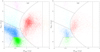 |
Fig. 1 Gaia-2M diagram for the LMC and SMC (models 1 and 2). Boxes and colours indicate the various classes according to Lebzelter et al. (2018) and Mowlavi et al. (2019). |
3 Model
The studies using the JAGB method mentioned in Sect. 1 highlight that no standard method has yet been developed to determine the absolute J magnitude. Authors have used the mean, the median, and the mode, have fitted Lorentzian and Gaussian functions, and have applied different ranges in J − Ks, and sometimes in the J magnitude as well. All these methods are explored below.
One fitted model is a Gaussian plus a quadratic function (Zgirski et al. 2021)
 (4)
(4)
where x refers to the J magnitude, N is a scaling number, µ is the sought-after absolute magnitude, σ is the width, b, c, and d represent the background terms (taking into account any contaminants of the sample of carbon stars), and xo is a constant chosen to be −6.2 mag. The second fitted model is a modified Lorentzian profile introduced by Parada et al. (2021), and, adding the background terms, our implementation reads
 (5)
(5)
where µ is the sought-after absolute magnitude, w is the width, s is the skewness, and k is the kurtosis of the distribution. The fitting is done with the Levenberg-Marquardt algorithm (the routine mrqmin as implemented in Fortran by Press et al. 1992).
4 Results
4.1 Magellanic Clouds
In a first step, the results of a standard model are presented, where stars are selected in a box of 1.3 < (J − Ks)0 < 2.0 mag and −5.0 < (MJ)0 < −7.5 mag. C stars are selected (i) as those that are C stars according to the Gaia-2M diagram and (ii) based on the classification in the LPV2 catalogue. No background terms are included in the fitting (Eqs. (4) and (5)). Figure 1 shows the Gaia-2M diagram, Fig. 2 the K0 − (J − Ks)0 CMD, and Fig. 3 the fit to the J-band LF of stars in the box for the LMC and SMC (models 1 and 2), respectively. Results of the fitting are listed in Tables 1, B.1 and B.2, which give general results, the results from fitting the Gaussian model, and the results from fitting the Lorentzian model, respectively. The latter two tables list the reduced χ2  and also the value of the Bayesian information criterion (BIC, Schwarz 1978). This is a useful parameter for deciding whether or not the lower χ2 expected for models with more parameters is significant.
Tables 1, B.1 and B.2 include several fitted models, starting with the standard model (models 1 and 2 for for LMC and SMC, respectively)7. The first parameter to vary is the lower limit of the selection box (models 3–8). Visually, a smaller lower limit would encompass more of the SMC C stars, while a larger lower limit one is more suitable for the LMC. With a lower limit of 1.2 in (J − Ks)0 the contamination of O-rich stars is 13% for the SMC and 34% for the LMC. For a lower limit of 1.5 in (J − Ks)0, these values are 4% and 1%, respectively. Another interesting parameter is the slope of (MJ)0 versus (J − Ks)0 of the stars inside the selection box. This slope increases (from negative to zero to positive) when increasing the lower limit of the selection box. The CMD indicates why this is the case, namely because contaminants inside the selection box occur at fainter and bluer magnitudes than the typical C star. A non-zero slope indicates that the distribution of stars is not symmetric around (MJ)0, as assumed in fitting a Gaussian distribution. Indeed, the fitted models indicate that a Gaussian distribution is a poor fit to the LF of the LMC C stars (comparing models 1 with 13 for the LMC, and models 2 and 14 for the SMC). The Lorentzian distribution clearly gives a the better fit than a Gaussian distribution. Adding the background terms marginally improves the  in the case of the Lorentzian distribution, but the BIC values are larger indicating that the data does not require the addition of these terms. In the case of the Gaussian distribution the BIC values are smaller when including the background terms. Adding the background terms could also influence the fitted values for the width of the Gaussian profile, as well as the width, skewness, and kurtosis of the Lorentzian profile. Models 23 and 24 for the LMC are similar to models 3 and 7 (with the lower limits of (J − Ks)0 of 1.2 and 1.5 mag, respectively), but include the background terms. The effect on the fitted parameters are largest for the bluest lower limit on (J − Ks)0, where the contamination of M-stars is largest. The BIC values are lower when including the background terms, but the effect is marginal for the model fitting the Lorentzian profile, which results in the lowest BIC value. Purely in terms of fitting the LF, the Lorentzian distribution is best, followed by the Lorentzian plus background terms, the Gaussian distribution plus background terms, and the Gaussian distribution.
The consequence of adopting the Lorentzian distribution is the conclusion that the LMC and SMC LF are different, as already concluded by Parada et al. (2021, 2023). These authors use a lower limit of (J − Ks)0 > 1.4 mag (our models 5 and 6). The parameter values are similar and the trends identical, namely the mode and the skewness of the LMC and SMC distributions are significantly different. In terms of calibration, Parada et al. (2021, 2023) propose to take the LMC as a calibrator if the skewness of the distribution in the target galaxy is <−0.2, otherwise taking the SMC. Based on models 1−8, the results in the present paper put this value for the skewness at −0.10. Alternatively, one could assume and adopt a linear relation between the skewness and the mode, and estimate the mode based on the skewness of the LF in the target galaxy.
The conclusion in the papers by Madore, Freedman, and coworkers is that the mean magnitude of the selected SMC and LMC stars is very similar, and can be averaged to a single value that can be applied to any target galaxy. The results of the present analysis confirm this. Considering models 1−8, which vary the most important parameter, namely the lower limit to the (J − Ks) colour, and considering all stars in the selection box, the weighted difference in the weighted mean magnitudes between LMC and SMC is −0.025 ± 0.007 mag, and this is smaller (in absolute sense) than the weighted difference in the median magnitudes of −0.066 ± 0.005 mag, or the weighted difference in the peaks of the Gaussian distribution of −0.031 ± 0.007 mag. In the present paper, we introduce also another approach, namely to fit a linear relation between the dereddened absolute J magnitude and the ((J − Ks)0 − 1.6) colour to all stars in the selection box. The average difference in the zero points (ZPs) between LMC and SMC is even smaller at −0.016 ± 0.006 mag.
Therefore, averaging the weighted mean magnitudes or the ZPs of the LMC and SMC (models 1−8) gives a weighted mean of −6.212 mag with a rms of 0.021 mag, and a total error that is driven by the systematic error in the adopted DM to the LMC and SMC (cf. Freedman & Madore 2020).
The parameters were fitted based on all stars in the selection box, with the underlying assumption that these are, for the most part, C stars. In typical applications, the selection is purely a photometric one with no a priori knowledge of the spectral type. The average difference between models 1−8 in terms of the weighted mean of all stars minus the weighted mean of the C stars is +0.010 mag, with an error on the mean of 0.002 mag and a rms of 0.012 mag. This means that C stars are on average slightly brighter than the average star in the selection box, as expected, as the contaminants come mostly from fainter (and bluer) stars. The way the C stars are selected (models 1−2, 17−22) plays a minor role. The rms in the weighted average is 0.010 mag.
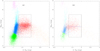 |
Fig. 2 CMD for the LMC and SMC (models 1 and 2). Colours correspond to the classes in the Gaia-2M diagram. The black box indicates the stars selected to construct the J-band LF. The blue line indicates a linear fit to all stars inside this box. |
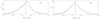 |
Fig. 3 Fit to the J-band LF (models 1 and 2). The red and black histograms refer to the C stars and all stars, respectively. The bin width is 0.05 mag. The dark and light-blue lines refer to the best-fit Gaussian and Lorentzian profile of the C star LF, respectively. The vertical black and red lines refer to the weighted mean and the median (MJ)0 magnitudes of the C stars in the selection box, respectively. |
General results.
4.2 Milky Way
The results for the MW turn out to be less straightforward to interpret than those for the MCs. Model 101 in Tables 1, B.1 and B.2 used the same selection box as the standard model, but background terms were included, and some terms in the fitting were fixed to achieve convergence (the width of the Gaussian and the Lorentzian distribution were set to the average found for LMC and SMC, and the skewness and kurtosis were set to zero). A feature of the MW models is that absolute magnitudes are calculated from individual distances with errors and that an error in the DM σDM < 0.2 mag was adopted. The Gaia-2M, a CMD, and the fit to the LF are shown in Fig. 4.
Several points are immediately clear. The number of stars in the selection box is small, smaller even than for the SMC, and the contamination by O-rich stars is close to 50%. This high level of contamination is also clear from the CMD and from the LF. The mean, median and the peak of the Gaussian and Lorentzian distribution differ significantly from that found for the MCs. The CMD and Gaia-2M diagram for the MW are also qualitatively different from those for the MCs with fewer bright stars present. Increasing the lower limit in the (J − Ks) and MJ colour of the selection box reduces the level of contamination (model 102, bottom panel in Fig. 4), but the magnitudes do not change significantly.
Figure 5 shows the cumulative number of all stars as a function of distance. The closest star in the selection box is found to be at about 1.4 kpc (and the closest C star is at about 1.7 kpc). The figure also shows some theoretical models that indicate that the selected subsample is incomplete beyond about 2.8 kpc.
That the closest AGB star in the sample is only at 1.4 kpc is surprising. For example, Andriantsaralaza et al. (2022) determine distances to 201 AGB stars (of which 188 are within 1.4 kpc) and only one is present in the MW sample. We note, however, that only 5 of the 201 objects have an ‘AAA’ photometric flag in 2MASS (they are located at 4.0, 1.5, 1.1, 1.0, and 0.6 kpc, respectively), and the others have quality flags signalling lower-quality NIR data, which in almost all cases is because the sources are very bright. Three of the five stars do not obey σπ/(π + 0.1) < 0.2, and one is not listed in the LPV2 catalogue. As another example, of the 258 stars in Whitelock et al. (2006), 220 have a 2MASS counterpart (within 6″), but only 113 have a quality flag of ‘AAA’. Of those, 11 do not have a parallax listed in the Gaia catalogue, 44 do not obey our parallax selection criteria, and 3 are not listed in the LPV2 catalogue. Therefore, in this case, only 55 out of 258 stars are in the MW sample. It is clear that the MW sample is incomplete for nearby AGB stars, primarily because 2MASS magnitudes are unreliable for bright stars, and secondly because of the relatively poor parallax determinations, which is a particular problem for AGB stars and red supergiants as convection-related surface dynamics leads to photocentre shifts that impact the accuracy of the parallax determination (e.g. Chiavassa et al. 2018, 2022).
To remedy this, (1) we considered nearby AGB stars with NIR photometry other than from 2MASS, (2) for AGB stars in OCs, we replaced the Gaia parallax of the AGB star by the more accurate parallax of the host cluster, and (3) we searched for wide binary systems (WBSs) where the companion to the AGB star has a more accurate parallax.
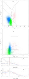 |
Fig. 4 Results for model 101 in the top three panels: the Gaia-2M diagram, the CMD, and the LF. Bottom panel: the LF for model 102. |
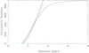 |
Fig. 5 Cumulative number of stars in the selection box. Coloured lines indicate model predictions (Groenewegen et al. 1992, Eq. (20)) for a volume density (ρ0) of 70 /kpc3 and scale height H = 200 pc (red), ρ0 = 28/kpc3 and H = 500 pc (dark blue), and ρ0 = 14/kpc3 and H = 1000 pc (light blue). The expected number of stars inside approximately 1.4 kpc is subtracted (158, 132, and 95 stars, respectively). |
4.2.1 Adding MW stars with SAAO photometry
Regarding the first strategy, we added AGB stars (of all spectral classes) from a variety of papers with photometry on the SAAO system. The advantage of using photometry this system is that a significant set of data with homogeneous photometry is available. The following data sets were considered: 239 C stars, 19 CS stars, and peculiar and uncertain C stars from Whitelock et al. (2006), 193 Mira and semi-regular variables that were observed by HIPPARCOS from Whitelock et al. (2000), 161 late-type stars in the South Galactic Cap from Whitelock et al. (1995), and 61 Miras in the South Galactic Cap from Whitelock et al. (1994). The combined list has 644 unique entries. The photometry is taken from the most recent work in case of multiple entries. An additional advantage of this data set is that the reported magnitudes do not result from single-epoch observations, but are the mean magnitudes derived from a Fourier analysis of the light curves.
This list of sources was treated in the same way as before, that is, it was correlated with Bailer-Jones et al. (2021) and the various Gaia catalogues, and the STILISM tool was used to obtain the reddening. Initially, the SAAO photometry was transformed to the 2MASS system using Eq. (1) in Koen et al. (2007) but further investigation led us to derive transformation equations specific to the present sample, as outlined in Appendix C.
This procedure results in transformed SAAO data for 475 objects, while this was not possible for 169 objects, which were either not listed in Gaia (mostly because the stars are so red that they are expected to be far fainter than G = 21), are listed in Gaia but without a parallax (solution_type= 3) or the parallax accuracy is too poor (Rplx < 5), or they are not listed in the LPV2 catalogue. Of the 475 objects, 147 were already in the MW sample. They are not removed as the photometry is determined independently. Only 152 of the 475 stars are classified as C-star in the LPV2 catalogue.
Model 103 extends model 102 by including this additional sample of stars. Figure F.2 shows the cumulative number of all stars as a function of distance and indicates that the number of nearby stars has increased significantly, although it is clear that the sample still is far from volume complete8. However, the total number of C stars inside the selection box that fulfil all criteria is only increased by 38. On average the absolute magnitudes are slightly brighter. A model where the width of the Gaussian and the Lorentzian distribution are fitted does converge now, but with large error bars in these parameters, and its results are not listed explicitly.
4.2.2 AGB stars in OCs
Regarding improved distances for AGB stars in OCs the list of stars and clusters in Tables 1 and 2 from Marigo et al. (2022) were considered (excluding the cases listed as doubtful), which results in 51 unique objects. In those tables distances based on GDR2 data (from Cantat-Gaudin et al. 2020) are listed. In their Appendix, Marigo et al. (2022) recompute the cluster parallaxes using GDR3 data and considering various PZPOs, but only for a limited set of clusters. Therefore, we decided to compute OC parallaxes from GEDR3 data for all clusters; see Appendix D for details. Correlating the position of the AGB stars against the 2MASS catalogue, and retaining only stars with quality flag ‘AAA’ results in 22 matches in 18 clusters. All but one were already in the MW sample. One extra object was found as the initial selection was now relaxed to Rplx > 1, anticipating that the cluster parallax is more accurate than the individual parallax. This source was added to the MW sample, and for the remaining 21 stars the individual parallaxes were updated with the cluster parallax from Table D.1. Only 8 are classified as C-stars in the LPV2 catalogue.
These changes are implemented in model 104. The number of stars that fulfil the criteria is only marginally increased compared to model 103 (many of the stars are too blue) and the results have hardly changed.
4.2.3 Looking for common-proper-motion companions
One additional way to obtain improved parallaxes for AGB stars is to use the parallax of a physical companion in a WBS. Initially the catalogue of El-Badry et al. (2021) – with over a million WBSs – was queried, but as a parallax lower limit of 1 mas is imposed in their work, it was deemed necessary to perform an independent search as most of our objects are located beyond 1 kpc. To keep a useful and manageable subsample, only the approximately 20 800 objects with 1.3 < (J − Ks)0 < 2.0 mag were considered. To test the scripts and codes an equally sized test sample was selected from El-Badry et al. (2021), for which the parallaxes of the primaries and secondaries are close to their limit of 1 mas. Details of the procedure are given in Appendix E and a total of 65 candidate WBSs were found. For those objects, the parallax, parallax error, goodness-of-fit GoF, RUWE, and distances from Bailer-Jones et al. (2021) were updated with those of the candidate WBS. These changes are implemented in model 105. Again, the number of objects only marginally increases and the results remain unchanged.
4.2.4 Final remarks and models for the MW
Of the different procedures used to increase the number of C stars with accurate distances inside the selection box, the inclusion of nearby stars with SAAO photometry proved to be the most efficient. Using AGB stars in OCs or in WBSs had very little effect. Indeed, it added more O-rich stars in proportion, and the contamination rose from 12% (model 103) to 19% (model 105). In model 106, the lower limit of the selection box is set to (J − Ks)0 = 1.5 mag, and the contamination of O-rich stars is reduced to 9.5%.
Above, no selection on the quality of the astrometric solution has been taken into account. However, many solutions are poor with GoF (or RUWE) parameters outside the recommended range; see e.g. Table E.1. In model 107, only sources with −4 < GoF < 10 were kept, which reduced the number of selected sources by one-third compared to model 106.
Another potential issue is the adopted reddening. In a significant number of cases, the estimated distance is larger than the largest distance (dmax) available in the 3D reddening map. In all previous MW models, the adopted reddening in such cases was the reddening at dmax, which implies an underestimate of the true reddening. In model 108, the only stars that are kept are those for which the estimated distance is less than 1.5 · dmax, and this reduces the number of stars in the final sample by about 55%. An alternative is model 109, where the E (B − V) is simply scaled with d/dmax, which certainly leads to an overestimate of the reddening.
Finally, we used updated reddening maps of Lallement et al. (2022) and Vergely et al. (2022)9, which typically go out to larger distances than the STILISM maps, although these latter only became available when the present work was close to completion. However, for technical reasons this proved practically impossible to do for all of the 250 000 stars in our sample, and updated reddenings and corresponding values for dmax were only obtained for the approximately 21 300 stars with 1.3 < (J − Ks)0 < 2.5 mag that could reasonably make it into the selection box. Model 110 contains the results with the updated reddenings, again only retaining stars where the estimated distance is less than 1.5 · dmax. In model 111 E(B − V) is again scaled with d/dmax, with the additional limit that AV < 1.5 mag. Limiting the sample to the most accurate distances (σDM < 0.1 mag) results in few stars, where the Gaussian and Lorentzian fits become meaningless (model 112). Model 113 is a model without background terms (the BIC decreases successively when setting d, d+c, and d+c+b to zero, respectively) and with limits -5.2 < (Λfj)o < -6.2 mag, approximately centred around the fainter magnitude of the MW stars.
In the models presented so far, the widths of the Gaussian and Lorentzian distributions are fixed to the typical values found for the SMC and LMC. However, Ripoche et al. (2020) found a width in the LF of the MW that was much larger than in the MCs. In model 114, the widths of the Gaussian and Lorentzian distributions have been fixed to 0.6. The change in the peak magnitudes (~0.02 mag) is much smaller than the error in the peak magnitudes (~0.09 mag).
Although there are uncertainties due to the adopted reddening, the quality of Gaia’s astrometric solutions, and the accuracy of the parallaxes, models 106 to 114, with a selection of 1.5 < (J − Ks)0 < 2.0 mag and a contamination by O-stars of less than 10%, are consistent in that they lead to absolute magnitudes in the MW that are systematically fainter than in the MCs by about 0.2–0.4 mag. However, the scatter in the fitted absolute magnitudes due to these different assumptions is of order 0.1 mag, and is much larger than for the MCs.
4.3 Recommended models for calibration
We present the final models that are recommended for calibration. They are driven by our results regarding the MW, although these results remains puzzling; see Sect. 5.
The models assume 1.5 < (J − Ks)0 < 2.0 mag and a box length in J magnitude of ∆(MJ)0= 1.2 mag. No background terms are included. C stars are selected as those that are C stars according to the Gaia-2M diagram or according to the classification in the LPV2 catalogue. For the MW, the model includes updated parallaxes for AGB stars in OCs and WBSs and nearby stars with SAAO photometry transformed to the 2MASS system, only retaining solutions with −4 < GoF < 10, updated reddenings from Lallement et al. (2022) and Vergely et al. (2022), scaling the reddening with the distance relative to dmax, and imposing AV < 1.5 mag and σDM < 0.2 mag.
These are models 25 (LMC), 26 (SMC) and 115 (MW), and the relevant figures are displayed in Fig. F.3. Table 2 compares the results obtained in the present work with values in the literature.
So far in the present work the statistical errors quoted are the errors on the mean. To obtain a different estimate of the error bar, we performed Monte Carlo simulations where the analysis was repeated 1001 times on datasets where the J and K-band magnitudes, the E(B − V) reddening, and the distance were varied according to Gaussian distributions. The second line in Tables 1– 2 for models 25, 26, and 115 give the 50th percentile and half the difference between the 84th and 16th percentiles as error. The error bar calculated in this way can be either larger or smaller than the formal error on the mean depending on the galaxy and the fitted parameter.
For the MCs our final results are largely in agreement with previous estimates in the literature. The (MJ)0 is slightly brighter in the LMC than in the SMC, regardless of which estimator is used. The smallest difference between the two is when using the ZP at J − Ks = 1.60 mag, followed by the (weighted) mean magnitude. As done by Madore & Freedman (2020) and Freedman & Madore (2020), one can therefore argue that the values for the LMC and SMC can be averaged and that they are consistent with a weighted mean value of −6.212 ± 0.021 mag based on our models, which is marginally brighter than the −6.20 adopted by Madore, Freedman and collaborators.
The same is true when considering a measurement based on the peak value of a Gaussian fit. On the other hand, it is clear that a Gaussian does not provide a good fit to the LF and so one might question the meaning of the fact that the peak values agree. When considering a Lorentzian function, the LF is well fitted, but then one has to conclude that the LF and peak values are different in the SMC and LMC, and we essentially confirm the results in Parada et al. (2021, 2023).
The results for the MW remain puzzling. We find a fainter value for (MJ)0 than in the MCs; the value we find is in between those of Ripoche et al. (2020) and Madore et al. (2022). The former authors used Gaia DR2 parallaxes, and a colour cut with a lower bound at J − Ks = 1.40 mag, which should have a larger fraction of contamination by O-rich stars. The preferred average quoted in Madore et al. (2022) is based, on the one hand, on AGB stars in OCs where a lower bound of J − Ks = 1 .2 mag is used and a sample that is known to contain only few confirmed C stars and in fact known non-C stars, and, on the other hand, on a sample of C stars of which the majority have very poor 2MASS photometry.
Results on the JAGB method.
5 Discussion and conclusions
The main purpose of the present paper is to consider the influence of contamination by O-rich AGB stars on the absolute J-band magnitude in a colour-magnitude box selected to contain (predominantly) C-rich stars. The blue limit in (J − Ks)0 colour is the main driver behind this contamination. For the MW a limit of 1.5 is required to have a contamination of <8% (in model 115). In the MCs, the level of contamination is negligible for such a limit. We determined the mean, median, and the peak of Gaussian and Lorentzian profile fits. Imposing a range in J (or MJ) of 1.2 mag also reduces the contamination and ensures that no background terms are required to fit the Gaussian and Lorentzian profiles. In practise, this means that iterations may be required. For an initial guess of the DM to an external galaxy, the range in J magnitude can be determined (or no limit is imposed in the first iteration) after which the mean, median, Gaussian, Lorentzian values are determined, and then a new range in J can be applied.
The values we find for (MJ)0 are in agreement with the literature for the SMC and LMC. The two methods proposed in the literature for distance determination both seem plausible. The LFs of the SMC and LMC are different, and so could alternatively use a calibration depending on the skewness of the distribution (a ‘LMC-like’ and ‘SMC-like’ calibration). On the other hand, for the SMC and LMC, the mean magnitudes inside the colour selection box agree to within the errors and so an average value is formally an accurate mathematical representation.
Our result for the MW is puzzling. A fainter value is found, contrary to theoretical model predictions. Eriksson et al. (2023) calculated synthetic photometry for C-stars based on radiation-hydrodynamics simulations of the dust formation for a grid of models with solar composition (with different values for the C/O ratio). In their Fig. 17, these authors show the MJ versus (J − K) diagram and note a ‘general similarity to Fig. 1 in Madore et al. (2022)’. However, this figure suggests that in the range 1.4 < (J − K) < 2 mag, MJ depends on (J − K). Using the data in Eriksson et al. (2023) for the models with 1.4 < (J − K) < 2 mag Table 3 lists the median MJ and the median absolute deviation (MAD) as a function of stellar mass10. As expected, higher-mass C-stars have a brighter J-band magnitude, indicating that the SFH of a galaxy should also influence the average magnitude of C-stars. The effect of metallicity for a given initial mass appears to be small. For a 2.5 M⊙ star, the maximum luminosity attained during the C-star phase is L = 13 000, 10 000, 9400, and 9000 L⊙ at Z = 0.001, 0.004, 0.008, and solar metallicity, respectively (P. Ventura, private communication, see e.g. Dell’Agli et al. 2015). In this case, larger metallicity tends to indeed give lower maximum luminosity, and in terms of bolometric magnitude this corresponds to a change of about 0.12 mag from SMC to solar metallicity. For lower initial masses, the trend with metallicity is less clear and the effect is weaker. The straight comparison of the bolometric luminosity ignores the effect of mass loss and effective temperature on the NIR magnitudes. Preliminary models using the PARSEC-COLIBRI tracks (Marigo et al. 2017) including TP-AGB evolution with mass loss (Pastorelli et al. 2019, 2020) and the population synthesis code TRILEGAL (Girardi et al. 2005) indicate that in the age range of 0.63–1 Gyr for Z in the range 0.006 to 0.014 (corresponding to about 2.2–2.5 M⊙ initial mass), the average J-magnitude during the C-star phase becomes brighter by about 0.4 mag (Pastorelli et al., in prep.). At solar metallicity, this average is about MJ ~ −6.8 mag for a star of nearly 2 M⊙, which is in reasonable agreement with the model by Eriksson et al. (2023).
The situation is complex from an empirical point of view. Reddening possess a challenge, but putting limits on the maximum reddening does not have a large impact. We also ran a model with the selective reddening of Wang & Chen (2019) replaced with that of Cardelli et al. (1989). This made the absolute magnitudes brighter, but only by ~0.02 mag. A larger change (~0.1 mag brighter to near −6.0 mag) occurred when not using the distance estimate by Bailer-Jones et al. (2021) but the reciprocal of the parallax instead. This gave a still fainter magnitude than one might expect but possibly reflects the two assumptions in Bailer-Jones et al. (2021). The first is that a prior is used in Bailer-Jones et al. (2021) based on a mock Gaia catalogue that includes all objects. This prior may not be optimally suited for AGB stars (see Andriantsaralaza et al. 2022). Also, as the parallaxes of AGB stars are more uncertain than those of non-AGB stars of comparable magnitude and colour, the prior has a larger influence on the a posteriori distance estimate. Second, Bailer-Jones et al. (2021) used the PZPO correction of Lindegren et al. (2021). There is ongoing debate as to whether this PZPO is too small or rather over-corrects and is too large; see e.g. Figure 10 in Molinaro et al. (2023), or Groenewegen (2024). Ninety percent of the stars in the final MW sample have G magnitudes in the range of 7.0–11.5 mag, and (Bp − Rp) colours that range from 2.4 to 3.9−6.3 mag for the reddest 10%. The PZPO is very poorly known in this regime, and, for example, Cruz Reyes & Anderson (2023) in their study of Cepheids in clusters even entirely exclude this magnitude range and colours redder than 2.75 mag.
For an unbiased absolute calibration, a volume-complete sample would be best. The major obstacle in achieving this is the lack of reliable 2MASS photometry, as the most nearby AGB stars saturate. Due to the large year-long effort, there is a substantial number of AGB stars with SAAO photometry, but the sample is still incomplete. A dedicated effort to obtain NIR photometry for a few hundred (C- and O-rich) AGB stars in both hemispheres with good Gaia astrometric solutions, and with suitable (J − K) colours, and that saturate in 2MASS, would be beneficial for an improved calibration in the future. This would only require relatively small telescopes. A complementary approach is to study the JAGB LF in other galaxies with solar-like metallicities and this is work in progress.
Results of the models by Eriksson et al. (2023) for a solar composition.
Data availability
Appendix F is available at http://doi.org/10.5281/zenodo.14008075.
Acknowledgements
EM would like to thank Martin Groenewegen for making this internship in the Royal Observatory of Belgium possible, allowing me to do this research. I am grateful for his helpful comments and tips, and for the coffee at noon with his colleagues. The authors thank the referee for a thorough report that has improved the paper. This research was supported by the International Space Science Institute (ISSI) in Bern, through ISSI International Team project #490, SHoT: The Stellar Path to the Ho Tension in the Gaia, TESS, LSST and JWST Era”. In particular the very generous extension of the stay by one day related to the strike of the German railroad in December 2023 is highly appreciated by MG. We thank Dr. Katie Hamren and Dr. Steve Goldman for providing their catalogues with spectral classifications and Dr. Greg Sloan for comments on the paper. This work presents results from the European Space Agency (ESA) space mission Gaia. Gaia data are being processed by the Gaia Data Processing and Analysis Consortium (DPAC). Funding for the DPAC is provided by national institutions, in particular the institutions participating in the Gaia MultiLateral Agreement (MLA). The Gaia mission website is https://www.cosmos.esa.int/gaia. The Gaia archive website is https://archives.esac.esa.int/gaia. This research has used data, tools or materials developed as part of the EXPLORE project that has received funding from the European Union’s Horizon 2020 research and innovation programme under grant agreement No 101004214. This work makes use of data products from the Two Micron All Sky Survey, which is a joint project of the University of Massachusetts and the Infrared Processing and Analysis Center/California Institute of Technology, funded by the National Aeronautics and Space Administration and the National Science Foundation. This research has made use of the VizieR catalogue access tool, CDS, Strasbourg, France.
Appendix A Radial velocities
Of the 4973 and 39014 stars in the SMC and LMC sample, 1400, respectively, 17731 have an RV listed in the main Gaia catalogue. Fig. A.1 shows the distribution in RVs, which are consistent with the expected values, indicating that the selection on position, parallax, and proper motion result in reliably selected MC samples.
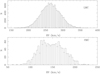 |
Fig. A.1 Radial velocity distribution of SMC and LMC stars selected on position, parallax, and proper motions. |
Appendix B Additional tables
Results of the Gaussian fit.
Results of the Lorentzian fit.
Appendix C Transformation from SAAO to 2MASS photometry
Initially, the SAAO photometry (dereddenned) was transformed to the 2MASS system using Eq. 1 in Koen et al. (2007). For the 147 stars that were also in the original MW sample it was possible to compare the 2MASS photometry to the transformed SAAO photometry. Taking J as example the median difference was 0.005 mag but the largest differences were more than a magnitude in some cases. A closer inspection revealed that this was primarily so for the reddest sources. They were outside the validity range of the transformation formulae that are −0.043 < (J − H) < 0.992, −0.087 < (J − K) < 1.390, and −0.044 < (H − K) < 0.503 (Koen et al. 2007). The differences were also larger for sources where the trimmed_range_mag_g_fov (IQR5) was large, suggesting the effect of variability. Restricting the comparison to (J − K) < 2.0 and IQR5 < 1 mag (non-Mira variables), the median difference of J was −0.015 and for 60 of the 63 sources the absolute difference was 0.21 mag or less. In K these numbers were +0.037 and 0.17 mag, respectively.
In a next step the original SAAO photometry was directly compared to the 2MASS photometry (for sources with quality flag ’AAA’) for 160 sources. This sample was slightly larger as the condition that the star was in the LPV2 catalogue was not imposed. The condition on the parallax error was imposed in order to have a distance estimate from Bailer-Jones et al. (2021) so that the reddening could be estimated. In JAGB method a limit on (J − K) is used and therefore the same limit is imposed in deriving the transformation formula. To limit the influence of variability a limit on the absolute difference between the magni-tudes is imposed following Figs. 4, 5, and 6 in Koen et al. (2007). Figure C.1 shows the results which are typically based on 55-60 stars.
In J the derived slope was formally not significant but agrees with Koen et al. (2007) and the adopted formula is
 (C.1)
(C.1)
with an rms of 0.043 mag.
In the H-band the slope was not significant
 (C.2)
(C.2)

was adopted, as in Koen et al. (2007).
In the K-band the derived slope was significant and the transformation formula was
 (C.4)
(C.4)
with an rms of 0.060 mag.
After applying these formula the comparison of the 2MASS to the transformed SAAO photometry restricted to (J − K) < 2.0 and IQR5 < 1 mag (non-Mira variables) gives a median differ-ence in J of −0.001 mag and for 60 of the 63 sources the absolute difference was 0.19 mag or less. In K these numbers were +0.007 and 0.22 mag, respectively.
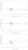 |
Fig. C.1 Difference between 2MASS and SAAO photometry in JHK against SAAO (J − K) photometry. The black lines represent the formal fit (see text), and the blue line the result from Koen et al. (2007). In the K-band the latter is not plotted as the transformation formula in Koen et al. (2007) depends on (H − K) and (J − H). |
Appendix D Cluster parallaxes
Cluster parallaxes are a way to improve upon the parallax of individual AGB stars that are in open clusters. Marigo et al. (2022) re-investigated the population of AGB stars in Galactic OCs using Gaia data. These authors presented results mainly based on GDR2 data and an update using GDR3 data was only performed for a subset of clusters. An independent analysis of the cluster parallaxes is presented here, largely following Marigo et al. (2022). Full details on the analysis and for a much larger set of clusters will be presented elsewhere (Groenewegen, in prep.).
For the clusters analysed here (and in Marigo et al. 2022) cluster members and cluster membership probabilities were taken from Cantat-Gaudin & Anders (2020). A dedi-cated script and Fortran code was used to do the analysis. The list of members was read and the GDR3 main cata-logue queried on position (the DR2 position) using a search radius of 0.15″, and various quantities were retrieved, like the source_id, the parallax and error, the astrometric_gof_al (GoF) and RUWE quality flags, the G, Bp and Rp magnitudes, the non-single star (NSS) flag, the galactic end ecliptic coordinates, and the astrometric_params_solved, nu_eff_used_in_astrometry, and pseudocolour flags.
Marigo et al. (2022) presented results using (i) no PZPO and using the prescriptions in (ii) Lindegren et al. (2021) (hereafter L21) and (iii) Groenewegen (2021) (hereafter G21). As the dis-tances in the MW sample were by default based on Bailer-Jones et al. (2021), that uses the L21 correction, only that correction was considered here. In a first pass the median value and standard deviation (calculated as 1.4826 × MAD) of the GoF and parallax were calculated. In a second pass the final sample was selected. Stars with  were excluded, as well as stars with a GoF less than −3.5, or larger than the median value + 3 times the standard deviation (with a minimum of +3.5), stars with a nonzero NSS flag, and stars with a membership probability <0.5. Stars were also restricted to the range 0.15 < Bp − Rp < 3.0 to stay within the validity range of the L21 correction.
For this sample the weighted mean parallax (including the L21 correction) and error in the mean was calculated, as well as the median parallax and the standard deviation. The error in the mean was typically very small, but one has to take into account the angular correlation in the parallax (e.g. Vasiliev & Baumgardt 2021) and this sets the floor to the accuracy that can be achieved. To estimate this effect the distance between all members was calculated and the spatial correlation calculated according to Vasiliev & Baumgardt (2021), and the error was then taken as the median value over all pairs.
Finally the finite size of the cluster was taken into account as the position of any given member is unknown. To estimate this effect the distance between any member and the centre of the cluster (itself taken as the median in right ascension and decli-nation) was calculated, and the 68% percentile was taken as the typical size. This angular size on the sky was converted to a line-of-sight change in parallax assuming a sphere. This effect was negligible apart from a few large, nearby clusters.
The results are compiled in Table D.1 where the cluster parallax and its final error are listed as well as the different com-ponents to this error bar, the size of the cluster and the number of selected members. In almost all cases the error bar is set by the limit due to the spatial correlation. For comparison, the val-ues in Marigo et al. (2022) are listed in the format of the original paper, that is, quoting the 68% confidence intervals. Marigo et al. (2022) appear to quote the standard deviation and in column 8 their and our values are compared directly and the agreement is excellent, typically to 0.01 mas or better, except in a few clusters with few members, and where the results may depend on details in the selection of the final sample.
Cluster parallaxes.
Appendix E Wide-binary systems
In this section the search for candidate WBSs is outlined, which largely follows the procedure in El-Badry et al. (2021) (hereafter E1B21). To test the procedure described below a test sample of similar size was selected from the ElB21 catalogue with paral-laxes close to 1 mas (as the AGB stars are typically at larger distances). Of the two stars the one with the larger parallax error was taken as the target star.
We first describe the procedure followed for the test sam-ple, and then indicate the changes made for the AGB sample (which are stricter). Following ElB21, all objects within 1 pc (or 206.3 kAU) were selected using (π + σπ) of the target star to convert physical distance to angular distance. All objects within this angular distance of the target object were selected from the Gaia main catalogue. Following ElB21, a limit Rplx ≥ 5 was imposed. One can define a χ2 statistic
 (E.1)
(E.1)
for the parallax, where the subscript t refers to the target and WBS to the WBS candidate, and similarly, χ2 statistics for the proper motion (PM) in RA and the PM in Declination. Following ElB21, an initial limit  was imposed. ElB21 does not impose limits on
  and
and  but this is done here. In the case of the test sample they are very generous and have no impact on the results (
 and
and  ). The output of this first step are the parameters of the candidate WBSs for each target. Using these selection criteria counterparts are found for 99.8% of the targets in the test sample. At this point there can still be multiple candidate WBSs
In a second step, additional criteria were employed, and a single WBS candidate was determined. Requiring that all can-didate binaries have proper motion differences within 3σ of the maximum velocity difference expected for a system of total mass 5 M⊙ with circular orbits leads to the condition (El-Badry & Rix 2018; El-Badry et al. 2021)
 (E.2)
(E.2)
where the quantities ∆µ, ∆µorbit, and σµ are calculated following Eqs. 4, 5, and 6 in El-Badry & Rix (2018). In addition, ElB21 impose
 (E.3)
(E.3)
where f= 6 for separations less than 4″ and f= 3 otherwise.
If an object obeys Eqs. E.2, Eqs. E.3 and the physical separation (= angular separation in arcsec/  ) was less than 206 kAU the object was considered as a valid WBS candidate.
If there was more than one candidate an additional selection step was required. El-Badry et al. (2021) does not discuss this situation in detail, and the following procedure was devised in order to retrieve the correct counterpart as listed in ElB21 in the overall majority of cases. A total  was calculated based on the χ2 in parallax and the two PM components.
 (E.4)
(E.4)
A selection on  was imposed. However, the retrieval of the correct counterpart was increased by adding more weight to the χ2 in parallax. In the case of multiple candidate counterparts the one listed by ElB21 was almost always the one closest to the target, even if it did not have the lowest χ2 in our analysis. In the end, the candidate WBS is the one with the smallest value of χ2,
 (E.5)
(E.5)
where P is a penalty function which favours counterparts closer to the target, P = 12⋅ (d/300″)2, where d is the distance between the target and the WBS candidate in seconds of arc.
With these procedure, of the 21600 objects in the test sample, 14400 have a single WBS candidate (in all cases the one listed by ElB21), and in the 7200 cases where there were multiple candidates the one listed by ElB21 is picked in 99.8% of the cases. The remaining 15 cases were checked in detail, and the WBS compo-nent found by our procedure is equally, or more, likely than the one listed in ElB21. As briefly mentioned by them, the target star can be in a multiple system and the procedure may ultimately find another WBS candidate that is part of the same hierarchical system.
For the AGB sample, slightly stricter criteria have been adopted in step 1. Objects with solution_type= 3 were excluded (i.e. objects without parallax in the Gaia catalogue. This is not relevant for the test sample). The physical distance limit was (somewhat arbitrarily) reduced to 65 kAU, to lower the probability of a change alignment. With this limit the likely common-proper motion component around R Scl was retrieved (at 159″ on the sky, see below). Stricter limits were used on the PMs,  and
and  . It was imposed that the errors in the parallax and the two PM components are smaller in the WBS candidate than in the target star as the hypothesis is that these errors are larger in the target star simply because of its very AGB nature. Applying the criteria in step 1 and step 2, 65 candidate WBS were found, and they are reported in Table E.1
Possibly the most interesting specific result is the discovery of candidate companions to R Scl (2.703 ± 0.017 mas) and R Hya (7.79 ± 0.20 mas). An independent distance to R Scl was derived by Maercker et al. (2018) of 361 ± 44 pc based on the phase-lag between the variations of the star and of the dust-scattering in the resolved dust shell. This distance corresponds to 2.77 ± 0.34 mas and is in good agreement with the parallax derived for the WBS here. R Hya has a parallax determined from VLBI measurements of 7.93 ± 0.18 mas (VERA Collaboration 2020), again a result in good agreement with the parallax derived for the WBS here. Formally, the GDR3 parallaxes of R Scl (2.54 ± 0.08 mas) and R Hya (6.74 ± 0.46 mas) are also in agreement with the indepen-dent estimates at the 0.6 and 2.4σ level, respectively (combining the parallax error of Gaia and of the independent estimate in σ), but the parallax determinations of their companions are more precise and are in agreement with the independent estimate at the 0.2 and 0.5σ level, respectively. The astrometric solution of the companion to R Hya is poor indicating that the companion may itself be in a multiple system.
WBS candidates.
References
- Aaronson, M., Da Costa, G. S., Hartigan, P., et al. 1984, ApJ, 277, L9 [NASA ADS] [CrossRef] [Google Scholar]
- Andriantsaralaza, M., Ramstedt, S., Vlemmings, W. H. T., & De Beck, E. 2022, A&A, 667, A74 [NASA ADS] [CrossRef] [EDP Sciences] [Google Scholar]
- Bailer-Jones, C. A. L., Rybizki, J., Fouesneau, M., Demleitner, M., & Andrae, R. 2021, AJ, 161, 147 [Google Scholar]
- Battinelli, P., & Demers, S. 2005a, A&A, 434, 657 [NASA ADS] [CrossRef] [EDP Sciences] [Google Scholar]
- Battinelli, P., & Demers, S. 2005b, A&A, 442, 159 [NASA ADS] [CrossRef] [EDP Sciences] [Google Scholar]
- Bouigue, R. 1954, Ann. Astrophys., 17, 104 [Google Scholar]
- Boyer, M. L., Girardi, L., Marigo, P., et al. 2013, ApJ, 774, 83 [NASA ADS] [CrossRef] [Google Scholar]
- Boyer, M. L., Williams, B. F., Aringer, B., et al. 2019, ApJ, 879, 109 [NASA ADS] [CrossRef] [Google Scholar]
- Cantat-Gaudin, T., & Anders, F. 2020, A&A, 633, A99 [NASA ADS] [CrossRef] [EDP Sciences] [Google Scholar]
- Cantat-Gaudin, T., Anders, F., Castro-Ginard, A., et al. 2020, A&A, 640, A1 [NASA ADS] [CrossRef] [EDP Sciences] [Google Scholar]
- Cardelli, J. A., Clayton, G. C., & Mathis, J. S. 1989, ApJ, 345, 245 [Google Scholar]
- Chen, P. S., & Yang, X. H. 2012, AJ, 143, 36 [NASA ADS] [CrossRef] [Google Scholar]
- Chiavassa, A., Freytag, B., & Schultheis, M. 2018, A&A, 617, L1 [NASA ADS] [CrossRef] [EDP Sciences] [Google Scholar]
- Chiavassa, A., Kudritzki, R., Davies, B., Freytag, B., & de Mink, S. E. 2022, A&A, 661, L1 [NASA ADS] [CrossRef] [EDP Sciences] [Google Scholar]
- Cook, K. H., Aaronson, M., & Norris, J. 1986, ApJ, 305, 634 [NASA ADS] [CrossRef] [Google Scholar]
- Cruz Reyes, M., & Anderson, R. I. 2023, A&A, 672, A85 [NASA ADS] [CrossRef] [EDP Sciences] [Google Scholar]
- Davidge, T. J., Olsen, K. A. G., Blum, R., Stephens, A. W., & Rigaut, F. 2005, AJ, 129, 201 [NASA ADS] [CrossRef] [Google Scholar]
- Dell’Agli, F., Ventura, P., Schneider, R., et al. 2015, MNRAS, 447, 2992 [Google Scholar]
- El-Badry, K., & Rix, H.-W. 2018, MNRAS, 480, 4884 [Google Scholar]
- El-Badry, K., Rix, H.-W., & Heintz, T. M. 2021, MNRAS, 506, 2269 [NASA ADS] [CrossRef] [Google Scholar]
- Eriksson, K., Höfner, S., & Aringer, B. 2023, A&A, 673, A21 [NASA ADS] [CrossRef] [EDP Sciences] [Google Scholar]
- Freedman, W. L., & Madore, B. F. 2020, ApJ, 899, 67 [NASA ADS] [CrossRef] [Google Scholar]
- Gaia Collaboration (Prusti, T., et al.) 2016, A&A, 595, A1 [NASA ADS] [CrossRef] [EDP Sciences] [Google Scholar]
- Gaia Collaboration (Vallenari, A., et al.) 2023, A&A, 674, A1 [NASA ADS] [CrossRef] [EDP Sciences] [Google Scholar]
- Girardi, L., Groenewegen, M. A. T., Hatziminaoglou, E., & da Costa, L. 2005, A&A, 436, 895 [NASA ADS] [CrossRef] [EDP Sciences] [Google Scholar]
- Glass, I. S., Whitelock, P. A., Catchpole, R. M., Feast, M. W., & Laney, C. D. 1990, South Afr. Astron. Observ. Circ., 14, 63 [Google Scholar]
- Graczyk, D., Pietrzyn´ ski, G., Thompson, I. B., et al. 2020, ApJ, 904, 13 [NASA ADS] [CrossRef] [Google Scholar]
- Groenewegen, M. A. T. 2002, arXiv e-prints [arXiv:astro-ph/0208449] [Google Scholar]
- Groenewegen, M. A. T. 2021, A&A, 654, A20 [NASA ADS] [CrossRef] [EDP Sciences] [Google Scholar]
- Groenewegen, M. A. T. 2024, IAU Symp., 376, 128 [NASA ADS] [Google Scholar]
- Groenewegen, M. A. T., de Jong, T., van der Bliek, N. S., Slijkhuis, S., & Willems, F. J. 1992, A&A, 253, 150 [NASA ADS] [Google Scholar]
- Hyland, A. R. 1974, in IAU Symposium, 60, Galactic Radio Astronomy, eds. F. J. Kerr, & S. C. Simonson, 439 [NASA ADS] [CrossRef] [Google Scholar]
- Jones, T. J., Hyland, A. R., Caswell, J. L., & Gatley, I. 1982, ApJ, 253, 208 [NASA ADS] [CrossRef] [Google Scholar]
- Keenan, P. C. 1993, PASP, 105, 905 [Google Scholar]
- Koen, C., Marang, F., Kilkenny, D., & Jacobs, C. 2007, MNRAS, 380, 1433 [NASA ADS] [CrossRef] [Google Scholar]
- Lallement, R., Capitanio, L., Ruiz-Dern, L., et al. 2018, A&A, 616, A132 [NASA ADS] [CrossRef] [EDP Sciences] [Google Scholar]
- Lallement, R., Vergely, J. L., Babusiaux, C., & Cox, N. L. J. 2022, A&A, 661, A147 [NASA ADS] [CrossRef] [EDP Sciences] [Google Scholar]
- Lebzelter, T., Mowlavi, N., Marigo, P., et al. 2018, A&A, 616, L13 [NASA ADS] [CrossRef] [EDP Sciences] [Google Scholar]
- Lebzelter, T., Mowlavi, N., Lecoeur-Taibi, I., et al. 2023, A&A, 674, A15 [NASA ADS] [CrossRef] [EDP Sciences] [Google Scholar]
- Lee, A. J., Freedman, W. L., Madore, B. F., Owens, K. A., & Sung Jang, I. 2021, ApJ, 923, 157 [NASA ADS] [CrossRef] [Google Scholar]
- Lindegren, L., Bastian, U., Biermann, M., et al. 2021, A&A, 649, A4 [EDP Sciences] [Google Scholar]
- Madore, B. F., & Freedman, W. L. 2020, ApJ, 899, 66 [NASA ADS] [CrossRef] [Google Scholar]
- Madore, B. F., Freedman, W. L., Lee, A. J., & Owens, K. 2022, ApJ, 938, 125 [NASA ADS] [CrossRef] [Google Scholar]
- Maercker, M., Brunner, M., Mecina, M., & De Beck, E. 2018, A&A, 611, A102 [NASA ADS] [CrossRef] [EDP Sciences] [Google Scholar]
- Maíz Apellániz, J. 2022, A&A, 657, A130 [NASA ADS] [CrossRef] [EDP Sciences] [Google Scholar]
- Marigo, P., Girardi, L., & Chiosi, C. 2003, A&A, 403, 225 [NASA ADS] [CrossRef] [EDP Sciences] [Google Scholar]
- Marigo, P., Girardi, L., Bressan, A., et al. 2017, ApJ, 835, 77 [Google Scholar]
- Marigo, P., Bossini, D., Trabucchi, M., et al. 2022, ApJS, 258, 43 [NASA ADS] [Google Scholar]
- Molinaro, R., Ripepi, V., Marconi, M., et al. 2023, MNRAS, 520, 4154 [NASA ADS] [CrossRef] [Google Scholar]
- Morgan, D. H., Cannon, R. D., Hatzidimitriou, D., & Croke, B. F. W. 2003, MNRAS, 341, 534 [NASA ADS] [CrossRef] [Google Scholar]
- Mouhcine, M., & Lançon, A. 2003, MNRAS, 338, 572 [NASA ADS] [CrossRef] [Google Scholar]
- Mowlavi, N., Lecoeur-Taïbi, I., Lebzelter, T., et al. 2018, A&A, 618, A58 [NASA ADS] [CrossRef] [EDP Sciences] [Google Scholar]
- Mowlavi, N., Trabucchi, M., & Lebzelter, T. 2019, in The Gaia Universe, 62 [Google Scholar]
- Nikolaev, S., & Weinberg, M. D. 2000, ApJ, 542, 804 [NASA ADS] [CrossRef] [Google Scholar]
- Palmer, L. G., & Wing, R. F. 1982, AJ, 87, 1739 [Google Scholar]
- Parada, J., Heyl, J., Richer, H., Ripoche, P., & Rousseau-Nepton, L. 2021, MNRAS, 501, 933 [Google Scholar]
- Parada, J., Heyl, J., Richer, H., Ripoche, P., & Rousseau-Nepton, L. 2023, MNRAS, 522, 195 [NASA ADS] [CrossRef] [Google Scholar]
- Pastorelli, G., Marigo, P., Girardi, L., et al. 2019, MNRAS, 485, 5666 [Google Scholar]
- Pastorelli, G., Marigo, P., Girardi, L., et al. 2020, MNRAS, 498, 3283 [Google Scholar]
- Pietrzyński, G., Graczyk, D., Gallenne, A., et al. 2019, Nature, 567, 200 [Google Scholar]
- Press, W. H., Teukolsky, S. A., Vetterling, W. T., & Flannery, B. P. 1992, Numerical recipes in FORTRAN. The art of scientific computing [Google Scholar]
- Richer, H. B., Crabtree, D. R., & Pritchet, C. J. 1984, ApJ, 287, 138 [NASA ADS] [CrossRef] [Google Scholar]
- Ripoche, P., Heyl, J., Parada, J., & Richer, H. 2020, MNRAS, 495, 2858 [NASA ADS] [CrossRef] [Google Scholar]
- Schwarz, G. 1978, Ann. Stat., 6, 461 [Google Scholar]
- Skowron, D. M., Skowron, J., Udalski, A., et al. 2021, ApJS, 252, 23 [Google Scholar]
- Skrutskie, M. 1998, in Astrophysics and Space Science Library, 230, The Impact of Near-Infrared Sky Surveys on Galactic and Extragalactic Astronomy, ed. N. Epchtein, 11 [NASA ADS] [CrossRef] [Google Scholar]
- Skrutskie, M. F., Cutri, R. M., Stiening, R., et al. 2006, AJ, 131, 1163 [NASA ADS] [CrossRef] [Google Scholar]
- Vasiliev, E., & Baumgardt, H. 2021, MNRAS, 505, 5978 [NASA ADS] [CrossRef] [Google Scholar]
- VERA Collaboration (Hirota, T., et al.) 2020, PASJ, 72, 50 [Google Scholar]
- Vergely, J. L., Lallement, R., & Cox, N. L. J. 2022, A&A, 664, A174 [NASA ADS] [CrossRef] [EDP Sciences] [Google Scholar]
- Wang, S., & Chen, X. 2019, ApJ, 877, 116 [Google Scholar]
- Weinberg, M. D., & Nikolaev, S. 2001, ApJ, 548, 712 [Google Scholar]
- Whitelock, P., Menzies, J., Feast, M., et al. 1994, MNRAS, 267, 711 [NASA ADS] [CrossRef] [Google Scholar]
- Whitelock, P., Menzies, J., Feast, M., et al. 1995, MNRAS, 276, 219 [NASA ADS] [Google Scholar]
- Whitelock, P., Marang, F., & Feast, M. 2000, MNRAS, 319, 728 [Google Scholar]
- Whitelock, P. A., Feast, M. W., Marang, F., & Groenewegen, M. A. T. 2006, MNRAS, 369, 751 [NASA ADS] [CrossRef] [Google Scholar]
- Zgirski, B., Pietrzyn´ ski, G., Gieren, W., et al. 2021, ApJ, 916, 19 [NASA ADS] [CrossRef] [Google Scholar]
Battinelli & Demers (2005b) provide a fit but without error bars. Refitting their data on 16 galaxies gives MI = (−4.32 ± 0.07) + (0.27 ± 0.05) [Fe/H] with an rms of 0.09 mag.
239 stars from Whitelock et al. (2006) and 972 from Chen & Yang (2012).
We retrieved the list of C-stars from the publishers website, which containes the Gaia source_id, the J and (J − K) colour (transformed to the 2MASS system when required), and the distance they used. We then independently made the correlation with the Gaia main catalogue to get the parallax and the coordinates, with Bailer-Jones et al. (2021) to also obtain the error on the distance, and with the 2MASS catalogue to obtain the errors on the photometry and the 2MASS quality flag. We note that only 29 of the 106 sources for which the original 2MASS photometry was kept have a quality flag ‘AAA’, which is the criterion we use below.
The ASDL query was SELECT gs.source_id, gs.ra, gs.dec, gs.parallax, gs.parallax_error, gs.pmra, gs.pmdec, gs.ruwe, gs.astrometric_gof_al, gs.astrometric_params_solved, gs.nu_eff_used_in_astrometry, gs.pseudocolour, gs.phot_g_mean_mag, gs.phot_bp_mean_mag, gs.phot_rp_mean_mag, gs.non_single_star, gs.in_andromeda_survey, gs.radial_velocity, gs.radial_velocity_error, gs.l, gs.b, gs.ecl_lat, vs.trimmed_range_mag_g_fov, lpv.* FROM gaiadr3.vari_summary AS vs LEFT JOIN gaiadr3.gaia_source AS gs ON gs.source_id = vs.source_id LEFT OUTER JOIN gaiadr3.vari_long_period_variable AS lpv ON lpv.source_id = vs.source_id WHERE lpv.source_id = vs.source_id
Other galaxies containing LPVs are listed in Lebzelter et al. (2023) but their numbers are insignificant.
https://stilism.obspm.fr/ (version 4.1).
Additional details on the parameters that were varied between the different models can be found in the footnotes to the tables which, for Latex technical reasons and clearer presentation, are given in the Appendix, Tables B.3–B.5.
All Tables
All Figures
|
Fig. 1 Gaia-2M diagram for the LMC and SMC (models 1 and 2). Boxes and colours indicate the various classes according to Lebzelter et al. (2018) and Mowlavi et al. (2019). |
| In the text | |
|
Fig. 2 CMD for the LMC and SMC (models 1 and 2). Colours correspond to the classes in the Gaia-2M diagram. The black box indicates the stars selected to construct the J-band LF. The blue line indicates a linear fit to all stars inside this box. |
| In the text | |
|
Fig. 3 Fit to the J-band LF (models 1 and 2). The red and black histograms refer to the C stars and all stars, respectively. The bin width is 0.05 mag. The dark and light-blue lines refer to the best-fit Gaussian and Lorentzian profile of the C star LF, respectively. The vertical black and red lines refer to the weighted mean and the median (MJ)0 magnitudes of the C stars in the selection box, respectively. |
| In the text | |
|
Fig. 4 Results for model 101 in the top three panels: the Gaia-2M diagram, the CMD, and the LF. Bottom panel: the LF for model 102. |
| In the text | |
|
Fig. 5 Cumulative number of stars in the selection box. Coloured lines indicate model predictions (Groenewegen et al. 1992, Eq. (20)) for a volume density (ρ0) of 70 /kpc3 and scale height H = 200 pc (red), ρ0 = 28/kpc3 and H = 500 pc (dark blue), and ρ0 = 14/kpc3 and H = 1000 pc (light blue). The expected number of stars inside approximately 1.4 kpc is subtracted (158, 132, and 95 stars, respectively). |
| In the text | |
|
Fig. A.1 Radial velocity distribution of SMC and LMC stars selected on position, parallax, and proper motions. |
| In the text | |
|
Fig. C.1 Difference between 2MASS and SAAO photometry in JHK against SAAO (J − K) photometry. The black lines represent the formal fit (see text), and the blue line the result from Koen et al. (2007). In the K-band the latter is not plotted as the transformation formula in Koen et al. (2007) depends on (H − K) and (J − H). |
| In the text | |
Current usage metrics show cumulative count of Article Views (full-text article views including HTML views, PDF and ePub downloads, according to the available data) and Abstracts Views on Vision4Press platform.
Data correspond to usage on the plateform after 2015. The current usage metrics is available 48-96 hours after online publication and is updated daily on week days.
Initial download of the metrics may take a while.