| Issue |
A&A
Volume 691, November 2024
|
|
|---|---|---|
| Article Number | A194 | |
| Number of page(s) | 24 | |
| Section | Stellar structure and evolution | |
| DOI | https://doi.org/10.1051/0004-6361/202450582 | |
| Published online | 13 November 2024 | |
An analysis of spectroscopic, seismological, astrometric, and photometric masses of pulsating white dwarf stars
1
Grupo de Evolución Estelar y Pulsaciones, Facultad de Ciencias Astronómicas y Geofísicas, Universidad Nacional de La Plata, Paseo del Bosque s/n, 1900 La Plata, Argentina
2
Instituto de Astrofísica La Plata, CONICET-UNLP, Paseo del Bosque s/n, (1900) La Plata, Argentina
3
Institute of Astronomy, KU Leuven, Celestijnenlaan 200D, 3001 Leuven, Belgium
4
Instituto de Física da Universidade Federal do Rio Grande do Sul, 91501-970 Porto Alegre, Brazil
5
Institut für Astronomie und Astrophysik, Kepler Center for Astro and Particle Physics, Eberhard Karls Universität, Sand 1, 72076 Tübingen, Germany
⋆ Corresponding author; This email address is being protected from spambots. You need JavaScript enabled to view it.
Received:
1
May
2024
Accepted:
5
September
2024
Abstract
Context. A central challenge in the field of stellar astrophysics lies in accurately determining the mass of stars, particularly when dealing with isolated ones. However, for pulsating white dwarf stars, the task becomes more tractable due to the availability of multiple approaches such as spectroscopy, asteroseismology, astrometry, and photometry, each providing valuable insights into the mass properties of white dwarf stars.
Aims. Numerous asteroseismological studies of white dwarfs have been published, focusing on determining stellar mass using pulsational spectra and comparing it with spectroscopic mass, which uses surface temperature and gravity. The objective of this work is to compare these mass values in detail and, in turn, to compare them with the mass values derived using astrometric parallaxes or distances and photometry data from Gaia, employing astrometric and photometric methods.
Methods. Our analysis involves a selection of pulsating white dwarfs with different surface chemical abundances that define the main classes of variable white dwarfs. We calculated their spectroscopic masses, compiled seismological masses, and determined astrometric masses. We also derived photometric masses, when possible. Subsequently, we compared all the sets of stellar masses obtained through these different methods. To ensure consistency and robustness in our comparisons, we used identical white dwarf models and evolutionary tracks across all four methods.
Results. The analysis suggests a general consensus among the four methods regarding the masses of pulsating white dwarfs with hydrogen-rich atmospheres, known as DAV or ZZ Ceti stars, especially for objects with masses below approximately 0.75 M⊙, although notable disparities emerge for certain massive stars. For pulsating white dwarf stars with helium-rich atmospheres, called DBV or V777 Her stars, we find that astrometric masses generally exceed seismological, spectroscopic, and photometric masses. Finally, while there is agreement among the sets of stellar masses for pulsating white dwarfs with carbon-, oxygen-, and helium-rich atmospheres (designated as GW Vir stars), outliers exist, where mass determinations by various methods show significant discrepancies.
Conclusions. Although a general agreement exists among different methodologies for estimating the mass of pulsating white dwarfs, significant discrepancies are prevalent in many instances. This shows the need to redo the determination of spectroscopic parameters and the parallax and/or improve asteroseismological models for many stars.
Key words: asteroseismology / surveys / stars: evolution / stars: interiors / stars: oscillations / white dwarfs
© The Authors 2024
 Open Access article, published by EDP Sciences, under the terms of the Creative Commons Attribution License (https://creativecommons.org/licenses/by/4.0), which permits unrestricted use, distribution, and reproduction in any medium, provided the original work is properly cited.
This article is published in open access under the Subscribe to Open model. This email address is being protected from spambots. You need JavaScript enabled to view it. to support open access publication.
1. Introduction
In stellar astrophysics, the mass of stars stands as a fundamental quantity, as it shapes the entire life cycle of stars, from their birth to their death (see, e.g., Hansen et al. 2004; Kippenhahn et al. 2013). Stellar masses cover a vast range, extending from approximately 0.08 to about 150 times the mass of the Sun (M⊙) and even beyond. The accurate determination of stellar mass is pivotal for a myriad of studies of formation, evolution, ages, and distances of stellar populations, as well as investigations into the chemical composition of stars, supernovae, asteroseismology, exoplanets, and more. Nevertheless, precisely measuring stellar mass poses challenges, particularly for isolated stars lacking companions. For an exhaustive exploration of the various methodologies employed in measuring stellar mass, we recommend consulting the comprehensive review article by Serenelli et al. (2021) and the references provided therein.
White dwarf (WD) stars represent the predominant fate among stars in the Universe (e.g. Althaus et al. 2010; Saumon et al. 2022). In fact, most stars whose progenitor masses are below 8 − 10.5 M⊙, depending on metallicity, will end their evolution as WDs (e.g. Doherty et al. 2014). The observed mass range of WDs spans from approximately 0.17 M⊙ (SDSS J091709.55+463821.8; Kilic et al. 2007) to around 1.35 M⊙ (ZTF J190132.9+145808.7; Caiazzo et al. 2021). The precise measurement of WD masses is pivotal in numerous astrophysical studies. It plays a crucial role in the assessment of the initial-to-final mass relationship of WDs (Weidemann 1977; Catalán et al. 2008; El-Badry et al. 2018; Cummings et al. 2019). Additionally, WD masses are crucial to computing the WD luminosity function, which serves as a valuable tool to infer the age, structure, and evolution of the Galactic disc, as well as the nearest open and globular clusters (Fontaine et al. 2001; Bedin et al. 2009; García-Berro et al. 2010; Bedin et al. 2015; Campos et al. 2013, 2016; García-Berro & Oswalt 2016; Kilic et al. 2017).
In select situations, the mass of a WD can be measured directly using model-independent methods. This is notably observed in astrometric WD binaries that possess precise orbital parameters that allow a dynamic determination of their mass (e.g. Bond et al. 2015, 2017a,b) as well as in detached eclipsing binaries (e.g. Parsons et al. 2017) and by means of the gravitational redshift of spectral lines (e.g. Pasquini et al. 2019). In the vast majority of cases, however, WDs are discovered in isolation, necessitating the estimation of their stellar masses through model-dependent methods. The key methods we discuss in this study include the determination of the spectroscopic mass, the seismological mass, the astrometric mass, and the photometric mass.
The spectroscopic mass of WDs is derived using the effective temperature and surface gravity, acquired by fitting the atmosphere models χ2 to stellar spectra with line profiles. This is called the spectroscopic technique, and it has historically been the most successful technique to obtain the atmospheric parameters Teff and log g of WDs. These parameters are commonly referred to as spectroscopic Teff and log g (Bergeron et al. 1992; Liebert et al. 2005; Tremblay & Bergeron 2009). The process of assessing the stellar mass from Teff and log g involves the utilisation of evolutionary tracks of WDs in the gravity versus effective temperature plane, often referred to as ‘Kiel diagrams’. An illustrative example of the derivation of spectroscopic masses for a large sample of WDs based on log g and Teff can be found in the research conducted by Kleinman et al. (2013).
The seismological masses of WDs are determined by asteroseismology, a technique that involves comparing the pulsation spectra observed in the g (gravity) mode in variable WDs with the theoretical spectra calculated on the appropriate grids of the WD models (Winget & Kepler 2008; Fontaine & Brassard 2008; Althaus et al. 2010; Córsico et al. 2019a). Continuous observations from space, exemplified by missions such as CoRoT, Kepler, and TESS, have significantly advanced the field of WD asteroseismology (Córsico 2020, 2022; Romero et al. 2022, 2023). Asteroseismology has been shown to be effective in obtaining stellar masses of isolated pulsating WDs (Romero et al. 2012; Giammichele et al. 2018). Seismological models can be constructed by fitting individual periods for each pulsating star, which allows for the derivation of the seismological mass. In instances where a constant period spacing is discernible in the observed pulsation spectrum, the seismological mass can also be determined by comparing this period spacing with the uniform period spacings calculated for theoretical models (see, for instance, Kawaler 1987; Córsico et al. 2021). This particular method relies on the spectroscopic effective temperature of the star and its associated uncertainties.
The astrometric masses of WDs can be determined by calculating the theoretical distances of WD models associated with evolutionary tracks of varying masses. This process involves utilising the apparent magnitude of a WD and the absolute magnitude of the models. The calculated theoretical distance for different stellar masses is then compared with the astrometric distance of the WD, derived from its parallax, thus allowing for a mass estimate. The availability of accurate measurements from Gaia (Gaia Collaboration 2020) gives this technique particular relevance. It is important to note that the determination of stellar masses for WDs through this method is also dependent on the spectroscopic effective temperature of the star.
Finally, the photometric masses of WDs can be assessed by fitting photometry and astrometric parallaxes or distances, employing synthetic fluxes from model atmospheres, to constrain the WD Teff and radius (Bergeron et al. 1997, 2001, 2019; Gentile Fusillo et al. 2019). The subsequent use of the mass-radius relationships yields the stellar mass. The accurate trigonometric Gaia parallax or distance measurements, coupled with large photometric surveys such as the Sloan Digital Sky Survey (SDSS; York et al. 2000) and the Panoramic Survey Telescope and Rapid Response System (Pan-STARRS; Chambers et al. 2016), have turned the photometric method into a very accurate technique to measure the mass of isolated WDs (see, e.g., Bergeron et al. 2019; Genest-Beaulieu & Bergeron 2019a; Gentile Fusillo et al. 2019; Tremblay et al. 2019).
Many asteroseismological analyses providing the stellar masses of pulsating WDs have been carried out so far, and their estimates have been compared with spectroscopic or photometric determinations of stellar mass. It has been concluded that these sets of masses generally agree with each other. However, a detailed comparative analysis has not been carried out until now. The main objective of the present analysis is to determine to what extent the different methods used to derive the stellar mass of isolated pulsating WDs are consistent with each other. In this paper, we undertake a comparative analysis of WD stellar masses, employing the methods previously described. In particular, we made extensive use of astrometric distance estimates provided by Gaia, which allowed us to make a new estimate of the stellar mass of isolated WDs. Our approach involves using identical evolutionary tracks and model WDs across all procedures. Specifically, for evaluating spectroscopic, astrometric, and photometric masses, we employed the same evolutionary tracks associated with the sets of WD stellar models utilised in asteroseismological analyses to derive seismological masses. This strategy ensures consistency and robustness when comparing the four stellar mass estimates.
The paper is structured as follows. In Section 2, we provide a brief overview of the samples of stars analysed in this study. The specific objects considered are listed in Appendix A. Section 3 outlines the four methods used to derive stellar mass, while Section 4 is dedicated to presenting a comparative analysis of the mass determinations obtained for our sample of stars. We discuss potential reasons for discrepancies among the different mass determinations in Section 5. Finally, we offer a summary and draw conclusions from our findings in Section 6.
2. Samples of stars
We selected samples of three types of pulsating WD stars: DAV1 (spectral type DA, with hydrogen-rich atmospheres), DBV (spectral type DB, with helium-rich atmospheres), and GW Vir (spectral types PG 1159 and [WC], with oxygen-, carbon- and helium-rich atmospheres) stars, respectively. Within the category of GW Vir stars, we include DOV-type stars (GW Vir stars that lack a nebula) and PNNV-type stars (GW Vir stars that are still surrounded by a nebula). The stars discussed in this study have been seismologically analysed using evolutionary models generated with the LPCODE evolutionary code (Althaus & Córsico 2022) and pulsation periods of g modes calculated with the LP-PUL pulsation code (Córsico & Althaus 2006), both developed by the La Plata Group2. In Tables A.1, A.2, and A.3, we present the details of the stars included in our study. The tables provide information such as star names, equatorial coordinates, apparent magnitude V, and DR3 Gaia apparent magnitudes G, GBP, and GRP. In addition, they list spectral type, spectroscopic effective temperature, and surface gravity, DR3 Gaia parallax (Gaia Collaboration 2023), and geometric distance from Bailer-Jones et al. (2021). For DBV and GW Vir stars (Tables A.2, and A.3), we include an extra column that indicates interstellar extinction (AV). It should be noted that the GW Vir star PG 2131+066 lacks parallax data from Gaia, so we could not obtain the distance from Bailer-Jones et al. (2021). Instead, we include the distance derived by Reed et al. (2000) using the spectroscopic parallax of the nearby M star to which PG 2131+066 appears to compose a binary.
The extinction values listed in Tables A.2 and A.3 were obtained using the following approach. We used the Python package dustmaps3 to derive reddening values E(B − V) for each target location in the sky, based on the 3D reddening map Bayestar17 (Green et al. 2018). The central E(B − V) value was directly extracted from these maps, serving as our primary estimate of extinction at each target location. Furthermore, we determined the upper and lower percentiles of the extinction values (typically at 84.1% and 15.9%, respectively) to establish uncertainty limits. Subsequently, we computed the error in reddening by measuring the difference between the central value and the upper and lower percentiles. We then calculated the extinction values for the V band (AV) using the formula AV = RVE(B − V), using RV = 3.2 (Fitzpatrick 2004). For DBV stars located below a declination of −30 deg, we used the 2D ‘SFD’ dust maps within the dustmaps package, based on the catalogue compiled by Schlegel et al. (1998), as the Bayestar17 catalogue does not cover this range. Our AV values for GW Vir stars closely match those reported by Sowicka et al. (2023), which is reasonable given that both sets of extinctions were derived from the Bayestar17 map.
Furthermore, we used Bayestar17 to determine the extinction values for DAVs (not included in Table A.1) and compared them with the values obtained from the Montreal WD database (Dufour et al. 2017). The results showed a strong agreement between the two sets of values. Due to the negligible impact of extinction on DAVs owing to their proximity to the Sun, we did not account for it in our calculations when determining astrometric masses.
It is widely recognised that DA WDs are formed with a range of hydrogen (H) envelope thicknesses rather than a single value, spanning the range −14 ≲ log(MH/M⋆)≲ − 3. The stellar radius and surface gravity of the DA WDs are significantly influenced by the thickness of the H envelope. As a result, the evolutionary tracks in the Teff versus log g diagram for a given stellar mass vary, with models featuring thinner H envelopes displaying higher gravities (Romero et al. 2019b). Although spectroscopic mass tabulations of DA WDs are commonly found, it is important to note that these values are derived from evolutionary tracks corresponding to DA WD models with ’canonical’ envelopes, representing the thickest possible H envelopes. We have observed a recurring error in several asteroseismological studies of DAVs, where seismological masses are often compared with spectroscopic masses. This error arises from comparing seismological masses derived from WD models with varying thicknesses of H envelopes, ranging from thick (canonical) to thin, with spectroscopic masses obtained from evolutionary tracks associated with WD models featuring only canonical H envelopes. This comparison is evidently incorrect.
Considering the various potential thicknesses of the H envelope, the determination of the stellar mass of DA WDs becomes degenerate without any external constraints. To simplify our analysis and avoid complications, we focused exclusively on studying DAVs in which asteroseismological models – the DA WD models that most accurately replicate the observed periods – are characterised by canonical H envelopes. This approach significantly reduces the number of DAVs available for our analysis. For DBVs and GW Vir stars, we disregard the possibility of thinner He and He/C/O envelopes, respectively, than the canonical ones.
3. Mass derivation
In this section, we describe the methods that we use to determine the mass of selected DAV, DBV, and GW Vir stars (Tables A.1, A.2, and A.3). It is important to clarify that the spectroscopic, seismological, and astrometric masses are not entirely independent, since the methods to obtain them rely on the effective temperature (Teff) derived from spectroscopy. Since the photometric method determines Teff as part of its own fitting process, the photometric mass is independent of the spectroscopic Teff, at variance with the other methods. Furthermore, it is crucial to highlight that all four sets of masses are model-dependent. Spectroscopic masses are derived from observed spectra, but are based on atmospheric models to determine Teff and log g, and WD evolutionary tracks of different masses to derive the stellar mass. Seismological masses are obtained from measuring the pulsation periods of g modes using photometric techniques, but they depend on the evolutionary pulsation models of WDs and the specific asteroseismological technique employed (e.g. period fits using different quality functions). Lastly, both astrometric and photometric masses are derived from Gaia’s parallaxes or their derived distances, combined with apparent magnitudes also measured by Gaia. However, these methods also rely on the modelling: the astrometric method uses evolutionary tracks that provide luminosity in terms of Teff and bolometric corrections derived from atmospheric models that are necessary for converting to absolute magnitudes, while the photometric method depends on theoretical mass-radius relations and synthetic fluxes also derived from atmospheric models. Table 1 provides a summary of the points discussed here.
Characteristics of the different methods considered in this work to assess the stellar mass of pulsating WDs.
3.1. Spectroscopic masses
We determined the WD spectroscopic masses by the conventional method, that is, by interpolating the surface parameters log g and Teff derived with the spectroscopic technique and presented in Tables A.1, A.2 and A.3, on the evolutionary tracks provided by Renedo et al. (2010) (CO-core DA WDs) and Camisassa et al. (2019) (ONe-core ultra-massive DA WDs) for DAVs, Althaus et al. (2009) for DBVs and Miller Bertolami & Althaus (2006) for GW Vir stars. The effective temperature and gravity of most of DAV and DBV stars of our samples were extracted from the tabulations of Córsico et al. (2019a) (see Tables A.1 and A.2). These parameters have been corrected for 3D effects (Tremblay et al. 2013; Cukanovaite et al. 2018). In the case of GW Vir stars, we extracted the Teff and log g values from various authors, as indicated in Table A.3. Figures 1, 2, and 3 display these evolutionary tracks in the Teff − log g diagram for each kind of pulsating WD, including the objects analysed in this work. In these figures, we emphasise some representative examples with red symbols and names. For DAVs, we considered only evolutionary tracks corresponding to DA WD models featuring canonical H envelope thicknesses. The derived spectroscopic masses corresponding to DAV, DBV, and GW Vir stars are provided in the second column of Tables B.1, B.2, and B.3, respectively.
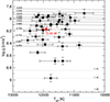 |
Fig. 1. Location of the sample of DAV stars considered in this work on the Teff − log g plane, depicted with black circles. Solid curves show the CO-core DA WD evolutionary tracks from Renedo et al. (2010), and dotted curves display the ultra-massive ONe-core DA WD evolutionary tracks from Camisassa et al. (2019), for different stellar masses. The location of the DAV star G 29−38 is emphasised with a red symbol. |
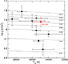 |
Fig. 2. Location of the sample of DBV stars considered in this work on the Teff − log g diagram, marked with black circles. Thin solid curves show the CO-core DB WD evolutionary tracks from Althaus et al. (2009) for different stellar masses. The location of the DBV star GD 358 is emphasised with a red symbol. |
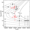 |
Fig. 3. Location of the sample of GW Vir variable stars considered in this work in the Teff − log g plane depicted with black circles. Thin solid curves show the CO-core PG 1159 evolutionary tracks from Miller Bertolami & Althaus (2006) for different stellar masses. The locations of the GW Vir stars PG 1159−035 (DOV type) and NGC 6904 (PNNV type) are marked with red symbols. |
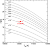 |
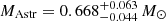
Fig. 4. Distance versus effective temperature curves corresponding to evolutionary sequences of DA WD models extracted from Renedo et al. (2010) with different stellar masses and for the apparent magnitude V of the DAV star G 29−38, whose location is indicated with a red circle with error bars. This star is characterised by Teff = 11 910 ± 162 K and dBJ = 17.51 ± 0.01 pc. The uncertainty in the distance is so small that it is contained within the symbol. From linear interpolation, the astrometric mass of G 29−38 is |
3.2. Seismological masses
We collected the seismological masses of pulsating WDs from asteroseismological models derived in the studies by Romero et al. (2012, 2013, 2017, 2019a), Córsico et al. (2019b), Romero et al. (2022, 2023), and Uzundag et al. (2023) for DAVs; Córsico et al. (2012), Bognár et al. (2014), Bell et al. (2019), Córsico et al. (2022b), and Córsico et al. (2022a) for DBVs; and Córsico et al. (2007, 2009), Kepler et al. (2014), Calcaferro et al. (2016), Córsico et al. (2021), Uzundag et al. (2021), Oliveira Rosa et al. (2022), and Calcaferro et al. (2024) for GW Vir stars. The seismological masses corresponding to DAV, DBV, and GW Vir stars derived from seismological models are provided in the third column of Tables B.1, B.2, and B.3. In the case of DBV and GW Vir stars, in many cases it has also been possible to estimate a seismological mass based on period spacing. These seismological masses are provided in the fourth column of Tables B.2 and B.3. We emphasise that the sample of DAV stars is comprised solely of objects with asteroseismological models characterised by a canonical (thick) H envelope. This explains why our sample of DAVs (Table A.1) is smaller than the total number of DAVs analysed seismologically to date.
3.3. Astrometric masses
We calculated astrometric masses using the following procedure. We built distance curves versus Teff by using Pogson’s law, which states that the distance of a star is given by log d = (V − MV + 5 − AV)/5, where V and MV represent the visual apparent and absolute magnitudes, respectively, and AV denotes the interstellar absorption in the V band. Using the bolometric correction (BC) from the WD grids of the Montreal Group4 (Bergeron et al. 1995; Holberg & Bergeron 2006; Bédard et al. 2020), the absolute visual magnitude was calculated as MV = MB − BC, where MB = MB⊙ − 2.5 log(L⋆/L⊙) and MB⊙ = 4.74 (Cox 2000). The function log(L⋆/L⊙) in terms of Teff for different values of M⋆ was obtained from the LPCODE WD evolutionary tracks provided by Renedo et al. (2010) (CO-core DA WDs) and Camisassa et al. (2019) (ONe-core ultra-massive DA WDs) for DAVs, Althaus et al. (2009) for DBVs, and Miller Bertolami & Althaus (2006) for GW Vir stars. Following Sowicka et al. (2023), the apparent visual magnitude V was evaluated based on the magnitudes G, GBP and GRPGaia using the expression
 (1)
(1)
extracted from Table 5.9 of Gaia DR3 documentation5. The uncertainties of G, GBP, and GRP produce errors in V. To estimate the uncertainties ΔG, ΔGBP and ΔGRP, we used the following expressions:
 (2)
(2)
where (S/N) is approximately equal to the parameter phot_g_mean_flux_over_error of the Gaia database6. We propagated the errors of G, GBP and GRP to V to obtain ΔV in the usual way (see the fourth column of Tables A.1, A.2, and A.3). We generated curves of d as a function of Teff for each stellar mass M⋆. We identified the target star based on its specified Teff and the distance extracted from Bailer-Jones et al. (2021) on the d versus Teff diagrams. By interpolating between these curves, we estimated the astrometric mass, MAstr. Each star has its own set of d versus Teff curves, as these curves depend on the star’s magnitude V. The resulting astrometric masses are provided in the fifth column of Table B.1 for DAVs, and the sixth column of Tables B.2 and B.3 for DBV and GW Vir stars.
In Fig. 4, we present a Teff − d diagram illustrating the case of the DAV star G 29−38, while Fig. 5 shows the DBV star GD 358. Furthermore, Figs. 6 and 7 highlight the GW Vir stars PG 1159−035 (DOV type) and NGC 6905 (PNNV type), respectively. For DAVs and DBVs, which are typically in close proximity to the Sun, the uncertainties in the distances provided by Bailer-Jones et al. (2021) are minimal, resulting in error bars that are contained within the symbols in Figs. 4 and 5. Consequently, the astrometric mass of these stars is primarily affected by uncertainties in Teff. In contrast, GW Vir stars are much more distant, leading to more significant uncertainties in their distances. This is evident in Figs. 6 and 7. For these stars, the uncertainties in the astrometric masses arise from both Teff errors and dBJ. Despite these challenges, the uncertainties in astrometric masses of GW Vir stars are generally comparable to those of seismological masses, and both are notably smaller than the uncertainties associated with spectroscopic masses (refer to Table B.3 and Sect. 4.3 for further details).
 |
Fig. 5. Distance versus effective temperature curves corresponding to evolutionary sequences of DB WD models extracted from Althaus et al. (2009) with different stellar masses and the apparent magnitude V of the DBV star GD 358 (red circle with error bars), characterised by Teff = 24 937 ± 1018 K and dBJ = 42.99 ± 0.05 pc. The uncertainty in the distance is so small that it is contained within the symbol. From linear interpolation, the astrometric mass of GD 358 is |
 |
Fig. 6. Distance versus effective temperature curves corresponding to evolutionary sequences of PG 1159 models extracted from Miller Bertolami & Althaus (2006) with different stellar masses and the apparent magnitude V corresponding to the GW Vir star (DOV-type) PG 1159−035. The location of this star is marked with a red circle with error bars. The star is characterised by Teff = 140 000 ± 5000 K and |

 |
Fig. 7. Distance versus effective temperature curves corresponding to evolutionary sequences of PG1159 models extracted from Miller Bertolami & Althaus (2006) with different stellar masses and the apparent magnitude V corresponding to the GW Vir star (PNNV-type) NGC 6905 (red circle with error bars), characterised by Teff = 141 000 ± 10 000 K and dBJ = 2700 ± 200 pc. From linear interpolation, the astrometric mass of NGC 6905 is |
3.4. Photometric masses
In the photometric method (see, e.g., Bergeron et al. 1997, 2019), the spectral energy distribution of a star is compared with model atmospheres using synthetic photometry. Magnitudes are converted to fluxes and compared with model fluxes averaged over the same filter bandpasses. The effective temperature (Teff) and solid angle (π(R⋆/D)2) are considered free parameters, and the atmospheric composition is typically assumed to be pure H or He. If the star’s distance (D) is known, often from trigonometric parallax measurements, its radius (R⋆) can be directly obtained, allowing for the calculation of the star’s mass using WD mass-radius relationships (M⋆ − R⋆).
The combination of accurate parallaxes from Gaia and optical photometry (e.g. SDSS ugriz, Pan-STARRS grizy, or Gaia) has made the photometric method a robust tool for determining WD parameters (see, e.g., Bergeron et al. 2019; Genest-Beaulieu & Bergeron 2019a; Gentile Fusillo et al. 2019, 2021; Tremblay et al. 2019). Notably, Genest-Beaulieu & Bergeron (2019a,b) provide a thorough comparison of the spectroscopic and photometric parameters of a large sample of DA and DB WDs.
In this work, we adopted a straightforward approach to determine the photometric mass of the DAV and DBV stars in our sample. We employed the catalogue from Gentile Fusillo et al. (2021), where Teff, log g, and M⋆ for a large selection of WDs were derived using the photometric method based on Gaia astrometry and photometry. To obtain the stellar radius – a parameter not tabulated in their catalogue – we combined their parameters with the same mass-radius relationships from Bédard et al. (2020) that they employed, yielding a model-independent value. Next, we applied our LPCODE WD mass-radius relationships to compute the photometric mass (Mphot), ensuring consistency with the other mass estimates in this study. The results are listed in the last columns of Tables B.1 and B.2. Regarding our sample of GW Vir stars, to our very best knowledge, there are no photometric mass or radius determinations. We hope that future studies will provide these determinations to complete the picture. However, the issue in this case is that these stars are exceptionally hot, resulting in an energy distribution in the optical spectrum that adheres to the Rayleigh-Jeans approximation. Consequently, this distribution becomes largely insensitive to effective temperature, as illustrated, for example, in Figure 3 of Bédard et al. (2020). Therefore, it seems unlikely that photometric parameters will be obtainable for these stars, at least not through the use of optical photometry.
4. Analysis
In this section, we assess the consistency of spectroscopic, seismological, astrometric, and photometric (although only for DAVs and DBVs) masses through comparisons. We also examine seismological masses derived from period spacing for DBVs and GW Vir stars whenever feasible. To gauge the linear correlation between two sets of masses, we employ the Pearson coefficient r (see, for instance, Benesty et al. 2009). This coefficient ranges from −1 to +1, with 0 indicating that there is no linear association, and a strong correlation as r approaches 1 in absolute value. However, a high correlation does not necessarily imply a good agreement between masses, as r measures the strength of the relationship, not the agreement itself. For a more suitable assessment of the agreement, we turn to the Bland-Altman analysis (Altman & Bland 1983; Giavarina 2015). This involves plotting mass differences against their average values, helping to identify biases and outliers. The agreement limits are defined as ±1.96σ, where σ represents the standard deviation of the differences. In our analysis, we adopt a stricter criterion, using ±1σ to define agreement limits, enabling the identification of outlier WD stars with significantly different masses derived from various methods.
4.1. DAV stars
We compare MSpec and MSeis, MSeis and MAstr, MSpec and MAstr, MPhot and MAstr, MSeis and MPhot, and MSpec and MPhot for DAV stars in Figs. 8 to 13. Upon inspection of the figures, significant agreement is observed among the different sets of masses, particularly for masses below ∼0.75 M⊙, a trend that becomes apparent upon examination of the Pearson linear correlation coefficient. It is evident that in all cases this coefficient exceeds ∼ + 0.8, indicating a strong correlation. However, we are also interested in knowing how closely the sets of mass values agree, discovering whether there are global biases or not, and finding outlier stars whose masses should be re-evaluated in future analyses.
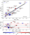 |
Fig. 8. Comparison of stellar masses for DAV stars. Upper panel: Dispersion diagram showing the comparison between the spectroscopic and the seismological masses for DAVs (see Table B.1). The blue dashed line indicates the 1:1 correspondence between the two sets of stellar masses. The labeled stars correspond to the cases where the mass estimates exhibit substantial discrepancies. The thick black line indicates the Pearson correlation fit. Lower panel: Bland-Altman diagram showing the mass difference in terms of the average mass for each object. The black short-dashed line corresponds to the mean difference, ⟨ΔM⋆⟩, whereas the two red dashed lines represent the limits of agreement, ⟨ΔM⋆⟩, considering the deviation of ±1σ. In both panels, the size of each symbol is proportional to the number of g-mode pulsation periods used to derive the seismological model (fourth column of Table B.1), and the colour palette indicates the apparent magnitude GaiaG (fifth column of Table A.1) of each star. |
We first start by comparing the stellar masses of DAVs obtained from spectroscopy and those corresponding to seismological models in a dispersion diagram, as shown in the upper panel of Fig. 8. In the figure, the blue dashed line represents the 1:1 line of correspondence between the two sets of stellar mass values. Stars whose mass estimates exhibit substantial discrepancies (i.e. deviate noticeably from the 1:1 line of correspondence) are labeled with their respective names. The Pearson coefficient, which measures the correlation between MSpec and MSeis in this case is r = +0.83, revealing a strong correlation. MSpec and MSeis show good agreement, which is somewhat anticipated, as seismological models are typically selected to satisfy the spectroscopic constraints of Teff and log g. This selection is made to mitigate the intrinsic degeneracy of solutions often encountered as a result of period-to-period fits (see, for instance, Romero et al. 2012, 2013). However, there are significant discrepancies for some stars more massive than ∼0.75 M⊙, as evidenced by their deviation from the 1:1 line of correspondence. The lower panel of the figure depicts the Bland-Altman diagram, where the mass differences, ΔM⋆ = MSeis − MSpec, are plotted against the mean mass value, ⟨M⋆⟩=(MSeis + MSpec)/2, for each star. The mean difference is ⟨ΔM⋆⟩ = 0.023, indicating a small positive bias represented by the gap between the x axis (corresponding to zero differences, marked by the dotted line) and the short-dashed line parallel to the x axis at 0.023 units. This suggests that on average, the seismological masses are somewhat higher than the spectroscopic ones. The limits of agreement, defined as the ±1σ departure from the mean difference, are displayed with red dashed lines at ⟨ΔM⋆⟩±0.089 M⊙. From this diagram, it is clear that there are outlier stars for which the mass difference is beyond the agreement limits, in accordance with what the dispersion diagram (upper panel) indicates. In these diagrams, the size of the symbols is directly proportional to the number of periods used to obtain the seismological models (fourth column of Table B.1), while the colour of each symbol is related to the brightness of the star (the apparent Gaia magnitude G in the bottom palette of colours). Clearly, most outlier stars are dim (high G value). One exception is BPM 37093, which is bright but nonetheless exhibits a large mass discrepancy. Furthermore, there is no clear indication that the number of periods is crucial for the star to have discrepant spectroscopic and seismological masses.
The comparison between seismological and astrometric masses (upper panel of Fig. 9) closely resembles the situation analysed above for spectroscopic and seismological masses (Fig. 8). It is evident that there is strong agreement between MSeis and MAstr, particularly for M⋆ ≲ 0.75 M⊙. However, discrepancies become more apparent for larger masses, with data points deviating further from the 1:1 identity line. The Pearson coefficient for this comparison is r = +0.86, indicating a robust correlation. In the Bland-Altman diagram (lower panel of Fig. 9), we observe a small negative mean mass difference of ⟨ΔM⋆⟩=⟨MAstr − MSeis⟩= − 0.005 M⊙, suggesting a slight negative bias between MSeis and MAstr masses (with MSeis tending to be slightly larger than MAstr on average). The limits of agreement, ⟨ΔM⋆⟩±0.083 M⊙, are very similar to those observed in the comparison between spectroscopic and seismological masses (Fig. 8). Once again, BPM 37093 stands out among outliers, exhibiting a significant discrepancy between seismological and astrometric masses despite being a bright object.
When comparing spectroscopic masses with astrometric masses, a very strong correlation is observed (r = 0.92, upper panel of Fig. 10). In particular, we can see a very dense crowding of points close to the 1:1 correspondence line for objects with masses less than ∼0.75 M⊙, while there are several more massive objects that deviate from the line of identity, reflecting considerable discrepancies in the value of the stellar mass depending on the method used to derive it. In the corresponding Bland-Altman diagram (lower panel), a slight bias towards larger astrometric masses than spectroscopic ones is observed, with a positive mean difference of ⟨ΔM⋆⟩=⟨MAstr − MSpec⟩= + 0.017 M⊙. The limits of agreement, ⟨ΔM⋆⟩±0.057 M⊙, suggest that the mass differences are less scattered compared to the previous analyses. Notably, all outlier stars in this case are dim.
Upon analysing the relationship between photometric and astrometric masses shown in Fig. 11, we find a very strong correlation, as indicated by the r = +0.93 value in the upper panel. MPhot and MAstr show a significant agreement, in general, which is not surprising given that, although determined through very different procedures, the two methods employ photometry and astrometry from Gaia. The agreement between photometric and astrometric masses is particularly true for stars with M⋆ ≲ 0.75 M⊙, while for some more massive stars, a deviation from the 1:1 line of correspondence is found. The Bland-Altman diagram (lower panel) reveals a positive mean mass difference of ⟨ΔM⋆⟩=⟨MAstr − MPhot⟩= + 0.042 M⊙, indicating a noticeable bias where astrometric masses exceed photometric masses. The limits of agreement, ⟨ΔM⋆⟩±0.055 M⊙, similarly to the previous case, are also less scattered than the first two cases (MSpec vs. MSeis and MSeis vs. MAstr). We also note that all the outlier stars in this case are dim.
In assessing the comparison between seismological and photometric masses, we find a similar dispersion diagram (upper panel in Fig. 12) as the one shown in the comparison between astrometric and seismological masses. In this case, r = +0.88, indicating again a strong correlation. It is clear that there is close agreement between the seismological and photometric masses, although some discrepancies are found, particularly for stars between, roughly, 0.7 and 1 M⊙. In the Bland-Altman diagram (lower panel in Fig. 12), there is a negative mean mass difference of ⟨ΔM⋆⟩=⟨MPhot − MSeis⟩= − 0.055 M⊙, indicating that photometric masses are, on average, larger than seismological masses. The limits of agreement, ⟨ΔM⋆⟩±0.083 M⊙ are also very similar to those found in the comparison between astrometric and seismological masses. In this case, as before, we once again find BPM 37093 as an outlier star.
Finally, when comparing spectroscopic and photometric masses, illustrated in Fig. 13, we observe a strong correlation as reflected by the r = +0.90 value shown in the upper panel. The Bland-Altman diagram (lower panel) indicates that there is a negative mean mass difference of ⟨ΔM⋆⟩=⟨MPhot − MSpec⟩= − 0.031 M⊙, implying that photometric masses are generally lower than spectroscopic masses. In this case, the limits of agreement are ⟨ΔM⋆⟩±0.063 M⊙, and it is clear that all outlier stars are dim.
In summary, the masses of DAV stars derived from the four methods considered generally show good agreement, particularly for masses below approximately 0.75 M⊙. However, there are notable discrepancies for certain DAV stars. Table B.4 lists the objects classified as outliers, where there are discrepancies between the mass values derived from different methods. An outlier is identified when ⟨M⋆⟩−σ ≥ ΔM⋆ ≥ ⟨M⋆⟩+σ. For outlier DAV stars BPM 37093, GALEX J1650+3010, GALEX J2208+0654, GALEX J0048+1521, SDSS J0843+0431, and EC 23487−2424, we observe MSeis > MAstr ≳ MSpec. This suggests that spectroscopic masses for these stars might be slightly underestimated, while seismological masses could be overestimated and require reassessment. Regarding BPM 37093, we note that the mass of this star would vary slightly if we were to use CO-core WD models. However, the seismological analysis of this star was performed using ONe core WD models (Córsico et al. 2019b). Therefore, for consistency, we used ONe-core WD evolutionary tracks in this paper to derive both spectroscopic and astrometric masses. It is interesting to note that the photometric mass of this star is very similar to the spectroscopic mass. Conversely, for SDSS J2159+1322 and GALEX J1257+0124, we find MSpec > MPhot ≳ MSeis ≳ MAstr, which indicates the potential overestimation of spectroscopic masses. TIC 167486543 and GALEX J1612+0830 exhibit MAstr > MSpec > MSeis, suggesting that both seismological and spectroscopic masses might be underestimated. Similarly, for the pair 2QZ J1323+0103 and KIC 11911480, we observe MAstr > MSeis ≳ MSpec, indicating the potential underestimation of both seismological and spectroscopic masses. The case of Ross 808 shows MSeis > MAstr ≃ MSpec ≃ MPhot, suggesting a possible overestimation of the seismological mass. Finally, for SDSS J1641+3521, we find MSpec > MSeis = MAstr > MPhot, indicating a potential overestimation of spectroscopic mass, necessitating a review of Teff and log g, and a potential underestimation of photometric mass.
4.2. DBV stars
We present comparisons between MSpec and MSeis, MSpec and MSeis(ΔΠ), MSeis and MAstr, MSpec and MAstr, MSpec and MPhot, MPhot and MAstr, MSeis and MPhot, and MPhot and MSeis(ΔΠ) for DBVs in Figs. 14 to 21. MSeis(ΔΠ) represents the seismological stellar mass derived on the basis of uniform period spacing. Among these figures, we observe two different levels of correlation. Five out of eight (Figures 14 to 18, displaying MSpec and MSeis, MSpec and MSeis(ΔΠ), MSeis and MAstr, MSpec and MAstr, and MSpec and MPhot) indicate a moderate linear correlation, with Pearson coefficients that do not exceed ∼ + 0.66, while the remaining three (Figures 19 to 21, showing MPhot and MAstr, MSeis and MPhot, and MPhot and MSeis(ΔΠ)) exhibit a stronger correlation, with Pearson coefficients that range from +0.77 to +0.92. Notably, of the four figures that involve comparisons with photometric masses, three of them are the ones showing a higher degree of correlation. This suggests a potential trend where comparisons involving photometric masses tend to exhibit a stronger correlation.
We first turn our attention to the cases with moderate correlation (Figures 14 to 18). The Bland-Pearson diagrams reveal significant biases among the methods of stellar mass derivation, indicating poor agreement among the various mass sets. Identifying outlier stars based on agreement limits becomes a challenge. In cases where there is a notable bias between the two mass sets, characterised by a mean difference considerably different from zero, a star may fall within admissibility limits because its distance from the mean difference, ⟨ΔM⋆⟩, is within ±σ. However, it could still be located far from the 1:1 correspondence line, indicating significant mass discrepancies. Conversely, an object may appear close to the 1:1 correspondence line, suggesting good mass agreement, but fall outside admissibility limits in the Bland-Altman diagram, leading to erroneous outlier classification.
Notably, a consistent trend is observed in most comparisons: spectroscopic masses are systematically smaller than seismological and astrometric masses. For example, in Fig. 14, where seismological masses are compared with spectroscopic masses, seven out of nine DBV stars exhibit spectroscopic masses smaller than seismological masses. This trend is evident in the mean mass difference of ⟨ΔM⋆⟩ = 0.034 M⊙, indicating a notable bias towards seismological masses being greater than spectroscopic masses. It is important to note that the limits of agreement, ⟨ΔM⋆⟩±0.079 M⊙, prove to be inappropriate to identify outliers. In fact, KUV 05134+2605, KIC 8626021, and PG 1351+489 clearly stand out as outliers, positioned significantly away from the 1:1 correspondence line, despite falling at the upper limit of agreement. TIC 257459955 is also evidently an outlier, despite falling within the agreement limits.
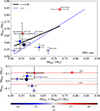 |
Fig. 14. Comparison of stellar masses for DBV stars. Upper panel: Dispersion diagram displaying the comparison between the spectroscopic and asteroseismological masses for DBVs (see Table B.2). All the stars are identified by their names. Bottom panel: Corresponding Bland-Pearson diagram. The meaning of the different lines in both panels is the same as in Fig. 8. |
The discrepancy between different sets of masses becomes more apparent when comparing spectroscopic masses with seismological masses derived from period spacing (Fig. 15). In this comparison, seven out of nine stars exhibit spectroscopic masses smaller than their seismological counterparts. It is important to note that for two stars (PG 1351+489 and EC 20058−5234), the seismological mass is defined within a range of values (see Table B.2), where we have taken the average value of both extremes as the seismological mass. The bias towards larger seismological masses compared to spectroscopic ones is more pronounced here, with an average mass difference of ⟨ΔM⋆⟩ = 0.085 M⊙. Unfortunately, the Bland-Altman diagram does not effectively identify outliers. For instance, despite KUV 05134+2605 and KIC 8626021 being outliers according to the scatter plot, they fall well within the limits of agreement in the Bland-Altman diagram.
In the comparison between seismological and astrometric masses (Fig. 16), it is clear that astrometric masses generally exceed seismological masses, with an average mass difference of ⟨ΔM⋆⟩ = 0.045 M⊙. Furthermore, when comparing spectroscopic masses with astrometric masses (Fig. 17), it is noteworthy that all spectroscopic masses are below the astrometric masses. Here, the average mass difference amounts to ⟨ΔM⋆⟩ = 0.079 M⊙. In fact, spectroscopic masses are approximately 14% smaller than astrometric masses on average. Validating this trend would require analysing a broader sample of DB WD stars, a task planned for a future paper.
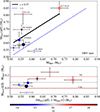 |
Fig. 15. Similar to Fig. 14, this figure illustrates the comparison between spectroscopic and seismological masses, with the seismological mass derived from the period spacing (ΔΠ). It is worth noting that only seven out of the total nine DBV stars analysed have an estimate of seismological mass from the period spacing (see Table B.2). |
The observed trend of spectroscopic masses being systematically smaller than the other mass estimates does not hold, however, when comparing them to photometric masses, as shown in Fig. 18. Indeed, we find a slight bias towards larger photometric masses, reflected in the mean mass difference ⟨ΔM⋆⟩ = 0.013 M⊙. The lower panel reveals that the limits of agreement, ⟨ΔM⋆⟩±0.065 M⊙, are once again inadequate for identifying outliers. This is evident from L7−44 and EC 20058−5234, which, despite being clear outliers in the upper panel, fall within or almost exactly on the limits of agreement in the lower panel.
Now we focus on the cases exhibiting strong correlations, specifically between MPhot and MAstr, MPhot and MSeis(ΔΠ), and MSeis and MPhot. In the first case, where we compare photometric and astrometric masses, as illustrated in Fig. 19, the Pearson coefficient is high, r = +0.92. The upper panel clearly shows that all astrometric masses surpass the photometric ones, similar to what is found in the comparison between spectroscopic and astrometric masses. Here, the mean mass difference is ⟨ΔM⋆⟩ = 0.045 M⊙, and we find that astrometric masses are approximately 11% greater than their photometric counterparts. Confirming this trend between astrometric and photometric masses will necessitate further analysis with a larger sample of DB WDs, as already mentioned and planned for future work.
When comparing seismological and photometric masses, a strong correlation is evident, with a Pearson coefficient of r = +0.80, as shown in the upper panel of Fig. 20. This is particularly true for stars with masses ≲0.6 M⊙. In the lower panel, the mean mass difference of ⟨ΔM⋆⟩= − 0.021 M⊙ indicates that seismological masses slightly exceed photometric ones. Lastly, Fig. 21 presents the comparison between MPhot and MSeis(ΔΠ). The correlation in this case is r = +0.77, slightly lower than in the previous case. However, it remains evident that objects with masses ≲0.6 M⊙ are close to the 1:1 correspondence line. The mean mass difference of ⟨ΔM⋆⟩ = 0.031 M⊙ indicates a tendency for seismological masses derived from the period spacing to be slightly larger than photometric ones.
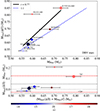 |
Fig. 21. Similar to Fig. 15 but for the comparison between photometric and seismological masses derived from the period spacing. |
In the following, we delve into describing the significant discrepancies observed in some of the DBV stars. We provide below a detailed analysis of cases where notable disagreements arise.
-
KUV 05134+2605: With an extensive dataset of 16 detected periods, but not being very bright (G = 16.749), this star exhibits the trend MSeis ≃ MSeis(ΔΠ) > MAstr ≳ MPhot ≃ MSpec. The masses derived from asteroseismology (MSeis, MSeis(ΔΠ)) appear notably high among the other estimates, in clear contrast to the low value of the spectroscopic mass (MSpec). Given the close agreement between MPhot, MSpec, and MAstr, our results might suggest that the higher masses obtained from asteroseismology warrant a re-evaluation.
-
KIC 8626021: Here, we observe MAstr > MSeis(ΔΠ)≃MPhot ≃ MSeis > MSpec. This star, with a faint brightness (G = 18.500) and a limited number of periods (5), exhibits a notably small spectroscopic mass, highlighting the need for a thorough revision of the spectroscopic parameters (Teff and log g).
-
PG 1351+489: In this case, we find MSeis(ΔΠ) > MSeis ≃ MAstr > MPhot > MSpec. The seismological mass derived from the period spacing appears to be notably high (0.740 ≲ M⋆/M⊙ ≲ 0.870). In contrast, the spectroscopic mass is markedly low, indicating a need for refinement to determine Teff and log g.
-
WD J1527−4502: For this star, we get MAstr ≳ MSpec > MPhot > MSeis, suggesting that the spectroscopic mass is well determined, but the seismological mass is low in excess. The photometric mass is also lower compared to MAstr and MSpec, but to a lesser extent than the seismological mass. For this star, there is no assessment of the seismological mass based on the period spacing. Our results suggest a review of the seismological mass of WD J1527−4502.
It is worth highlighting that, beyond these four troublesome stars, the remaining DBV stars in the small sample show varying degrees of inconsistency in their mass values depending on the method used. Below, we describe each one of these cases:
-
EC 20058−5234: In this case, we observe MSeis > MSpec ≃ MAstr > MPhot ≃ MSeis(ΔΠ). This suggests the reliability of the spectroscopic mass, which aligns with the astrometric mass. However, the seismological mass derived from individual periods appears to be overstated. Interestingly, the photometric mass aligns well with the seismological mass based on period spacing, although both of these are lower compared with the spectroscopic and astrometric values. Consequently, a reassessment of the seismological determinations of EC20058−5234’s mass seems warranted.
-
TIC 257459955: In this case, MAstr ≃ MSeis(ΔΠ)≃MSeis ≃ MPhot > MSpec, indicating a notably low spectroscopic mass. Therefore, a reevaluation of the parameters Teff and log g, utilised to derive the spectroscopic mass, appears to be necessary.
-
EC 04207−4748: Here, MAstr > MPhot ≃ MSeis ≃ MSeis(ΔΠ) > MSpec. This suggests an underestimation of the spectroscopic mass, implying a need for a reassessment of the spectroscopic parameters for this star.
-
L 7−44: Here, we find MAstr ≳ MSpec > MPhot > MSeis, suggesting an underestimation of the seismological mass, which warrants a re-assessment.
-
GD 358: As the prototype of DBV stars (also known as V777 Her stars), we observe MAstr ≳ MSeis ≃ MSeis(ΔΠ)≃MPhot > MSpec. These findings imply a possible underestimation of the spectroscopic mass of GD 358. Therefore, it is advisable to reevaluate the spectroscopic parameters (Teff and log g) utilised to calculate MSpec.
We conclude our analysis of the DBV stars by highlighting a trend that is consistent across most cases: the spectroscopic mass values appear to be systematically underestimated. This observation raises the possibility of encountering challenges in precisely determining Teff and log g through spectroscopic methods for DBV stars (see Sect. 5). Similar to DAVs, we do not observe a direct correlation between the reliability of seismological mass determination and either the star’s brightness or the number of periods used in determining the seismological mass.
4.3. GW Vir stars
In this section, we present comparisons between MSpec and MSeis, MSpec and MSeis(ΔΠ), MSeis and MAstr, and MSpec and MAstr for GW Vir stars in Figures 22, 23, 24, and 25, respectively. As we established before, for this class of pulsating stars we do not have available photometric radii or masses, which prevents us from considering comparisons with MPhot.
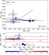 |
Fig. 22. Comparison of stellar masses for GW Vir stars. Upper panel: dispersion diagram showing the comparison between the spectroscopic and asteroseismological masses for GW Vir stars (refer to Table B.3). Stars with mass estimates that significantly disagree are annotated with their names. Bottom panel: corresponding Bland-Pearson diagram. The meaning of the different lines in both panels is the same as in Fig. 8. |
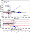 |
Fig. 23. Similar to Fig. 22, this figure presents the comparison between spectroscopic and seismological masses, where the seismological masses are derived from the period spacing (ΔΠ). |
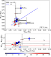 |
Fig. 24. Similar to Fig. 22, this figure displays the comparison between seismological and astrometric masses. |
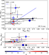 |
Fig. 25. In analogy to Fig. 22, this figure illustrates the comparison between spectroscopic and astrometric masses. |
Let us begin by examining the comparison between the spectroscopic and seismological masses of GW Vir stars. From the upper panel of Fig. 22, it is evident that there is generally good agreement between the two sets of masses, as indicated by their proximity to the 1:1 identity line. However, certain stars exhibit significant discrepancies. For example, the seismological masses are significantly larger (by approximately 20%) than the spectroscopic masses for NGC 2371 and HS 2324+3944, while for others, such as RX J2117+3412 and NGC 246, the spectroscopic mass exceeds the seismological mass by approximately 30%. In this case, the Pearson coefficient is small and negative (r = −0.15), suggesting a weak and meaningless anticorrelation between the two sets of masses. Pearson’s linear correlation analysis loses meaning in this case. On the other hand, the Bland-Altman diagram (bottom panel) illustrates that most stars cluster near the mean value of the mass differences, which is very small (⟨ΔM⋆⟩ = 0.013 M⊙). This indicates a negligible bias between the two mass sets, with only four outlier stars deviating beyond the limits of agreement (⟨ΔM⋆⟩±0.087 M⊙). These outliers include RX J2117+2117 and NGC 246 (where MSpec > MSeis), and HS 2324+3944 and NGC 2371 (where MSpec < MSeis).
Something completely analogous happens when comparing the spectroscopic masses with the seismological masses derived from the period spacing (Fig. 23). Once again, significant disparities are evident between the spectroscopic and seismological masses of the same stars NGC 2371, HS 2324+3944, RX J2117+3412, and NGC 246. In this case, the Pearson coefficient is r = −0.25, indicating a weak anticorrelation between MSeis(ΔΠ) and MSpec. A feature worth highlighting is that the uncertainties of the spectroscopic masses are by far greater than the seismological ones. This is due to the enormous uncertainties in the spectroscopic parameters of GW Vir stars, in particular in surface gravity (see Table A.3). This is a clear symptom of the difficulty in modelling the atmospheres of these extremely hot stars (see Sect. 5).
The comparison between seismological and astrometric masses of GW Vir stars is depicted in Fig. 24. Here, the Pearson coefficient is extremely small (r = −0.01), indicating a negligible correlation between MSeis and MAstr. The Bland-Altman diagram reveals an almost negligible bias between the seismological and astrometric masses, with an average difference of ⟨ΔM⋆⟩ = 0.0004 M⊙. This suggests a very close agreement between both methods for deriving the masses of GW Vir stars on average. Moreover, the diagram highlights the presence of some outliers, whose mass differences exceed the agreement limits. These limits, set at ⟨ΔM⋆⟩±0.085 M⊙, are surpassed by SDSS J0754+0852 and NGC 1501, where MAstr > MSeis, as well as HS 2324+3944 and NGC 3271, which exhibit MAstr < MSeis.
Finally, in Fig. 25, we explore the compatibility between spectroscopic and astrometric masses. Once again, the large size of the error bars associated with the spectroscopic masses is noteworthy, indicating the substantial uncertainties in deriving log g through spectroscopy. In this case, the Pearson coefficient is r = +0.06, indicating again a negligible linear correlation. The average of the mass differences is in this case ⟨ΔM⋆⟩ = 0.013 M⊙, and the agreement limits are ⟨ΔM⋆⟩±0.101 M⊙. Also notable in this case is the strong discrepancy between the spectroscopic mass and the astrometric mass in several objects, such as NGC 1501, SDSS J0754+0852, NGC 246, and RX J2117+3412.
In summary, there is consensus among the sets of stellar masses for some GW Vir stars derived using three (or four) different methods, although there are outliers where mass determinations by various methods display significant discrepancies. In the following, we delve into each of these cases.
-
HS 2324+3944: For this star, we find MSeis(ΔΠ) > MSeis > MAstr ≃ MSpec. This suggests that the seismological masses are overestimated, particularly the one based on period spacing, while the spectroscopic mass, which closely matches the astrometric mass, appears to be well-determined.
-
NGC 2371: The situation for this star is analogous to the case of HS 2324+3944, where the different estimates of the stellar mass verify the inequalities MSeis(ΔΠ) > MSeis > MAstr ≳ MSpec. So, again, we conclude that the seismological masses are overestimated.
-
RX J2117+3412: This star presents a notable scenario where MSpec > MAstr ≳ MSeis(ΔΠ)≳MAstr. Unlike previous cases, the spectroscopic mass of RX J2117+3412 appears to be overstated, suggesting a potential need to re-assess the parameters Teff and log g derived from spectroscopic analysis.
-
NGC 246: This is a twin case to the RX J2117+3412 case (MSpec > MAstr ≳ MSeis(ΔΠ)≳MAstr). We suggest that the spectroscopic parameters of NGC 246, and thus the evaluation of its spectroscopic mass, need to be revised. Both NGC 246 and RX J2117+3412 exhibit P Cygni line profiles in the ultraviolet wavelength region that allowed their mass-loss rates to be measured (Koesterke & Werner 1998). It would be worthwhile to repeat the analysis of their optical spectra using expanding model atmospheres instead of hydrostatic ones that were employed to determine the spectroscopic parameters.
-
NGC 1501: In this case, we find MAstr > MSeis ≃ MSeis(ΔΠ)≳MSpec. In this way, we conclude that the seismological and spectroscopic masses of NGC 1501 are quite low, and then Teff and log g need to be revised. We remark that it is not trivial to determine effective temperature and surface gravity of [WR] stars, because they have extended atmospheres. One has to define precisely the stellar radius, as this affects the values of temperature and gravity. In addition, using such atmosphere models as boundary conditions for evolution calculations could be significant for the location of the tracks in the Hertzsprung-Russell Diagram (HRD).
-
SDSS J0754+0852: For this star, we have MAstr > MSeis > MSpec, the situation being completely analogous to the case of NGC 1501: the seismological and spectroscopic masses are quite small. We suggest revising the seismological and spectroscopic masses and reevaluating the spectroscopic parameters of SDSS J0754+0852. We note, however, that the astrometric mass error is the largest of all GW Vir stars because it is very faint.
5. Discussion
The results of the previous section point to several cases of important discrepancies between the masses derived through different methods for the three classes of pulsating WDs examined. In particular, we found situations in which the spectroscopic mass is in significant disagreement with the other mass determinations. In other cases, it is the seismological mass that is dissonant. In this section, we discuss some of the possible reasons that could explain, at least in part, the discrepancies found.
When considering stars with spectroscopic masses that disagree with other determinations, it becomes apparent that the uncertainties in determining MSpec for WDs are closely related to uncertainties in determining the effective temperature and surface gravity. The accuracy of spectroscopic determinations depends heavily on the input physics incorporated into atmosphere models, particularly with respect to the reliability of modelled line profiles, especially in ultraviolet and optical spectra. Factors such as line broadening and convective energy transport significantly influence the shape and intensity of spectral lines (Saumon et al. 2022).
Various systematic effects impact the assessment of Teff and log g for WDs, particularly pulsating WDs. Fuchs (2017) spectroscopically observed 122 DA WDs that either pulsate or are close to the DAV instability strip and estimated Teff and log g for each WD based on Balmer line profile shapes. They conducted a meticulous study of several systematics involved in data reduction and spectral fitting procedures, including extinction correction, flux calibration, and signal-to-noise ratios of the spectra, which can affect the final atmospheric parameters Teff and log g. They concluded that neglecting these systematic effects could introduce errors in atmospheric parameter determinations, potentially affecting the determination of spectroscopic masses for DAVs.
Similarly to DAVs, the determination of Teff and log g for DBVs is subject to uncertainties arising from various sources, such as the input physics of atmosphere models, signal-to-noise ratio of spectra, use of different data sets, and accuracy of flux calibrations (see, e.g., Izquierdo et al. 2023). Specifically, in the case of the model atmosphere fit, precise values of Teff are difficult to obtain within the range of ∼21 000 − 31 000 K. Here, a plateau in the strength of the HeI absorption lines results in hot and cold solutions for Teff due to the insensitivity of these lines to changes in temperature (Bergeron et al. 2011). This overlap with the DBV instability strip complicates their characterisation (Vanderbosch et al. 2022).
Notably, the photometric method provides an alternative value of the effective temperature as part of the fitting process itself, as previously mentioned. In fact, the photometric technique in DA WDs appears to be more accurate than the spectroscopic technique for the Teff determination, as Genest-Beaulieu & Bergeron (2019a) show. However, these authors also state that both techniques have a similar accuracy at determining the stellar masses of DA WDs. For DB WDs, Genest-Beaulieu & Bergeron (2019b) report that both techniques yield the effective temperature with comparable accuracy, but the photometric technique is a superior option for the estimation of WD masses. Overall, this technique is generally more advantageous because broadband fluxes are significantly less affected by the complexities of the atomic physics and the equation-of-state compared to line profiles. Nonetheless, its accuracy relies on the photometric calibration (Serenelli et al. 2021).
Finally, both Teff and log g in GW Vir stars exhibit considerable uncertainties. As shown in Table A.3, Teff uncertainties are generally manageable, typically within 10%. When UV spectra or high-resolution and high S/N ratio optical spectra are available, the error can decrease to approximately 5%. In particular, the presence of metal lines, often found in UV or optical spectra, serves as a valuable tool to constrain Teff (Werner & Rauch 2014). However, log g uncertainties pose a significant challenge. Although errors for DAs and DBs typically hover around 0.05 dex, they can escalate to approximately 0.5 dex for GW Vir stars, with only a few exceptions as low as 0.3 or 0.2 dex, as detailed in Table A.3. The main problem is that the primary gravity indicator, the wings of the HeII line, exhibits weak sensitivity to variations of log g, which directly affects the determination of gravity. Existent uncertainties in line-broadening theory also affect this determination. Moreover, the normalisation of optical spectra introduces systematic errors due to challenges in determining the true continuum, particularly given the width of the HeII (and CIV) lines. It is important to note that in the determinations of log g of GW Vir stars from the Tübingen group (see, e.g., Werner & Herwig 2006) not only are internal errors taken into account, coming from spectrum fits, but systematic errors are also accounted for, an aspect that may explain the relatively higher values of the uncertainty of log g compared to the other classes of pulsating WD stars studied in this work.
When considering stars with notably discrepant seismological masses, it becomes apparent that revisions may be necessary in the derivation of seismological models. Our analysis suggests that neither the number of pulsation periods nor the apparent brightness of pulsating WDs can be directly linked to the reliability of MSeis determination. Specifically, having numerous periods available for asteroseismology does not guarantee the identification of a single and robust seismological solution. Instead, it is the distribution of these periods, particularly in terms of radial order, that significantly influences solution uniqueness or degeneracy. This issue has been exemplified in the case of DAVs by Giammichele et al. (2017), who demonstrated that even with a limited number of modes, precise determination of core chemical stratification can be achieved due to the considerable sensitivity of certain confined modes to partial mode trapping effects. Moreover, they highlighted that the ability to unravel the core structure and obtain a unique seismological model depends on the information content of available seismological data in terms of the weight functions7 of the observed g-modes. In some cases, the isolation of a unique and well-defined seismological solution can prove challenging, leaving the problem degenerate. An additional factor contributing to potential errors in seismological model derivation is the inherent symmetry observed in high-overtone stellar pulsations as they probe both the core and envelope of pulsating WDs (Montgomery et al. 2003). This symmetry has the potential to introduce ambiguity in the derived internal structure locations, as well as in the seismological models themselves. Finally, the choice of the asteroseismological approach and the criteria for selecting seismological models, when faced with a range of potential solutions, may influence the determination of the seismological mass, eventually leading to discrepancies compared to masses derived from other methods. In other cases, for stars with a limited number of periods, seismological analyses may resort to models constrained by external parameters such as spectroscopic Teff and log g. In these instances, we observe an obvious close alignment between the seismological and spectroscopic masses.
We close this section by pointing out that there could be possible systematic uncertainties in the WD evolutionary tracks that would affect the determination of the four types of mass determination, including the astrometric mass because this method uses the luminosity versus the effective temperature extracted from the evolutionary tracks, as well as the photometric mass, because of the use of the mass-radius relationships. It is important for future studies of this nature to employ alternative sets of WD evolutionary tracks, distinct from those used in this paper generated using the LPCODE evolutionary code. Concerning our results regarding the masses of the DAVs, the observed dispersion across various methods becomes particularly notable for masses exceeding approximately 0.75 M⊙ (Figs. 8, 9, 10, and 11). Assessing whether this phenomenon reflects genuine discrepancies rooted in unexplored aspects of WD structure and evolution requires the examination of a substantially larger sample of objects. Investigating such a broader dataset will be the primary focus of future research.
6. Conclusions
In this paper, we conduct a comparative analysis to determine the level of agreement between various methodologies used in determining the stellar mass of isolated pulsating WDs. We compute the stellar mass for a sample of selected DAV, DBV, and GW Vir stars using four distinct approaches: spectroscopy, asteroseismology, astrometry, and photometry (although the latter was only applied for DAVs and DBVs). Specifically, we used the spectroscopic measurements of Teff and log g, along with WD evolutionary tracks, to estimate spectroscopic masses. Seismological mass values were sourced from the existing literature. Additionally, we derived astrometric masses using evolutionary tracks, spectroscopic effective temperatures, apparent magnitudes, and geometric distances obtained from Gaia parallaxes, as well as bolometric corrections from model atmospheres. We also utilised photometric masses and photometric effective temperatures from the literature, which have been determined using Gaia parallaxes and photometry combined with synthetic fluxes from model atmospheres. These values are then integrated with our evolutionary tracks to derive our own photometric masses. Our methodology involved employing identical evolutionary tracks and WD models in all methods. In particular, for assessing spectroscopic, astrometric, and photometric masses, we applied the same evolutionary tracks linked to sets of WD stellar models used in the asteroseismological analyses to derive seismological masses. This approach ensures coherence and reliability in comparing the four estimates of stellar mass.
The results of our analysis vary according to the category of pulsating WD considered. For DAVs, there is broad consensus among the four methods for stars with masses up to around ∼0.75 M⊙, but significant inconsistencies emerge for more massive DAVs (Figs. 8, 9, 10, and 11). Assessing whether this phenomenon reflects genuine discrepancies rooted in unexplored aspects of WD structure and evolution requires the examination of a substantially larger sample of objects. Investigating such a broader dataset will be the primary focus of future research. Regarding the examined DBVs, almost all objects in the sample exhibit astrometric masses that surpass their seismological, spectroscopic, and photometric counterparts (Figs. 16, 17, and 19). Finally, for GW Vir stars, while some display strong agreement among MSpec, MSeis, and MAstr, others reveal substantial disparities (Figs. 22, 23, 24 and 25). The dispersion of M⋆ values of the three classes of pulsating WDs considered in this paper, depending on the method used, suggests the need to re-assess the derivation of spectroscopic parameters (Teff and log g), as well as to revise the seismological models for some stars. Also, there is a need to continue improvements in the parallax measurements to exclude any possible astrometric error.
Future spectroscopic and photometric observations of pulsating WDs, particularly those deficient in H, are crucial for a more thorough comparison of these stars. We emphasise the importance of discovering pulsating WDs in eclipsing binaries, as this provides an opportunity to independently test seismological models. Ongoing and forthcoming large-scale spectroscopic surveys such as the Large Sky Area Multi-Object Fiber Spectroscopic Telescope (LAMOST; Cui et al. 2012), Sloan Digital Sky Survey V (SDSS-V; Kollmeier et al. 2017), WEAVE (Dalton et al. 2012), and 4MOST (de Jong et al. 2019) will play a significant role in confirming the spectroscopic classifications of pulsating WDs and expanding the sample size. Furthermore, ongoing and upcoming photometric observations from space missions such as the Transiting Exoplanet Survey Satellite (TESS; Ricker et al. 2015) and (PLATO; Rauer et al. 2014), respectively, as well as ground-based initiatives such as the Large Synoptic Survey Telescope (LSST; Ivezić et al. 2019) and BlackGEM (Bloemen et al. 2016), will offer valuable insights into the nature of variability among pulsating WDs and allow the discovery of more pulsation periods for better modelling.
We do not consider in this study the pulsating low-mass and extremely low-mass helium-core WDs (also known as ELMVs; see, e.g., Córsico et al. 2019a), that are also hydrogen-rich atmosphere WDs, the results of which will be presented in a separate work (Calcaferro et al., in prep.).
Weight functions pinpoint the internal regions of the star that influence the period of the mode, providing insight into its sensitivity to specific parts (Kawaler et al. 1985; Townsend & Kawaler 2023).
Acknowledgments
We would like to express our sincere gratitude to our referee, Prof. Pierre Bergeron, for his generous support and assistance, which significantly enhanced the scientific content of this paper. Part of this work was supported by AGENCIA through the Programa de Modernización Tecnológica BID 1728/OC-AR, and by the PIP 112-200801-00940 grant from CONICET. M. U. gratefully acknowledges funding from the Research Foundation Flanders (FWO) through a junior postdoctoral fellowship (grant agreement No. 1247624N). This research has used NASA Astrophysics Data System Bibliographic Services and the SIMBAD and VizieR databases, operated at CDS, Strasbourg, France.
References
- Althaus, L. G., & Córsico, A. H. 2022, A&A, 663, A167 [NASA ADS] [CrossRef] [EDP Sciences] [Google Scholar]
- Althaus, L. G., Panei, J. A., Miller Bertolami, M. M., et al. 2009, ApJ, 704, 1605 [Google Scholar]
- Althaus, L. G., Córsico, A. H., Isern, J., & García-Berro, E. 2010, A&ARv, 18, 471 [NASA ADS] [CrossRef] [Google Scholar]
- Altman, D. G., & Bland, J. M. 1983, Statistician, 32, 307 [CrossRef] [Google Scholar]
- Bailer-Jones, C. A. L., Rybizki, J., Fouesneau, M., Demleitner, M., & Andrae, R. 2021, AJ, 161, 147 [Google Scholar]
- Bédard, A., Bergeron, P., Brassard, P., & Fontaine, G. 2020, ApJ, 901, 93 [Google Scholar]
- Bedin, L. R., Salaris, M., Piotto, G., et al. 2009, ApJ, 697, 965 [NASA ADS] [CrossRef] [Google Scholar]
- Bedin, L. R., Salaris, M., Anderson, J., et al. 2015, MNRAS, 448, 1779 [NASA ADS] [CrossRef] [Google Scholar]
- Bell, K. J., Córsico, A. H., Bischoff-Kim, A., et al. 2019, A&A, 632, A42 [NASA ADS] [CrossRef] [EDP Sciences] [Google Scholar]
- Benesty, J., Chen, J., Huang, Y., & Cohen, I. 2009, Noise Reduction in Speech Processing (New York: Springer), 37 [Google Scholar]
- Bergeron, P., Saffer, R. A., & Liebert, J. 1992, ApJ, 394, 228 [NASA ADS] [CrossRef] [Google Scholar]
- Bergeron, P., Wesemael, F., & Beauchamp, A. 1995, PASP, 107, 1047 [Google Scholar]
- Bergeron, P., Ruiz, M. T., & Leggett, S. K. 1997, ApJS, 108, 339 [Google Scholar]
- Bergeron, P., Leggett, S. K., & Ruiz, M. T. 2001, ApJS, 133, 413 [Google Scholar]
- Bergeron, P., Wesemael, F., Dufour, P., et al. 2011, ApJ, 737, 28 [Google Scholar]
- Bergeron, P., Dufour, P., Fontaine, G., et al. 2019, ApJ, 876, 67 [NASA ADS] [CrossRef] [Google Scholar]
- Bloemen, S., Groot, P., Woudt, P., et al. 2016, SPIE Conf. Ser., 9906 [Google Scholar]
- Bognár, Z., Paparó, M., Córsico, A. H., Kepler, S. O., & Győrffy, Á. 2014, A&A, 570, A116 [NASA ADS] [CrossRef] [EDP Sciences] [Google Scholar]
- Bond, H. E., Gilliland, R. L., Schaefer, G. H., et al. 2015, ApJ, 813, 106 [Google Scholar]
- Bond, H. E., Bergeron, P., & Bédard, A. 2017a, ApJ, 848, 16 [NASA ADS] [CrossRef] [Google Scholar]
- Bond, H. E., Schaefer, G. H., Gilliland, R. L., et al. 2017b, ApJ, 840, 70 [Google Scholar]
- Caiazzo, I., Burdge, K. B., Fuller, J., et al. 2021, Nature, 595, 39 [CrossRef] [Google Scholar]
- Calcaferro, L. M., Córsico, A. H., & Althaus, L. G. 2016, A&A, 589, A40 [NASA ADS] [CrossRef] [EDP Sciences] [Google Scholar]
- Calcaferro, L. M., Sowicka, P., Uzundag, M., et al. 2024, A&A, 686, A140 [NASA ADS] [CrossRef] [EDP Sciences] [Google Scholar]
- Camisassa, M. E., Althaus, L. G., Córsico, A. H., et al. 2019, A&A, 625, A87 [NASA ADS] [CrossRef] [EDP Sciences] [Google Scholar]
- Campos, F., Kepler, S. O., Bonatto, C., & Ducati, J. R. 2013, MNRAS, 433, 243 [NASA ADS] [CrossRef] [Google Scholar]
- Campos, F., Bergeron, P., Romero, A. D., et al. 2016, MNRAS, 456, 3729 [NASA ADS] [CrossRef] [Google Scholar]
- Catalán, S., Isern, J., García-Berro, E., & Ribas, I. 2008, MNRAS, 387, 1693 [Google Scholar]
- Chambers, K. C., Magnier, E. A., Metcalfe, N., et al. 2016, ArXiv e-prints [arXiv:1612.05560] [Google Scholar]
- Ciardullo, R., & Bond, H. E. 1996, AJ, 111, 2332 [CrossRef] [Google Scholar]
- Córsico, A. H. 2020, Front. Astron. Space Sci., 7, 47 [Google Scholar]
- Córsico, A. H. 2022, Boletin de la Asociacion Argentina de Astronomia La Plata Argentina, 63, 48 [Google Scholar]
- Córsico, A. H., & Althaus, L. G. 2006, A&A, 454, 863 [NASA ADS] [CrossRef] [EDP Sciences] [Google Scholar]
- Córsico, A. H., Miller Bertolami, M. M., Althaus, L. G., Vauclair, G., & Werner, K. 2007, A&A, 475, 619 [NASA ADS] [CrossRef] [EDP Sciences] [Google Scholar]
- Córsico, A. H., Althaus, L. G., Miller Bertolami, M. M., & García-Berro, E. 2009, A&A, 499, 257 [NASA ADS] [CrossRef] [EDP Sciences] [Google Scholar]
- Córsico, A. H., Althaus, L. G., Miller Bertolami, M. M., & Bischoff-Kim, A. 2012, A&A, 541, A42 [CrossRef] [EDP Sciences] [Google Scholar]
- Córsico, A. H., Althaus, L. G., Miller Bertolami, M. M., & Kepler, S. O. 2019a, A&ARv, 27, 7 [Google Scholar]
- Córsico, A. H., De Gerónimo, F. C., Camisassa, M. E., & Althaus, L. G. 2019b, A&A, 632, A119 [NASA ADS] [CrossRef] [EDP Sciences] [Google Scholar]
- Córsico, A. H., Uzundag, M., Kepler, S. O., et al. 2021, A&A, 645, A117 [EDP Sciences] [Google Scholar]
- Córsico, A. H., Uzundag, M., Kepler, S. O., et al. 2022a, A&A, 668, A161 [NASA ADS] [CrossRef] [EDP Sciences] [Google Scholar]
- Córsico, A. H., Uzundag, M., Kepler, S. O., et al. 2022b, A&A, 659, A30 [NASA ADS] [CrossRef] [EDP Sciences] [Google Scholar]
- Cox, A. N. 2000, Allen’s Astrophysical Quantities [Google Scholar]
- Cui, X.-Q., Zhao, Y.-H., Chu, Y.-Q., et al. 2012, Res. Astron. Astrophys., 12, 1197 [Google Scholar]
- Cukanovaite, E., Tremblay, P. E., Freytag, B., Ludwig, H. G., & Bergeron, P. 2018, MNRAS, 481, 1522 [NASA ADS] [CrossRef] [Google Scholar]
- Cummings, J. D., Kalirai, J. S., Choi, J., et al. 2019, ApJ, 871, L18 [NASA ADS] [CrossRef] [Google Scholar]
- Dalton, G., Trager, S. C., Abrams, D. C., et al. 2012, SPIE Conf. Ser., 8446, 84460 [NASA ADS] [Google Scholar]
- de Jong, R. S., Agertz, O., Berbel, A. A., et al. 2019, Messenger, 175, 3 [Google Scholar]
- Doherty, C. L., Gil-Pons, P., Lau, H. H. B., et al. 2014, MNRAS, 441, 582 [NASA ADS] [CrossRef] [Google Scholar]
- Dreizler, S., Werner, K., Heber, U., & Engels, D. 1996, A&A, 309, 820 [NASA ADS] [Google Scholar]
- Dufour, P., Blouin, S., Coutu, S., et al. 2017, ASP Conf. Ser., 509, 3 [Google Scholar]
- El-Badry, K., Rix, H.-W., & Weisz, D. R. 2018, ApJ, 860, L17 [Google Scholar]
- Fitzpatrick, E. L. 2004, ASP Conf. Ser., 309, 33 [NASA ADS] [Google Scholar]
- Fontaine, G., & Brassard, P. 2008, PASP, 120, 1043 [NASA ADS] [CrossRef] [Google Scholar]
- Fontaine, G., Brassard, P., & Bergeron, P. 2001, PASP, 113, 409 [NASA ADS] [CrossRef] [Google Scholar]
- Fuchs, J. T. 2017, PhD Thesis, University of North Carolina, Chapel Hill, USA [Google Scholar]
- Gaia Collaboration 2020, VizieR Online Data Catalog, I/350 [Google Scholar]
- Gaia Collaboration (Vallenari, A., et al.) 2023, A&A, 674, A1 [NASA ADS] [CrossRef] [EDP Sciences] [Google Scholar]
- García-Berro, E., & Oswalt, T. D. 2016, New Astron. Rev., 72, 1 [CrossRef] [Google Scholar]
- García-Berro, E., Torres, S., Althaus, L. G., et al. 2010, Nature, 465, 194 [Google Scholar]
- Genest-Beaulieu, C., & Bergeron, P. 2019a, ApJ, 871, 169 [NASA ADS] [CrossRef] [Google Scholar]
- Genest-Beaulieu, C., & Bergeron, P. 2019b, ApJ, 882, 106 [NASA ADS] [CrossRef] [Google Scholar]
- Gentile Fusillo, N. P., Tremblay, P.-E., Gänsicke, B. T., et al. 2019, MNRAS, 482, 4570 [Google Scholar]
- Gentile Fusillo, N. P., Tremblay, P. E., Cukanovaite, E., et al. 2021, MNRAS, 508, 3877 [NASA ADS] [CrossRef] [Google Scholar]
- Giammichele, N., Charpinet, S., Brassard, P., & Fontaine, G. 2017, A&A, 598, A109 [NASA ADS] [CrossRef] [EDP Sciences] [Google Scholar]
- Giammichele, N., Charpinet, S., Fontaine, G., et al. 2018, Nature, 554, 73 [NASA ADS] [CrossRef] [Google Scholar]
- Giavarina, D. 2015, Biochem. Med, 25, 141 [CrossRef] [Google Scholar]
- Green, G. M., Schlafly, E. F., Finkbeiner, D., et al. 2018, MNRAS, 478, 651 [Google Scholar]
- Hansen, C. J., Kawaler, S. D., & Trimble, V. 2004, Stellar Interiors: Physical Principles, Structure, and Evolution (Berlin: Springer-Verlag) [Google Scholar]
- Herald, J. E., & Bianchi, L. 2004, ApJ, 609, 378 [NASA ADS] [CrossRef] [Google Scholar]
- Holberg, J. B., & Bergeron, P. 2006, AJ, 132, 1221 [Google Scholar]
- Hügelmeyer, S. D., Dreizler, S., Homeier, D., et al. 2006, A&A, 454, 617 [NASA ADS] [CrossRef] [EDP Sciences] [Google Scholar]
- Ivezić, Ž., Kahn, S. M., Tyson, J. A., et al. 2019, ApJ, 873, 111 [Google Scholar]
- Izquierdo, P., Gänsicke, B. T., Rodríguez-Gil, P., et al. 2023, MNRAS, 520, 2843 [NASA ADS] [CrossRef] [Google Scholar]
- Kawaler, S. D. 1987, in IAU Colloq. 95: Second Conference on Faint Blue Stars, eds. A. G. D. Philip, D. S. Hayes, & J. W. Liebert, 297 [Google Scholar]
- Kawaler, S. D., Winget, D. E., & Hansen, C. J. 1985, ApJ, 295, 547 [NASA ADS] [CrossRef] [Google Scholar]
- Kepler, S. O., Fraga, L., Winget, D. E., et al. 2014, MNRAS, 442, 2278 [NASA ADS] [CrossRef] [Google Scholar]
- Kilic, M., Allende Prieto, C., Brown, W. R., & Koester, D. 2007, ApJ, 660, 1451 [NASA ADS] [CrossRef] [Google Scholar]
- Kilic, M., Munn, J. A., Harris, H. C., et al. 2017, ApJ, 837, 162 [Google Scholar]
- Kippenhahn, R., Weigert, A., & Weiss, A. 2013, Stellar Structure and Evolution (Berlin: Springer) [Google Scholar]
- Kleinman, S. J., Kepler, S. O., Koester, D., et al. 2013, ApJS, 204, 5 [NASA ADS] [CrossRef] [Google Scholar]
- Koesterke, L., & Hamann, W. R. 1997, A&A, 320, 91 [NASA ADS] [Google Scholar]
- Koesterke, L., & Werner, K. 1998, ApJ, 500, L55 [NASA ADS] [CrossRef] [Google Scholar]
- Kollmeier, J. A., Zasowski, G., Rix, H. W., et al. 2017, ArXiv e-prints [arXiv:1711.03234] [Google Scholar]
- Liebert, J., Bergeron, P., & Holberg, J. B. 2005, ApJS, 156, 47 [NASA ADS] [CrossRef] [Google Scholar]
- Löbling, L. 2020, IAU Symp., 357, 158 [Google Scholar]
- Miller Bertolami, M. M., & Althaus, L. G. 2006, A&A, 454, 845 [NASA ADS] [CrossRef] [EDP Sciences] [Google Scholar]
- Montgomery, M. H., Metcalfe, T. S., & Winget, D. E. 2003, MNRAS, 344, 657 [NASA ADS] [CrossRef] [Google Scholar]
- Oliveira da Rosa, G., Kepler, S. O., Córsico, A. H., et al. 2022, ApJ, 936, 187 [NASA ADS] [CrossRef] [Google Scholar]
- Parsons, S. G., Gänsicke, B. T., Marsh, T. R., et al. 2017, MNRAS, 470, 4473 [Google Scholar]
- Pasquini, L., Pala, A. F., Ludwig, H. G., et al. 2019, A&A, 627, L8 [NASA ADS] [CrossRef] [EDP Sciences] [Google Scholar]
- Rauer, H., Catala, C., Aerts, C., et al. 2014, Exp. Astron., 38, 249 [Google Scholar]
- Reed, M. D., Kawaler, S. D., & O’Brien, M. S. 2000, ApJ, 545, 429 [NASA ADS] [CrossRef] [Google Scholar]
- Renedo, I., Althaus, L. G., Miller Bertolami, M. M., et al. 2010, ApJ, 717, 183 [Google Scholar]
- Ricker, G. R., Winn, J. N., Vanderspek, R., et al. 2015, J. Astron. Telesc. Instrum. Syst., 1, 014003 [Google Scholar]
- Rolland, B., Bergeron, P., & Fontaine, G. 2018, ApJ, 857, 56 [NASA ADS] [CrossRef] [Google Scholar]
- Romero, A. D., Córsico, A. H., Althaus, L. G., et al. 2012, MNRAS, 420, 1462 [Google Scholar]
- Romero, A. D., Kepler, S. O., Córsico, A. H., Althaus, L. G., & Fraga, L. 2013, ApJ, 779, 58 [NASA ADS] [CrossRef] [Google Scholar]
- Romero, A. D., Córsico, A. H., Castanheira, B. G., et al. 2017, ApJ, 851, 60 [NASA ADS] [CrossRef] [Google Scholar]
- Romero, A. D., Amaral, L. A., Klippel, T., et al. 2019a, MNRAS, 490, 1803 [NASA ADS] [CrossRef] [Google Scholar]
- Romero, A. D., Kepler, S. O., Joyce, S. R. G., Lauffer, G. R., & Córsico, A. H. 2019b, MNRAS, 484, 2711 [NASA ADS] [Google Scholar]
- Romero, A. D., Kepler, S. O., Hermes, J. J., et al. 2022, MNRAS, 511, 1574 [NASA ADS] [CrossRef] [Google Scholar]
- Romero, A. D., da Rosa, G. O., Kepler, S. O., et al. 2023, MNRAS, 518, 1448 [Google Scholar]
- Saumon, D., Blouin, S., & Tremblay, P.-E. 2022, Phys. Rep., 988, 1 [NASA ADS] [CrossRef] [Google Scholar]
- Schlegel, D. J., Finkbeiner, D. P., & Davis, M. 1998, ApJ, 500, 525 [Google Scholar]
- Serenelli, A., Weiss, A., Aerts, C., et al. 2021, A&ARv, 29, 4 [Google Scholar]
- Sowicka, P., Handler, G., Jones, D., et al. 2023, ApJS, 269, 32 [NASA ADS] [CrossRef] [Google Scholar]
- Townsend, R. H. D., & Kawaler, S. D. 2023, Res. Notes Am. Astron. Soc., 7, 166 [Google Scholar]
- Tremblay, P. E., & Bergeron, P. 2009, ApJ, 696, 1755 [Google Scholar]
- Tremblay, P. E., Ludwig, H. G., Steffen, M., & Freytag, B. 2013, A&A, 559, A104 [NASA ADS] [CrossRef] [EDP Sciences] [Google Scholar]
- Tremblay, P. E., Cukanovaite, E., Gentile Fusillo, N. P., Cunningham, T., & Hollands, M. A. 2019, MNRAS, 482, 5222 [Google Scholar]
- Uzundag, M., Córsico, A. H., Kepler, S. O., et al. 2021, A&A, 655, A27 [NASA ADS] [CrossRef] [EDP Sciences] [Google Scholar]
- Uzundag, M., De Gerónimo, F. C., Córsico, A. H., et al. 2023, MNRAS, 526, 2846 [NASA ADS] [CrossRef] [Google Scholar]
- Vanderbosch, Z. P., Hermes, J. J., Winget, D. E., et al. 2022, ApJ, 927, 158 [NASA ADS] [CrossRef] [Google Scholar]
- Weidemann, V. 1977, A&A, 59, 411 [NASA ADS] [Google Scholar]
- Werner, K., & Herwig, F. 2006, PASP, 118, 183 [Google Scholar]
- Werner, K., & Rauch, T. 2014, A&A, 569, A99 [NASA ADS] [CrossRef] [EDP Sciences] [Google Scholar]
- Werner, K., Rauch, T., & Kruk, J. W. 2005, A&A, 433, 641 [NASA ADS] [CrossRef] [EDP Sciences] [Google Scholar]
- Werner, K., Rauch, T., Kruk, J. W., & Kurucz, R. L. 2011, A&A, 531, A146 [NASA ADS] [CrossRef] [EDP Sciences] [Google Scholar]
- Werner, K., Rauch, T., & Kepler, S. O. 2014, A&A, 564, A53 [NASA ADS] [CrossRef] [EDP Sciences] [Google Scholar]
- Winget, D. E., & Kepler, S. O. 2008, ARA&A, 46, 157 [Google Scholar]
- York, D. G., Adelman, J., Anderson, J. E., Jr, et al. 2000, AJ, 120, 1579 [Google Scholar]
Appendix A: Lists of selected objects
In this appendix, we provide tables containing basic information about all the objects analysed in this paper. Table A.1 corresponds to DAV stars, Table A.2 is associated with DBV stars, and Table A.3 is for GW Vir stars.
Sample of the 37 DAV stars analysed in this study. In column (a), we show the star names, while columns (b) and (c) correspond to the equatorial coordinates. Column (d) corresponds to the V apparent magnitude, and columns (e), (f), and (g) display the DR3 Gaia apparent magnitudes. Column (h) depicts the spectral type, while columns (i) and (j) show the spectroscopic effective temperature and surface gravity, respectively, with 3D corrections (following Tremblay et al. 2013) applied. Finally, column (k) shows the DR3 Gaia parallax (Gaia Collaboration 2023), column (l) depicts the geometric distance from Bailer-Jones et al. (2021) based on the DR3 Gaia parallax. The last column (m) corresponds to the references from which Teff and log g have been extracted.
Sample of the nine DBV stars considered in this work. Each column contains information similar to that presented in Table A.1. In this case, column (m) gives the interstellar extinction measured in the V band, computed from the reddening E(B − V) for each star. The spectroscopic effective temperature and surface gravity are those tabulated by Córsico et al. (2019a) that have been corrected by 3D effects following Cukanovaite et al. (2018), unless another reference is indicated.
Sample of the fourteen GW Vir stars considered in this work. Each column contains information similar to that presented in Table A.2. The spectroscopic effective temperature and surface gravity are those tabulated by Córsico et al. (2019a), unless another reference is indicated. Since PG 2131+066 lacks parallax data from Gaia, we are unable to obtain the Bailer-Jones et al. (2021)’s distance, therefore, we include here the distance derived by Reed et al. (2000) using the spectroscopic parallax of the M star, the primary component of the binary system to which PG 2131+066 belongs.
Appendix B: Stellar mass tabulations
Stellar masses of the DAV star sample.
Stellar masses of the DBV star sample.
Stellar masses of the GW Vir sample.
List of the outlier DAV stars.
All Tables
Characteristics of the different methods considered in this work to assess the stellar mass of pulsating WDs.
Sample of the 37 DAV stars analysed in this study. In column (a), we show the star names, while columns (b) and (c) correspond to the equatorial coordinates. Column (d) corresponds to the V apparent magnitude, and columns (e), (f), and (g) display the DR3 Gaia apparent magnitudes. Column (h) depicts the spectral type, while columns (i) and (j) show the spectroscopic effective temperature and surface gravity, respectively, with 3D corrections (following Tremblay et al. 2013) applied. Finally, column (k) shows the DR3 Gaia parallax (Gaia Collaboration 2023), column (l) depicts the geometric distance from Bailer-Jones et al. (2021) based on the DR3 Gaia parallax. The last column (m) corresponds to the references from which Teff and log g have been extracted.
Sample of the nine DBV stars considered in this work. Each column contains information similar to that presented in Table A.1. In this case, column (m) gives the interstellar extinction measured in the V band, computed from the reddening E(B − V) for each star. The spectroscopic effective temperature and surface gravity are those tabulated by Córsico et al. (2019a) that have been corrected by 3D effects following Cukanovaite et al. (2018), unless another reference is indicated.
Sample of the fourteen GW Vir stars considered in this work. Each column contains information similar to that presented in Table A.2. The spectroscopic effective temperature and surface gravity are those tabulated by Córsico et al. (2019a), unless another reference is indicated. Since PG 2131+066 lacks parallax data from Gaia, we are unable to obtain the Bailer-Jones et al. (2021)’s distance, therefore, we include here the distance derived by Reed et al. (2000) using the spectroscopic parallax of the M star, the primary component of the binary system to which PG 2131+066 belongs.
All Figures
|
Fig. 1. Location of the sample of DAV stars considered in this work on the Teff − log g plane, depicted with black circles. Solid curves show the CO-core DA WD evolutionary tracks from Renedo et al. (2010), and dotted curves display the ultra-massive ONe-core DA WD evolutionary tracks from Camisassa et al. (2019), for different stellar masses. The location of the DAV star G 29−38 is emphasised with a red symbol. |
| In the text | |
|
Fig. 2. Location of the sample of DBV stars considered in this work on the Teff − log g diagram, marked with black circles. Thin solid curves show the CO-core DB WD evolutionary tracks from Althaus et al. (2009) for different stellar masses. The location of the DBV star GD 358 is emphasised with a red symbol. |
| In the text | |
|
Fig. 3. Location of the sample of GW Vir variable stars considered in this work in the Teff − log g plane depicted with black circles. Thin solid curves show the CO-core PG 1159 evolutionary tracks from Miller Bertolami & Althaus (2006) for different stellar masses. The locations of the GW Vir stars PG 1159−035 (DOV type) and NGC 6904 (PNNV type) are marked with red symbols. |
| In the text | |
|
Fig. 4. Distance versus effective temperature curves corresponding to evolutionary sequences of DA WD models extracted from Renedo et al. (2010) with different stellar masses and for the apparent magnitude V of the DAV star G 29−38, whose location is indicated with a red circle with error bars. This star is characterised by Teff = 11 910 ± 162 K and dBJ = 17.51 ± 0.01 pc. The uncertainty in the distance is so small that it is contained within the symbol. From linear interpolation, the astrometric mass of G 29−38 is |
| In the text | |
|
Fig. 5. Distance versus effective temperature curves corresponding to evolutionary sequences of DB WD models extracted from Althaus et al. (2009) with different stellar masses and the apparent magnitude V of the DBV star GD 358 (red circle with error bars), characterised by Teff = 24 937 ± 1018 K and dBJ = 42.99 ± 0.05 pc. The uncertainty in the distance is so small that it is contained within the symbol. From linear interpolation, the astrometric mass of GD 358 is |
| In the text | |
|
Fig. 6. Distance versus effective temperature curves corresponding to evolutionary sequences of PG 1159 models extracted from Miller Bertolami & Althaus (2006) with different stellar masses and the apparent magnitude V corresponding to the GW Vir star (DOV-type) PG 1159−035. The location of this star is marked with a red circle with error bars. The star is characterised by Teff = 140 000 ± 5000 K and |
| In the text | |
|
Fig. 7. Distance versus effective temperature curves corresponding to evolutionary sequences of PG1159 models extracted from Miller Bertolami & Althaus (2006) with different stellar masses and the apparent magnitude V corresponding to the GW Vir star (PNNV-type) NGC 6905 (red circle with error bars), characterised by Teff = 141 000 ± 10 000 K and dBJ = 2700 ± 200 pc. From linear interpolation, the astrometric mass of NGC 6905 is |
| In the text | |
|
Fig. 8. Comparison of stellar masses for DAV stars. Upper panel: Dispersion diagram showing the comparison between the spectroscopic and the seismological masses for DAVs (see Table B.1). The blue dashed line indicates the 1:1 correspondence between the two sets of stellar masses. The labeled stars correspond to the cases where the mass estimates exhibit substantial discrepancies. The thick black line indicates the Pearson correlation fit. Lower panel: Bland-Altman diagram showing the mass difference in terms of the average mass for each object. The black short-dashed line corresponds to the mean difference, ⟨ΔM⋆⟩, whereas the two red dashed lines represent the limits of agreement, ⟨ΔM⋆⟩, considering the deviation of ±1σ. In both panels, the size of each symbol is proportional to the number of g-mode pulsation periods used to derive the seismological model (fourth column of Table B.1), and the colour palette indicates the apparent magnitude GaiaG (fifth column of Table A.1) of each star. |
| In the text | |
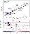 |
Fig. 9. Similar to Fig. 8 but for the comparison between seismological and astrometric masses. |
| In the text | |
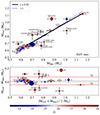 |
Fig. 10. Similar to Fig. 8 but for the comparison between spectroscopic and astrometric masses. |
| In the text | |
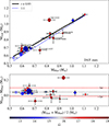 |
Fig. 11. Similar to Fig. 8 but for the comparison between photometric and astrometric masses. |
| In the text | |
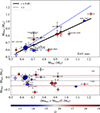 |
Fig. 12. Similar to Fig. 8 but for the comparison between seismological and photometric masses. |
| In the text | |
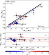 |
Fig. 13. Similar to Fig. 8 but for the comparison between spectroscopic and photometric masses. |
| In the text | |
|
Fig. 14. Comparison of stellar masses for DBV stars. Upper panel: Dispersion diagram displaying the comparison between the spectroscopic and asteroseismological masses for DBVs (see Table B.2). All the stars are identified by their names. Bottom panel: Corresponding Bland-Pearson diagram. The meaning of the different lines in both panels is the same as in Fig. 8. |
| In the text | |
|
Fig. 15. Similar to Fig. 14, this figure illustrates the comparison between spectroscopic and seismological masses, with the seismological mass derived from the period spacing (ΔΠ). It is worth noting that only seven out of the total nine DBV stars analysed have an estimate of seismological mass from the period spacing (see Table B.2). |
| In the text | |
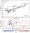 |
Fig. 16. Similar to Fig. 14 but for the comparison between the seismological and astrometric masses. |
| In the text | |
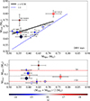 |
Fig. 17. Similar to Fig. 14 but for the comparison between spectroscopic and astrometric masses. |
| In the text | |
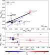 |
Fig. 18. Similar to Fig. 14 but for the comparison between spectroscopic and photometric masses. |
| In the text | |
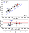 |
Fig. 19. Similar to Fig. 14 but for the comparison between photometric and astrometric masses. |
| In the text | |
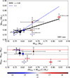 |
Fig. 20. Similar to Fig. 14 but for the comparison between seismological and photometric masses. |
| In the text | |
|
Fig. 21. Similar to Fig. 15 but for the comparison between photometric and seismological masses derived from the period spacing. |
| In the text | |
|
Fig. 22. Comparison of stellar masses for GW Vir stars. Upper panel: dispersion diagram showing the comparison between the spectroscopic and asteroseismological masses for GW Vir stars (refer to Table B.3). Stars with mass estimates that significantly disagree are annotated with their names. Bottom panel: corresponding Bland-Pearson diagram. The meaning of the different lines in both panels is the same as in Fig. 8. |
| In the text | |
|
Fig. 23. Similar to Fig. 22, this figure presents the comparison between spectroscopic and seismological masses, where the seismological masses are derived from the period spacing (ΔΠ). |
| In the text | |
|
Fig. 24. Similar to Fig. 22, this figure displays the comparison between seismological and astrometric masses. |
| In the text | |
|
Fig. 25. In analogy to Fig. 22, this figure illustrates the comparison between spectroscopic and astrometric masses. |
| In the text | |
Current usage metrics show cumulative count of Article Views (full-text article views including HTML views, PDF and ePub downloads, according to the available data) and Abstracts Views on Vision4Press platform.
Data correspond to usage on the plateform after 2015. The current usage metrics is available 48-96 hours after online publication and is updated daily on week days.
Initial download of the metrics may take a while.