| Issue |
A&A
Volume 691, November 2024
|
|
|---|---|---|
| Article Number | A115 | |
| Number of page(s) | 17 | |
| Section | Stellar structure and evolution | |
| DOI | https://doi.org/10.1051/0004-6361/202450195 | |
| Published online | 01 November 2024 | |
NSVS 14256825: Period variation and orbital stability analysis of two possible substellar companions
Department of Physics, University of Patras, 26500 Patra, Greece
⋆ Corresponding author; This email address is being protected from spambots. You need JavaScript enabled to view it.
Received:
31
March
2024
Accepted:
28
August
2024
Abstract
Context. Recent period investigations of the post-common envelop binary (PCEB) NSVS 14256825 suggest that two circumbinary companions are necessary to explain the observed eclipse timing variations (ETVs).
Aims. Our objective in this work was to search for the best-fitting curve of two LTTE terms of the ETV diagram by implementing a grid search optimization scheme of Keplerian (kinematic) and Newtonian (N-body) fits alongside a dynamical stability analysis of N-body simulations.
Methods. We compiled two datasets of archival photometric data covering different timelines and updated them with new observations and with three new times of minima calculated from the Transiting Exoplanet Survey Satellite (TESS). A grid search optimization process was implemented, and the resulting solutions that fell within the 90% confidence interval of the best-fitting curve of the ETV diagram were tested for orbital stability using N-body simulations and the MEGNO chaos indicator.
Results. The Keplerian and Netwonian fits are in close agreement, and hundreds of stable configurations were identified for both datasets reaching a lifetime of 1 Myr. Our results suggest that the ETV data can be explained by the presence of a circumbinary planet with mass mb = 11 MJup in a nearly circular inner orbit of period Pb = 7 yr. The outer orbit is unconstrained with a period range Pc = 20 − 50 yr (from 3:1 to 7:1 MMR) for a circumbinary body of substellar mass (mc = 11 − 70 MJup). The stable solutions of the minimum- and maximum-reduced chi-square value were integrated for 100 Myr and confirmed a non-chaotic behavior. Their residuals in the ETV data could be explained by a spin-orbit coupling model (Applegate-Lanza). However, continuous monitoring of the system is required in order to refine and constrain the proposed solutions.
Key words: binaries: eclipsing / planetary systems / stars: individual: NSVS 14256825
© The Authors 2024
 Open Access article, published by EDP Sciences, under the terms of the Creative Commons Attribution License (https://creativecommons.org/licenses/by/4.0), which permits unrestricted use, distribution, and reproduction in any medium, provided the original work is properly cited.
This article is published in open access under the Subscribe to Open model. This email address is being protected from spambots. You need JavaScript enabled to view it. to support open access publication.
1. Introduction
A well-known post-common envelop binary (PCEB), NSVS 14256825 (V1828 Aql, TIC 404635917) was discovered as a 13.2 mag variable star in the Northern Sky Variability Survey (NSVS) (Woźniak et al. 2004), and it has been recognized as an eclipsing binary by Wils et al. (2007) (ΔV ∼ 0.8 mag) with a very short period of P = 0.110374230(2) d and an sdOB+dM type light curve (LC; OB subdwarf and a M dwarf companion). From high precision BVRcIc LCs, Zhu et al. (2011) derived a photometric mass ratio of 0.22(0.02) and a primary mass around the value for the He core flash at M1 = 0.46 M⊙ and M2 = 0.1 M⊙ = 105 MJup for the fully convective secondary star. Almeida et al. (2012) classified NSVS 14256825 as sdOB+dM and obtained the first detailed physical and geometrical parameters from UBVRcIcJH photometric and spectroscopic observations (inclination of the system i = 82.5° ±0.3°, M2/M1 = 0.260 ± 0.0012) as M1 = 0.419 ± 0.07 M⊙, M2 = 0.109 ± 0.023 M⊙, α = 0.80 ± 0.04 R⊙ (separation between the components). Nehir & Bulut (2022), using new BVRI photometry (five nights, 2018–2019) and the old spectroscopy, presented the following updated parameters: i = 82.2° ±0.1°, M1 = 0.351 ± 0.04 M⊙, M2 = 0.095 ± 0.01 M⊙, and α = 0.74 ± 0.03 R⊙.
A large number of PCEBs show apparent period variations, which are frequently attributed to giant circumbinary planets (Zorotovic & Schreiber 2013; Heber 2016) through eclipse timing variation (ETV) caused by the light-travel time effect (LTTE) (Irwin 1952; Borkovits et al. 2015). Marsh (2018) reports at least ten PCEBs with proposed circumbinary brown dwarfs or planets detected with ETV modeling.
Zorotovic & Schreiber (2013) investigated the origin of these planets with binary population synthesis simulations and concluded that it is very unlikely that they formed in the primordial circumbinary disk (first-generation scenario) and survived the energetic common envelope (CE) evolution. The same authors proposed the formation of the planets from the CE material (second-generation scenario) as being the most likely for PCEBs, although their planetary formation is still an open question, with Bear & Soker (2014) arguing in favor of the first-generation hypothesis.
Pulley et al. (2022) evaluated seven PCEBs with claimed circumbinary planets detected using the ETV method. Remarkably, they revealed that none of the more than 30 circumbinary models that have been proposed through the years have accurately predicted eclipse times within a year. Additionally, most of these models have failed the tests of dynamic stability, making the existence of these circumbinary planets questionable. We give, as an example, HW Vir, which is the prototype of PCEBs, with a subdwarf (sdB) primary star and an M dwarf (dM) secondary. Beuermann et al. (2012a) presented a two-planetary companion model that proved to be stable for at least 10 Myr. However, recent studies (Esmer et al. 2021; Brown-Sevilla et al. 2021; Mai & Mutel 2022) have found dynamically unstable configurations on short timescales.
Notably, NSVS 14256825 has a long and conflicting history of reports of possibly having circumbinary companions, with five circumbinary models proposed in the past. Beuermann et al. (2012b) proposed an eccentric (e = 0.5) circumbinary planet of mass 12 MJ and a period of 20 yr, whereas Almeida et al. (2013) suggested a two-planetary model with masses 2.9 MJ and 8.1 MJ; periods of 3.5 yr and 6.9 yr; and eccentricities of 0.0 and 0.52 for datasets covering the time span from 1999 to 2018 and 2007 to 2012, respectively. Wittenmyer et al. (2013) ran N-body simulations for the two-planetary model and proved that it is unstable on a short timescale. Also, Hinse et al. (2014a) could not confirm the two-planetary model of Almeida et al. (2013), while their single LTTE solution was unconstrained due to a short time baseline. The ETV analysis of Nasiroglu et al. (2017) resulted in a single circumbinary brown dwarf with a of mass 15 MJ, a period of 9.9 yr, and an eccentricity of 0.175 for the time span 2007–2016. This solution is in close agreement with the results of Zhu et al. (2019) (m3 = 14.2 MJ, P3 = 8.83 yr, e3 = 0.12) and Nehir & Bulut (2022) (m3 = 13.2 MJ, P3 = 8.83 yr, e3 = 0.13) for datasets covering the time span 2008−2018 and 2007−2019, respectively. New data for the following years have indicated a divergence from these single LTTE term solutions. Wolf et al. (2021) concluded that at least two circumbinary bodies were necessary to explain the ETV data, as a single LTTE term with a period of 14 years was insufficient to fit the data. Similarly, Pulley et al. (2022) reached the same conclusion, finding that an updated ETV diagram (2007−2021) could not be adequately explained by a quadratic ephemeris and a circumbinary companion in a near circular orbit (e = 0.02) with a period of 7.65 years.
In this study, we collect all available ETV data updated with new times of minima (TOMs) calculated from the Transiting Exoplanet Survey Satellite (TESS; Ricker et al. 2015) LC data and new observations. Our objective was to search for the best-fitting curve of two LTTE terms in the ETV diagram by implementing a grid search optimization scheme alongside a dynamical stability analysis of N-body simulations, which we believe has not been attempted yet for this PCEB in this extent.
In the following section, we review alternative explanations for the ETVs in PCEBs. Then, we describe the new TOMs and the compilation of all available ETV data in Section 3. In Section 4, we analyze our search for the best-fitting curve of two LTTE terms in the ETV diagram and provide the results for different models, alongside a dynamical stability analysis and alternative mechanisms. Our discussion of the results can be found in Section 5.
2. Possible explanations for the ETVs in PCEBs
The LTTE concept faces challenges not only in terms of dynamical models for hypothetical planetary systems but also with respect to optimization techniques and phenomena inherent in the binary. Specifically, the main datasets used for ETV analyses (i.e., eclipse timings) originate from diverse sources and methods, involve various software packages and algorithms, and are often accompanied by underestimated errors (Pribulla et al. 2012).
Alternative mechanisms have been proposed as explanations for the apparent ETV variations, such as mass transfer, apsidal motion (Lacy 1992), magnetic effects (Applegate 1992; Völschow et al. 2016; Lanza 2020), and angular momentum loss through gravitational radiation (Paczyński 1967) or magnetic breaking (Rappaport et al. 1983) in one or both stars. Since sdB binaries are detached systems, mass transfer cannot occur. Apsidal motion would not be expected in PCEBs with α < 1 R⊙; thus the orbit can be considered circular (e = 0), and the rotation of the components synchronized with the orbit. Parsons et al. (2014) suggest that orbital eccentricities much less than 0.001 can introduce a maximum ETV of 5.5 s (for P ∼ 0.1 d), and thus it is considered a minor contributing factor to the observed ETVs. However, apsidal motion is the combined result of perturbations of a Keplerian orbit that include tidal and rotational contributions, a general relativity contribution, and possibly a third-body contribution. Analytical formulae can be found in Parsons et al. (2014), Bulut et al. (2017), Almeida et al. (2020), Dimoff & Orosz (2023). Due to their proximity, PCEBs frequently undergo complex gravitational effects that depart from idealized spherical models. Due to dynamic interactions between the stars as they evolve and lose their spherical symmetry, caused by factors such as rotation, magnetic fields, and tidal forces, precession of the orbits may result. In situations, where the gravitational term is not taken into account, the rate of apsidal motion can be used as a probe of the internal structure of the stars. At the same time, although it was not ruled out, Almeida et al. (2020) discovered that apsidal motion due to tidal and rotation effects was less plausible than substellar component models in the case of the PCEB GK Vir. Therefore, we do not take this effect into further consideration in the current investigation.
Because of the small masses, barely any recorded ETV signals may be attributed to gravitational radiation despite the short orbital periods. Considering the high surface gravities of the components, star winds should also be extremely weak and make minimal contributions. Given that the secular variations can occur at a timescale significantly longer than the baseline of data, it is very easy to confuse periodic changes with the former. The overall cyclical behavior of ETV cannot be explained by angular momentum loss (AML) from magnetic braking or gravitational radiation, which drives the binary to a constant reduction in the period without a quasi-cyclical component.
Magnetic activity cycles of the secondary components can imitate ETV behavior provided that the star has a sufficient energy budget (Applegate mechanism). According to the Applegate model (Applegate 1992) a magnetic active star in a binary can transfer angular momentum toward the surface from its interior and away from it during a complete magnetic cycle, leading to oscillations of the orbital period. The magnetic star’s energy budget must be sufficient to adjust its quadrupole moment for this mechanism to work, resulting in a variable luminosity. Völschow et al. (2016) proposed a more accurate and realistic two-zone model where they treated a stellar density profile of the inner and outer regions for two different densities, including the change of the quadrupole moment both in the shell and the core, adding to previous improvements of the mechanism (Lanza & Rodonò 2004; Brinkworth et al. 2006; Lanza 2006; Tian et al. 2009). A novel model has been developed recently by Lanza (2020). It is based on the exchange of angular momentum between the binary orbital motion and the spin of the magnetically active secondary. This mechanism could help explain the observed ETVs and potentially get over the original Applegate mechanism’s energy constraints. Although these alternatives often fail to explain the magnitude of the observed ETVs or to satisfy the required observational evidence of each mechanism (Pulley et al. 2022) in most cases, their contribution can become significant (RR Cae, DE CVn; Pulley et al. 2022).
3. Data acquisition
We compiled 305 eclipse minimum times from the literature as follows: 152 from Table 4 of Nasiroglu et al. (2017) (these include 18 by Wils et al. 2007, 32 by Beuermann et al. 2012b, nine by Kilkenny & Koen 2012, and ten by Almeida et al. 2012); 84 by Zhu et al. (2019), 41 by Wolf et al. (2021), 20 by Pulley et al. (2022), and eight by Nehir & Bulut (2022) (only the primaries). All TOMs are in BJD-TDB. Details of the observations (error, eclipse type, observatory) can be found in the papers mentioned. In addition, we updated the TOMs with our own observations carried out in 2017 using the 14-inch Schmidt-Cassegrain telescope at the Patras University “Mythodea” Observatory (Papageorgiou & Christopoulou 2015a). Three new TOMs were calculated from TESS sector 51 with a 2-min cadence for the year 2022, available from the Mikulski Archive for Space Telescopes (MAST)1, and two new TOMs were collected from the online B.R.N.O.2 database during the years 2023 and 2024 (Table 1).
New times of minimum light for NSVS 14256825.
Our own observations were taken with an RC filter. The standard processes of bias subtraction, flat fielding, and dark subtraction were used to reduce the CCD frames. Differential magnitudes were obtained by choosing a non-variable star in the field of view comparable to the target in brightness (GSC 00504 00639) and a comparison star (2MASS 1084555518). Image reduction and differential photometry were performed using a fully automated pipeline (Papageorgiou & Christopoulou 2015b) that incorporates Pyraf (Science Software Branch at STScI 2012) and the Astrometry.net packages (Lang et al. 2010).
The TESS LC in Fig. 1a was plotted with normalized SAP fluxes of the best quality (quality flag zero) data points using the Lightkurve Python package for Kepler and TESS data analysis Lightkurve Collaboration (2018), from which we generated a phased-folded and binned LC (FBLC) for each time series segment (Fig. 1b). Employing a modified Kwee–Van Woerden (Deeg 2020) method for eclipse minimum timing with reliable error estimates, one primary TOM was calculated from each FBLC following the process of TOM determination described in Zervas et al. (2024). All the HJD times were transformed into TDB-based BJD ones by using the publicly available code of Eastman et al. (2010).
 |
Fig. 1. (a) TESS LC time series composed of three segments (sector 51), (b) phase-folded binned LCs for each segment. |
A total of 312 TOMs were used in the ETV analysis (Table B.1), excluding low-precision timings and using only the timings with errors smaller than ∼17 s (0.0002 d). Consistent with previous data categorizations (Beuermann et al. 2012b; Nasiroglu et al. 2017; Pulley et al. 2022), we established two datasets. The first one includes the less precise NSVS and All Sky Automated Survey (ASAS) data, offering a broader time frame from 1999 to 2024 (dataset A), while the second one with 307 TOMs excludes these data, narrowing down the analysis to the years 2007 to 2024 (dataset B). Using the linear part of ephemeris from Pulley et al. (2022),
 (1)
(1)
we calculated and plotted the ETV diagram (Fig. 2) of each dataset.
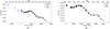 |
Fig. 2. ETV diagrams of NSVS 14256825. (a) ETV diagram of dataset A spanning 26 years (1999–2024). Archival data ∼black open circles; NSVS+ASAS data ∼blue open circles; Mythodea data ∼orange open circles; TESS data ∼green open circles; B.R.N.O. data ∼red open circles. (b) ETV diagram of dataset B spanning 18 years (2007–2024). Color indexing is the same as in (a). |
4. Analysis and results
4.1. Analysis outline
We adopted the formulation of Goździewski et al. (2012) for the LTTE term:
![Mathematical equation: $$ \begin{aligned} \mathrm{LTTE}_{p}= K_p \left[\sin \omega _{p} \cos (E_p(t)-e_p)+\cos \omega _{p} \sqrt{1-e_{p}^2} \sin E_p(t)\right], \end{aligned} $$](/articles/aa/full_html/2024/11/aa50195-24/aa50195-24-eq2.gif) (2)
(2)
where Kp, ep, ωp are the semi-amplitude of the LTTE signal, eccentricity, and argument of the pericenter, respectively, for body p (p = b, c for inner and outer orbit, in accordance with the common convention). The orbital period Pp and the pericenter passage Tp depend on the eccentric anomaly Ep(t), and hence they do not explicitly appear in Equation (2). This is a revised kinematic (Keplerian) formulation of the LTTE effect (Irwin 1952) for multiple circumbinary companions, where the eclipse ephemerides is expressed with regard to Jacobi coordinates, with the origin at the center of mass (CM) of the binary.
According to Goździewski et al. (2012), the osculating orbital elements and masses derived with this revised formulation best match the true N-body initial condition of the system with mutually interacting planets. However, these Keplerian orbits are only an approximation of the true (Newtonian) orbits in the case of more than two bodies, and as a result, one needs to determine whether the degree of approximation is significant. This discrepancy has been highlighted first in radial velocity studies of extrasolar planets (Laughlin & Chambers 2001; Goździewski et al. 2003) and becomes substantial in cases of massive, strongly interacting planets close to low-order mean motion resonances (MMRs).
In total, our least-squares fit involves twelve parameters: two for the linear ephemeris of the binary (the epoch T0 and period Pbin) and five orbital elements for each body (ep, Pp, ωp, Tp, αp), where αp is the semi-major axis and p = b, c for each LTTE orbit. We followed a grid search approach similar to that of Beuermann et al. (2013). Our optimization process consisted of two sets of runs in the eb, ec plane utilizing a combination of the Nelder-Mead Simplex and Levenberg-Marquardt algorithms using the LMFIT Python package (Newville et al. 2023). The goal was to identify the best-fitting curve in the ETV diagram of models featuring two LTTE terms.
Additionally, each solution that achieved a reduced chi-square (χν2) value below a preset limit (listed below) was integrated with the REBOUND N-body code (Rein & Liu 2012) using the IAS15 integrator (Rein & Spiegel 2015), requiring a lifetime τ = 1 Myr and a MEGNO chaos indicator (Cincotta et al. 2003) value ⟨Y⟩∼2 as an additional acceptance criterion. Therefore, an acceptable model can be considered one that provides a good fit to the data and is secularly stable with non-chaotic orbital behavior.
This optimization process was independently applied to two distinct ETV datasets (dataset A, dataset B), each covering a different time span. The initialization of each integration was set up with the transformation of the initial condition from the Jacobian kinematic frame to the N-body Cartesian osculating frame, with the origin at the CM, at the osculating epoch T0. Furthermore, we used these initial conditions and refined them in terms of the exact N-body model. An iterative Levenberg-Marquardt process was implemented, and we examined how the χν2 value of the fit depends on variations of all orbital elements (Laughlin & Chambers 2001). In that way, a fully self-consistent Newtonian fit to the ETV data could be made.
Figure 3 illustrates the difference between the synthetic LTTE signals of a Jacobian (Keplerian) and an N-body (Newtonian) fit for dataset A. The maximum time difference of 1.2 sec is comparable to the discrepancy of Keplerian and Newtonian two-planet models for the ETV diagram of the post-common envelope binary NN Ser, as has been shown in Marsh et al. (2014), while these differences are about ten times larger for the cataclysmic binary HU Aqr (Goździewski et al. 2015).
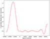 |
Fig. 3. Differences of the LTTE signals derived from a typical Jacobian fit and from respective osculating N-body models integrated numerically with the inferred initial condition at the osculating epoch T0 = 54274.20875 BJD of the zeroth cycle, where the two models seem to agree. |
The steps of the fitting process are outlined as follows:
-
Run 1: Grid search optimization in the eb, ec plane with fixed eccentricity values in the range [0, 0.98] and a step size of 0.01 (9801 models). The rest of the parameters were subsequently optimized, initiating from values chosen randomly within physically accepted limits.
-
Run 2: The resulting solutions of Run 1 served as the initial points for a new optimization run. However, this time all the parameters, including eccentricities, were adjusted during the fitting process.
-
N-body simulations for 1 Myr of the obtained Keplerian solutions of both runs while selectively excluding models that deviate beyond the 90% confidence level of the reduced chi-square (χν2) for two degrees of freedom in order to acquire well-fitted curves. Specifically, we considered solutions with χν2 ≤ χν, best2 + Δχ, where χν, best2 corresponds to the chi-square value of the best-fitting curve and Δχ = 4.6.
-
Self-consistent N-body (Newtonian) orbital fits initialized from each Keplerian fit of step 3 and subsequent integrations for 1 Myr.
In the first optimization run (Run 1), the eccentricities are fixed, and the rest of the parameters are free to adjust, while in the second run (Run 2), all parameters are allowed to vary. Throughout all orbital simulations, we treated the central binary as a single object and considered only co-planar, edge-on cases. This is the simplest scenario, and it is commonly assumed in stability analyses of exoplanets, as it minimizes the masses of the planets relative to the binary, thereby promoting stability (Beuermann et al. 2012a; Horner et al. 2012; Marsh et al. 2014; Mai & Mutel 2022; Esmer et al. 2023). However, there are cases, such as the putative HU Aqr planetary system, that appear to be more complex (highly non-coplanar), resulting in stable orbits in contrast to the co-planar scenario (Goździewski et al. 2015). Fundamental parameters of the binary are from Nehir & Bulut (2022) and were used for the rest of the analysis when needed.
4.2. Period variation and orbital stability
Optimization results of Keplerian models are shown in Tables 2 and 3 for each dataset and Runs 1 and 2, respectively. Each optimization run is characterized by three critical values: the best reduced chi-square value (χν, best2) of the best-fitting curve to ETV data and the minimum- (χν, min2) and the maximum-reduced chi-square (χν, max2) values among all stable solutions. The same description is followed in Tables 4, 5 for the Newtonian models. The reported parameter uncertainties correspond to the standard 1-σ error, and their calculation resulted from the covariance matrix.
Grid search optimization results of Keplerian two-planet LTTE fit after Run 1 of the fitting process for both datasets (A and B).
Grid search optimization results of Keplerian two-planet LTTE fit after Run 2 of the fitting process for both datasets (A and B).
Self-consistent Newtonian two-planet orbital fits initialized from the results of optimization Run 1 for both datasets (A and B).
Self-consistent Newtonian two-planet orbital fits initialized from the results of optimization Run 2 for both datasets (A and B).
It is notable that none of the best-fitting curves (χν, best2) are stable for more than a few hundred years. However, there are hundred of stable orbits (τ = 1 Myr, ⟨Y⟩∼2) within the 90% confidence level of each of the best reduced chi-square values. Illustrated in Fig. 4 are the lifetime distributions of eccentricities as well as the periods and the fitting curves corresponding to the three critical cases of Keplerian (Fig. 5) and Newtonian (Fig. A.4) models for each dataset.
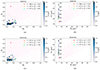 |
Fig. 4. Top: Lifetime colormap plots in the (a) eb, ec and (b) Pb, Pc planes for 5838 Keplerian models (99 stable) within the 90% confidence level of χν, best2 as they resulted from optimization Run 1 for dataset A. Bottom: Same as top but for 5838 Newtonian models (74 stable). The color coding displays the range of lifetimes from white to dark blue, while the orange and green crosses correspond to the positions of the minimum- and maximum-reduced chi-square value of the stable configurations. The best-fitting curve to the data is identified by the red cross, which is unstable in all cases. The MMR solutions have been labeled in the Pb, Pc plane for the nominal Pb = 7 yr. |
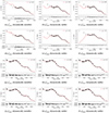 |
Fig. 5. Keplerian fits for both datasets [A: (a)–(f), B: (g)–(l)] and optimization runs [1: (a)–(c), (g)–(i), 2: (d)–(f), (j)–(l)]. The best-fitting curves (χν, best2) result in dynamically unstable configurations, while the fitting curves of the minimum- and maximum-reduced chi-square value (χν, min2, χν, max2) define the χν2 limits among all stable configurations. The parameters of each case can be found in Tables 2 and 3. |
For dataset A, 99 stable Keplerian orbits and 74 stable Newtonian orbits were found among 5838 models, each with a chi-square value falling within the 90% confidence level of the best-fitting curve (χν, best2 = 5.26) during optimization Run 1. Subsequently, following optimization Run 2, 153 stable Keplerian orbits and 93 stable Newtonian orbits were identified out of 8123 models, all meeting the same criteria.
Similarly, in dataset B, after optimization Run 1, we found 198 stable Keplerian orbits and 171 stable Newtonian orbits among 6055 models, each with a chi-square value lying within the 90% confidence level of the best-fitting curve (χν, best2 = 5.76). The greatest number of stable solutions was discovered after optimization Run 2 of dataset B, revealing 454 stable Keplerian orbits and 423 stable Newtonian orbits among 8216 models, all having reduced chi-square values within the 90% confidence level of χν, best2 = 5.26.
The lifetime distributions of Pb, Pc (subplots b and d of Figs. 4, A.3) reveal the existence of a constrained inner orbit with period Pb = 7 yr and an unconstrained outer orbit with periods in the range of 3:1 to 7:1 MMR. The same conclusion about the constrained (unconstrained) inner (outer) orbits can be deduced by the histograms of the Keplerian (Figure A.5) and Newtonian (Figure A.6) models for both datasets.
Both datasets seem to constrain the inner planet to a nearly circular orbit with a mean period of Pb ∼ 7 yr, while the outer companion has a circular orbit for either dataset and optimization run. When comparing the mean outer periods across datasets and optimization runs, a noticeable deviation of almost 27 years was observed between the two datasets of optimization Run 1 (Figures A.5d, A.6d), while this discrepancy decreases to a deviation of at least seven years for the results of optimization Run 2 (Figures A.5h, A.6h). Nevertheless, the well-defined peak in the outer period histograms of dataset A suggests a more constrained outer period with a mean value of Pc ∼ 23 yr, in contrast to the broader distributions of dataset B with a mean value of Pc ∼ 40 yr.
The N-body osculating initial conditions derived from the kinematic (Keplerian) fits provide χν2 values that are comparable with the Jacobian solutions. Figure 6 illustrates a kinematic model and its formal transformation to the N-body Cartesian osculating frame, from which Figure 3 was produced. Similarly, the refined self-consistent N-body solutions result in χν2 values comparable to those of the Keplerian fits. The only exception is the χν, max2 solutions of optimization Run 1 (Tables 2, 4), which is justified because the eccentricities of self-consistent N-body models oscillate, in contrast to their fixed values in Run 1. Therefore, the kinematic solutions and the transformed kinematic initial conditions are as consistent with the observations as the self-consistent Newtonian fits.
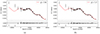 |
Fig. 6. ETV diagrams with synthetic curves. Left: Keplerian fit of two-planet Jacobian solution (Table 2, χν, min2, dataset A). Right: N-body synthetic curve for the osculating initial condition derived through the formal transformation of the Jacobian elements (Keplerian fit) to the N-body Cartesian osculating frame, centered at the CM of the binary. |
We investigated further the orbital stability of the eight critical solutions (χν, min2, χν, max2 of both datasets and all optimization runs) by integrating each one for 100 Myr. All orbits were found to be stable in this timescale, which is considered the lifetime of the PCEB phase of sdB binaries (King & Schenker 2002; Schreiber & Gänsicke 2003). In Fig. 7, we plot indicatively the orbital evolution of eccentricities and semi-major axes, initialized by a Keplerian solution (Table 2, dataset B, χν, min2), over 100 Myr.
Additionally, in Fig. 7c, we display the LTTE effect of this indicative solution for the first 152 years, phase folded in the ETV diagram. Each synthetic curve corresponds to an integration time equal to the outer period (38 years). The black synthetic curve is the Keplerian (kinematic) fit, which appears to be in absolute agreement with the dynamical fit for the first 38 years (green curve). The rest of the synthetic curves are also in close agreement with the initial Keplerian fit. This allowed us to test the validity of the Keplerian fits to the data.
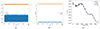 |
Fig. 7. Orbital evolution of (a) eccentricities and (b) semi-major axes for the inner and outer planets over 100 Myr (dataset B, Run 1, χν, min2). (c) The temporal variation of the χν, min2 fitting curve (dataset B, Run 1) over the first 152 years is represented by five sets of parameters, each corresponding to a complete outer orbit revolution (38 years). The black synthetic curve is the Keplerian (kinematic) fit from which this dynamical model was initialized, and it appears to be in absolute agreement with the first 38 years of orbital evolution (green curve) and in close agreement with the subsequent fits (blue and red curves). |
Finally, in Fig. 8 we plot the temporal evolution of the mean-motion resonant angles θ1 = 3λo − λi − 2ϖi, θ2 = 3λo − λi − 2ϖo, and θ3 = 3λo − λi − ϖi − ϖo (Beaugé et al. 2003; Michtchenko et al. 2008) for the first 10 000 years of a stable solution close to 3:1 MMR (Table 2, χν, min2, dataset A). It is apparent that these critical angles librate around zero degrees, indicating a dynamical resonant system.
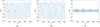 |
Fig. 8. Temporal evolution of resonant angles (a) θ1, (b) θ2, and (c) θ3 of a stable solution close to the 3:1 MMR (Table 2, χν, min2, dataset A) over the first 10 000 years of integration. |
4.3. Alternative explanations for ETV
We have investigated if the cyclic period modulation can also be driven by magnetic activity cycles (Applegate 1992) of the secondary component of NSVS 14256825, as it is a convective red dwarf star with an effective temperature of 3077 K and a mass of 0.095 M⊙ (Nehir & Bulut 2022). Using the online tool of Völschow et al. (2016)3, we calculated the energy demand (ΔE/E2) for two different models: (i) the finite-shell two-zone model (Völschow et al. 2016) and (ii) the thin-shell model (Tian et al. 2009). We also calculated the requirements for the spin-orbit coupling model (Lanza 2020). To explain the observed ETV modulation, the magnetic activity of the secondary must meet the criterion (ΔE/E2 ≪ 1) for the energy demand. All the calculated energy ratios for a period modulation of 7 to 48 yr were found to be larger than the threshold. Thus, we investigated the requirements for the spin-orbit coupling model (Applegate-Lanza) to account for residual changes in the O-C stable model fits. For the two datasets, A and B, these are 22 s and 43 s over T = 18 yr and T = 26 yr, respectively. Following the rationale of the equations of Mai & Mutel (2022) and Lanza (2020), the change in rotational energy ΔErot ∼ −(2 − 3)×1032 J is smaller than the maximum energy available (4.4 − 6.3)×1032 J from luminosity changes over the timescale for O-C variability in the secondary star Emax = L2 × T. Therefore, ΔErot/Emax is ∼0.5, and it could account for the residual changes in the ETV model fits. Given the spectral type M5-M8 for the secondary of NSVS 14256825, this is in agreement with the conclusion of Bours et al. (2016) that as magnetic activity decreases toward a later spectral type, we expect to drive much smaller O-C variations. Nevertheless it is still a high number, meaning that half of the energy generated by the secondary star should account for the non-axisymmetric gravitational quadrupole moment. We also calculated the tidal synchronization timescale following the assumptions and equations of Lanza (2020) and found ts = 3.4 − 34 yr for the dimensionless tidal quality factor Q = 105 − 106 that respectively characterizes the efficiency of tidal energy dissipation in the active (secondary) component. As these times are similar to the observed O-C changes, the timescale for spin-orbit coupling may be determined by tidal synchronization instead of by magnetic activity timescales.
5. Discussion and conclusions
We implemented a grid search approach consisting of two sets of optimization runs (Run 1: for fixed eccentricities, Run 2: adjusting all resulting parameters from Run 1) in the eb, ec plane utilizing a combination of the Nelder-Mead Simplex and Levenberg-Marquardt algorithms. The goal was to find the best-fitting curve (χν, best2) in the ETV diagram of two datasets (dataset A, dataset B), implementing a revised kinematic (Keplerian) formulation of the LTTE effect and self-consistent N-body (Newtonian) models. Additionally, we ran three-body simulations of the resulting solutions that lie within the 90% confidence interval of the best-fitting curve, searching for stable (τ = 1 Myr) and non-chaotic (⟨Y⟩∼2) orbits.
As a result, hundreds of stable orbits, with a lifetime of at least 1 Myr, were found for two circumbinary bodies of substellar mass within the 90% confidence interval of the best-fitting curve. However, none of the Keplerian and Newtonian χν, best2 solutions were dynamically stable for more than a few hundred years. The histograms and lifetime distributions of inner and outer periods revealed the existence of a constrained inner orbit with period Pb = 7 yr, mass mb = 11 MJup, and an unconstrained outer orbit with a period in the range of 3:1 to 7:1 MMR (Pc = 20 − 50 yr) and a mass range of mc = 11 − 70 MJup. Recent ETV studies of multiple-planet systems have reported that orbits close to low-order MMRs are strongly unstable (Horner et al. 2012; Goździewski et al. 2015; Hinse et al. 2014b; Esmer et al. 2021) for timescales as short as thousands of years. The only exception based on ETV analysis is NY Vir (Esmer et al. 2023), with a period variation attributed to two putative Jovian planets close to 2:1 MMR, although this is uncertain due to the short time interval of the observations.
Furthermore, the observational timeline of ETV diagrams are usually narrow relative to the putative orbital periods, and as a consequence, the inferred masses of hypothetical planets reach the brown dwarf and the red dwarf limits (Hinse et al. 2012; Goździewski et al. 2015). Such cases may introduce significant deviations between synthetic signals derived from the Keplerian and osculating Newtonian elements, leading to qualitatively different best-fitting configurations constrained by the available data. In the case of NN Ser, the Newtonian fits of Marsh et al. (2014) are in qualitative agreement with the Keplerian fits of Beuermann et al. (2013). However, the following analyses (Bours et al. 2016; Pulley et al. 2022; Özdönmez et al. 2023) of the system revealed that the initially stable system in 2:1 MMR does not fit the updated time measurements. Here, both datasets confirm the presence of a circumbinary planet with Pb ∼ 7 yr, but deviations in the outer period were observed: Pc ∼ 23 yr for dataset A and Pc ∼ 40 yr for dataset B. This discrepancy suggests that the extended timeline of dataset A, spanning 26 years, may provide better constraints on the orbital parameters compared to the narrower 18-year time frame of dataset B.
In any case, the fitting curves of stable orbits are not perfectly fitted to the complete datasets in comparison to the best-fitting curves. The low precision NSVS and ASAS data seem to follow the general trend of strong peak-to-peak amplitude reduction over time, although the fitting curves of the minimum- and maximum-reduced chi-square of stable solutions do not fit well within their respective time frames (1999−2007). Moreover, both datasets exhibit visually similar fits for the minimum- (χν, min2) and maximum-reduced (χν, max2) chi-square of stable solutions in the 2007−2024 interval, but they do not fit perfectly through the latest data of 2021−2024. In general, the self-consistent N-body models account for mutual gravitational interactions between the circumbinary bodies, which could affect the ETV trends. We showed that the temporal variation of the mid-eclipse times of the binary, as predicted by a best-fitting dynamical two-planet model, are in close agreement with the initial Keplerian fit. In addition, our Keplerian fits produce qualitatively the same results as the Newtonian ones. As a result, we attribute these ETV residuals to the sparse data of the corresponding time frames and/or additional mechanisms (Applegate-Lanza, spin-orbit coupling model). We applied the model of Lanza (2020), and although it depends on poorly constrained binary system parameters, such as the tidal energy dissipation and the internal mass distribution of the stars, we found that it may contribute to the observed ETV, apart from the potential circumbinary bodies, revealing the complex nature of the orbital structure of NSVS 14256825, as in the case of HS 0705+6700 (Mai & Mutel 2022) and V471 Tau (Kundra et al. 2022).
The plentiful stable solutions that were found, coupled with their relatively well-fitted ETV curves, could serve as evidence supporting the existence of two circumbinary companions of substellar mass orbiting NSVS 14256825. We also tested the stability of the eight critical stable solutions (χν, min2, χν, max2 of both datasets and of both optimization runs) for an integration interval of 100 Myr. All of these solutions were found to be stable in this timescale, which is considered to be the lifetime of the PCEB phase of sdB binaries.
We could not suggest one conclusive model of two circumbinary planets since one cannot rely solely on the statistics of a reduced chi-square. Regarding the reduced chi-square for each dataset and optimization run, the eight critical stable solutions outline the extrema of a group of solutions. However, within these limits exist hundreds of solutions with various parameter values that are not centered around a best-fit solution. Dataset A seems to constrain the model parameters for both companions, but the fitting curves of the critical stable solutions are far from satisfactory for the earliest NSVS and ASAS data. On the other hand, dataset B provides more satisfactory fits, but there are cases where the mean outer period exceeds 30 years in both optimization runs and the inferred masses reach values greater than 30 MJup.
Among the ten PCEBs exhibiting LTTE signals (for the complete list, refer to Pulley et al. 2022), half of them (HW Vir, NY Vir, NN Ser, HS 0705+6700, Kepler-451) exhibit two or more cyclic variations attributed to circumbinary planets. Their ETV and dynamical stability analyses share some common features, among which are the continuously updated LTTE solutions, peak-to-peak amplitude reduction (Pulley et al. 2022), and stable regions of higher χ2 than the best-fit solution (Potter et al. 2011; Dreizler et al. 2012; Esmer et al. 2022; Özdönmez et al. 2023). From our analysis, it seems that NSVS 14256825 is not an exception.
We examined the potential for detecting the planets of ETV using Gaia (DR3; Gaia Collaboration 2023) astrometry. The detection limit of an outer planet can be calculated by following the formalism of Sahlmann et al. (2015) and the NSVS 14256825 distance, 752.6 pc according to the Gaia DR3 parallax measurements. Among the stable models, using the masses and the periods of, for example, the χν, max2 dataset B (Run 2) solution (mb = 11.12 MJ, Pb = 7.04 yr, mc = 8.57 MJ, Pc = 24.91 yr), the gravitational pull of the planet will displace the system’s barycenter, with a semi-major axis of ab ∼ 19 mas and ac ∼ 34 mas, respectively. This represents the planet’s astrometric signature, which to be detectable must be greater than the scan length accuracy per optical field pass σfov corresponding to the luminosity G (Perryman et al. 2014). For the NSVS 14256825 (G = 13.22) σfov ∼ 42 μas, and thus Gaia can detect the planets of NSVS 14256825.
As recently proposed for the case of HW Vir by Baycroft et al. (2023), Gaia full-epoch astrometry (circa 2025) will provide an alternative method to ETVs for confirming circumbinary planets of PCEBs. In the meantime, it is essential to continue monitoring the system in order to expand the observational timeline with new data, providing further validation and refinement of the proposed solutions.
Acknowledgments
We thank the anonymous referee for numerous constructive comments and suggestions that greatly improved this paper.
References
- Almeida, L. A., Jablonski, F., Tello, J., & Rodrigues, C. V. 2012, MNRAS, 423, 478 [Google Scholar]
- Almeida, L. A., Jablonski, F., & Rodrigues, C. V. 2013, ApJ, 766, 11 [Google Scholar]
- Almeida, L. A., Pereira, E. S., Borges, G. M., et al. 2020, MNRAS, 497, 4022 [Google Scholar]
- Applegate, J. H. 1992, ApJ, 385, 621 [Google Scholar]
- Baycroft, T. A., Triaud, A. H. M. J., & Kervella, P. 2023, MNRAS, 526, 2241 [CrossRef] [Google Scholar]
- Bear, E., & Soker, N. 2014, MNRAS, 444, 1698 [CrossRef] [Google Scholar]
- Beaugé, C., Ferraz-Mello, S., & Michtchenko, T. A. 2003, ApJ, 593, 1124 [Google Scholar]
- Beuermann, K., Dreizler, S., Hessman, F. V., & Deller, J. 2012a, A&A, 543, A138 [NASA ADS] [CrossRef] [EDP Sciences] [Google Scholar]
- Beuermann, K., Breitenstein, P., Debski, B., et al. 2012b, A&A, 540, A8 [NASA ADS] [CrossRef] [EDP Sciences] [Google Scholar]
- Beuermann, K., Dreizler, S., & Hessman, F. V. 2013, A&A, 555, A133 [NASA ADS] [CrossRef] [EDP Sciences] [Google Scholar]
- Borkovits, T., Rappaport, S., Hajdu, T., & Sztakovics, J. 2015, MNRAS, 448, 946 [NASA ADS] [CrossRef] [Google Scholar]
- Bours, M. C. P., Marsh, T. R., Parsons, S. G., et al. 2016, MNRAS, 460, 3873 [Google Scholar]
- Brinkworth, C. S., Marsh, T. R., Dhillon, V. S., & Knigge, C. 2006, MNRAS, 365, 287 [Google Scholar]
- Brown-Sevilla, S. B., Nascimbeni, V., Borsato, L., et al. 2021, MNRAS, 506, 2122 [NASA ADS] [CrossRef] [Google Scholar]
- Bulut, İ., Bulut, A., & Demircan, O. 2017, MNRAS, 468, 3342 [Google Scholar]
- Cincotta, P. M., Giordano, C. M., & Simó, C. 2003, Phys. D Nonlinear Phenom., 182, 151 [Google Scholar]
- Deeg, H. J. 2020, Galaxies, 9, 1 [NASA ADS] [CrossRef] [Google Scholar]
- Dimoff, A. J., & Orosz, J. A. 2023, AJ, 166, 114 [NASA ADS] [CrossRef] [Google Scholar]
- Dreizler, S., Beuermann, K., & Hesman, F. V. 2012, Mem. Soc. Astron. It., 83, 498 [NASA ADS] [Google Scholar]
- Eastman, J., Siverd, R., & Gaudi, B. S. 2010, PASP, 122, 935 [Google Scholar]
- Esmer, E. M., Baştürk, Ö., Hinse, T. C., Selam, S. O., & Correia, A. C. M. 2021, A&A, 648, A85 [NASA ADS] [CrossRef] [EDP Sciences] [Google Scholar]
- Esmer, E. M., Baştürk, Ö., Selam, S. O., & Aliş, S. 2022, MNRAS, 511, 5207 [NASA ADS] [CrossRef] [Google Scholar]
- Esmer, E. M., Baştürk, Ö., & Selam, S. O. 2023, MNRAS, 525, 6050 [NASA ADS] [CrossRef] [Google Scholar]
- Gaia Collaboration (Vallenari, A., et al.) 2023, A&A, 674, A1 [NASA ADS] [CrossRef] [EDP Sciences] [Google Scholar]
- Goździewski, K., Konacki, M., & Maciejewski, A. J. 2003, ApJ, 594, 1019 [CrossRef] [Google Scholar]
- Goździewski, K., Nasiroglu, I., Słowikowska, A., et al. 2012, MNRAS, 425, 930 [NASA ADS] [CrossRef] [Google Scholar]
- Goździewski, K., Słowikowska, A., Dimitrov, D., et al. 2015, MNRAS, 448, 1118 [CrossRef] [Google Scholar]
- Heber, U. 2016, PASP, 128, 082001 [Google Scholar]
- Hinse, T. C., Goździewski, K., Lee, J. W., Haghighipour, N., & Lee, C.-U. 2012, AJ, 144, 34 [NASA ADS] [CrossRef] [Google Scholar]
- Hinse, T. C., Lee, J. W., Goździewski, K., Horner, J., & Wittenmyer, R. A. 2014a, MNRAS, 438, 307 [Google Scholar]
- Hinse, T. C., Horner, J., & Wittenmyer, R. A. 2014b, J. Astron. Space Sci., 31, 187 [NASA ADS] [CrossRef] [Google Scholar]
- Horner, J., Hinse, T. C., Wittenmyer, R. A., Marshall, J. P., & Tinney, C. G. 2012, MNRAS, 427, 2812 [Google Scholar]
- Irwin, J. B. 1952, ApJ, 116, 211 [Google Scholar]
- Kilkenny, D., & Koen, C. 2012, MNRAS, 421, 3238 [Google Scholar]
- King, A. R., & Schenker, K. 2002, ASP Conf. Ser., 261, 233 [NASA ADS] [Google Scholar]
- Kundra, E., Hambálek, Ľ., Vanaverbeke, S., et al. 2022, MNRAS, 517, 5358 [NASA ADS] [CrossRef] [Google Scholar]
- Lacy, C. H. S. 1992, AJ, 104, 2213 [NASA ADS] [CrossRef] [Google Scholar]
- Lang, D., Hogg, D. W., Mierle, K., Blanton, M., & Roweis, S. 2010, AJ, 139, 1782 [Google Scholar]
- Lanza, A. F. 2006, MNRAS, 369, 1773 [NASA ADS] [CrossRef] [Google Scholar]
- Lanza, A. F. 2020, MNRAS, 491, 1820 [NASA ADS] [Google Scholar]
- Lanza, A. F., & Rodonò, M. 2004, Astron. Nachr., 325, 393 [NASA ADS] [CrossRef] [Google Scholar]
- Laughlin, G., & Chambers, J. E. 2001, ApJ, 551, L109 [CrossRef] [Google Scholar]
- Lightkurve Collaboration (Cardoso, J. V. D. M., et al.) 2018, Astrophysics Source Code Library [record ascl:1812.013] [Google Scholar]
- Mai, X., & Mutel, R. L. 2022, MNRAS, 513, 2478 [NASA ADS] [CrossRef] [Google Scholar]
- Marsh, T. R. 2018, in Handbook of Exoplanets, eds. H. J. Deeg, & J. A. Belmonte, 96 [Google Scholar]
- Marsh, T. R., Parsons, S. G., Bours, M. C. P., et al. 2014, MNRAS, 437, 475 [NASA ADS] [CrossRef] [Google Scholar]
- Michtchenko, T. A., Beaugé, C., & Ferraz-Mello, S. 2008, MNRAS, 387, 747 [NASA ADS] [CrossRef] [Google Scholar]
- Nasiroglu, I., Goździewski, K., Słowikowska, A., et al. 2017, AJ, 153, 137 [Google Scholar]
- Nehir, Ç., & Bulut, İ. 2022, New Astron., 92, 101703 [NASA ADS] [CrossRef] [Google Scholar]
- Newville, M., Otten, R., Nelson, A., et al. 2023, https://doi.org/10.5281/zenodo.598352 [Google Scholar]
- Özdönmez, A., Er, H., & Nasiroglu, I. 2023, MNRAS, 526, 4725 [CrossRef] [Google Scholar]
- Paczyński, B. 1967, Acta Astron., 17, 287 [NASA ADS] [Google Scholar]
- Papageorgiou, A., & Christopoulou, P. E. 2015a, AJ, 149, 168 [NASA ADS] [CrossRef] [Google Scholar]
- Papageorgiou, A., & Christopoulou, P. E. 2015b, ASP Conf. Ser., 496, 181 [NASA ADS] [Google Scholar]
- Parsons, S. G., Marsh, T. R., Bours, M. C. P., et al. 2014, MNRAS, 438, L91 [NASA ADS] [CrossRef] [Google Scholar]
- Perryman, M., Hartman, J., Bakos, G. Á., & Lindegren, L. 2014, ApJ, 797, 14 [Google Scholar]
- Potter, S. B., Romero-Colmenero, E., Ramsay, G., et al. 2011, MNRAS, 416, 2202 [NASA ADS] [CrossRef] [Google Scholar]
- Pribulla, T., Vaňko, M., Ammler-von Eiff, M., et al. 2012, Astron. Nachr., 333, 754 [NASA ADS] [CrossRef] [Google Scholar]
- Pulley, D., Sharp, I. D., Mallett, J., & von Harrach, S. 2022, MNRAS, 514, 5725 [NASA ADS] [CrossRef] [Google Scholar]
- Rappaport, S., Verbunt, F., & Joss, P. C. 1983, ApJ, 275, 713 [Google Scholar]
- Rein, H., & Liu, S. F. 2012, A&A, 537, A128 [NASA ADS] [CrossRef] [EDP Sciences] [Google Scholar]
- Rein, H., & Spiegel, D. S. 2015, MNRAS, 446, 1424 [Google Scholar]
- Ricker, G. R., Winn, J. N., Vanderspek, R., et al. 2015, J. Astron. Telesc. Instrum. Syst., 1, 014003 [Google Scholar]
- Sahlmann, J., Triaud, A. H. M. J., & Martin, D. V. 2015, MNRAS, 447, 287 [NASA ADS] [CrossRef] [Google Scholar]
- Schreiber, M. R., & Gänsicke, B. T. 2003, A&A, 406, 305 [NASA ADS] [CrossRef] [EDP Sciences] [Google Scholar]
- Science Software Branch at STScI 2012, Astrophysics Source Code Library [record ascl:1207.011] [Google Scholar]
- Tian, Y. P., Xiang, F. Y., & Tao, X. 2009, Ap&SS, 319, 119 [NASA ADS] [CrossRef] [Google Scholar]
- Völschow, M., Schleicher, D. R. G., Perdelwitz, V., & Banerjee, R. 2016, A&A, 587, A34 [NASA ADS] [CrossRef] [EDP Sciences] [Google Scholar]
- Wils, P., di Scala, G., & Otero, S. A. 2007, IBVS, 5800, 1 [Google Scholar]
- Wittenmyer, R. A., Horner, J., & Marshall, J. P. 2013, MNRAS, 431, 2150 [Google Scholar]
- Wolf, M., Kučáková, H., Zasche, P., et al. 2021, A&A, 647, A65 [NASA ADS] [CrossRef] [EDP Sciences] [Google Scholar]
- Woźniak, P. R., Williams, S. J., Vestrand, W. T., & Gupta, V. 2004, AJ, 128, 2965 [CrossRef] [Google Scholar]
- Zervas, K., Christopoulou, P.-E., & Papageorgiou, A. 2024, ApJ, 961, 97 [NASA ADS] [CrossRef] [Google Scholar]
- Zhu, L., Qian, S., Liu, L., et al. 2011, ASP Conf. Ser., 451, 155 [NASA ADS] [Google Scholar]
- Zhu, L.-Y., Qian, S.-B., Fernández Lajús, E., Wang, Z.-H., & Li, L.-J. 2019, RAA, 19, 134 [Google Scholar]
- Zorotovic, M., & Schreiber, M. R. 2013, A&A, 549, A95 [NASA ADS] [CrossRef] [EDP Sciences] [Google Scholar]
Appendix A: Additional figures
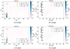 |
Fig. A.1. Same as Figure 4 but for 8123 Keplerian models (153 stable) within the 90% confidence level of χν, best2 as they resulted from optimization Run 2 for dataset A (top) and for 8123 Newtonian models (93 stable, bottom). |
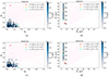 |
Fig. A.2. Same as Figure 4 but for 6055 Keplerian models (198 stable) within the 90% confidence level of χν, best2 as they resulted from optimization Run 1 for dataset B (top) and for 6055 Newtonian models (171 stable, bottom). |
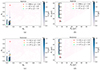 |
Fig. A.3. Same as Figure 4 but for 8216 Keplerian models (454 stable) within the 90% confidence level of χν, best2 as they resulted from optimization Run 2 for dataset B (top) and for 8216 Newtonian models (423 stable, bottom). |
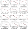 |
Fig. A.4. Newtonian fits for both datasets [A: (a)-(f), B: (g)-(l)] and optimization runs [1: (a)-(c), (g)-(i), 2: (d)-(f), (j)-(l)]. The best-fitting curves (χν, best2) result to dynamically unstable configurations, while the fitting curves of the minimum and maximum reduced chi-square value (χν, min2, χν, max2) define the χν2 limits among all stable configurations. The parameters of each case can be found in Table 4 and Table 5. |
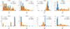 |
Fig. A.5. Histograms resulted from optimization runs. Top: Normalized histograms of eb, ec, Pb, Pc for the Keplerian models as they resulted from the optimization Run 1 for both datasets A, B. The dashed lines indicate the center value of the bin with the maximum frequency. Bottom: Same as top panel but for optimization Run 2. |
Appendix B: Times of minima of NSVS 14256825
Times of minima (1999-2024) of NSVS 14256825 (literature and new).
Times of minima (1999-2024) of NSVS 14256825 (literature and new).
All Tables
Grid search optimization results of Keplerian two-planet LTTE fit after Run 1 of the fitting process for both datasets (A and B).
Grid search optimization results of Keplerian two-planet LTTE fit after Run 2 of the fitting process for both datasets (A and B).
Self-consistent Newtonian two-planet orbital fits initialized from the results of optimization Run 1 for both datasets (A and B).
Self-consistent Newtonian two-planet orbital fits initialized from the results of optimization Run 2 for both datasets (A and B).
All Figures
|
Fig. 1. (a) TESS LC time series composed of three segments (sector 51), (b) phase-folded binned LCs for each segment. |
| In the text | |
|
Fig. 2. ETV diagrams of NSVS 14256825. (a) ETV diagram of dataset A spanning 26 years (1999–2024). Archival data ∼black open circles; NSVS+ASAS data ∼blue open circles; Mythodea data ∼orange open circles; TESS data ∼green open circles; B.R.N.O. data ∼red open circles. (b) ETV diagram of dataset B spanning 18 years (2007–2024). Color indexing is the same as in (a). |
| In the text | |
|
Fig. 3. Differences of the LTTE signals derived from a typical Jacobian fit and from respective osculating N-body models integrated numerically with the inferred initial condition at the osculating epoch T0 = 54274.20875 BJD of the zeroth cycle, where the two models seem to agree. |
| In the text | |
|
Fig. 4. Top: Lifetime colormap plots in the (a) eb, ec and (b) Pb, Pc planes for 5838 Keplerian models (99 stable) within the 90% confidence level of χν, best2 as they resulted from optimization Run 1 for dataset A. Bottom: Same as top but for 5838 Newtonian models (74 stable). The color coding displays the range of lifetimes from white to dark blue, while the orange and green crosses correspond to the positions of the minimum- and maximum-reduced chi-square value of the stable configurations. The best-fitting curve to the data is identified by the red cross, which is unstable in all cases. The MMR solutions have been labeled in the Pb, Pc plane for the nominal Pb = 7 yr. |
| In the text | |
|
Fig. 5. Keplerian fits for both datasets [A: (a)–(f), B: (g)–(l)] and optimization runs [1: (a)–(c), (g)–(i), 2: (d)–(f), (j)–(l)]. The best-fitting curves (χν, best2) result in dynamically unstable configurations, while the fitting curves of the minimum- and maximum-reduced chi-square value (χν, min2, χν, max2) define the χν2 limits among all stable configurations. The parameters of each case can be found in Tables 2 and 3. |
| In the text | |
|
Fig. 6. ETV diagrams with synthetic curves. Left: Keplerian fit of two-planet Jacobian solution (Table 2, χν, min2, dataset A). Right: N-body synthetic curve for the osculating initial condition derived through the formal transformation of the Jacobian elements (Keplerian fit) to the N-body Cartesian osculating frame, centered at the CM of the binary. |
| In the text | |
|
Fig. 7. Orbital evolution of (a) eccentricities and (b) semi-major axes for the inner and outer planets over 100 Myr (dataset B, Run 1, χν, min2). (c) The temporal variation of the χν, min2 fitting curve (dataset B, Run 1) over the first 152 years is represented by five sets of parameters, each corresponding to a complete outer orbit revolution (38 years). The black synthetic curve is the Keplerian (kinematic) fit from which this dynamical model was initialized, and it appears to be in absolute agreement with the first 38 years of orbital evolution (green curve) and in close agreement with the subsequent fits (blue and red curves). |
| In the text | |
|
Fig. 8. Temporal evolution of resonant angles (a) θ1, (b) θ2, and (c) θ3 of a stable solution close to the 3:1 MMR (Table 2, χν, min2, dataset A) over the first 10 000 years of integration. |
| In the text | |
|
Fig. A.1. Same as Figure 4 but for 8123 Keplerian models (153 stable) within the 90% confidence level of χν, best2 as they resulted from optimization Run 2 for dataset A (top) and for 8123 Newtonian models (93 stable, bottom). |
| In the text | |
|
Fig. A.2. Same as Figure 4 but for 6055 Keplerian models (198 stable) within the 90% confidence level of χν, best2 as they resulted from optimization Run 1 for dataset B (top) and for 6055 Newtonian models (171 stable, bottom). |
| In the text | |
|
Fig. A.3. Same as Figure 4 but for 8216 Keplerian models (454 stable) within the 90% confidence level of χν, best2 as they resulted from optimization Run 2 for dataset B (top) and for 8216 Newtonian models (423 stable, bottom). |
| In the text | |
|
Fig. A.4. Newtonian fits for both datasets [A: (a)-(f), B: (g)-(l)] and optimization runs [1: (a)-(c), (g)-(i), 2: (d)-(f), (j)-(l)]. The best-fitting curves (χν, best2) result to dynamically unstable configurations, while the fitting curves of the minimum and maximum reduced chi-square value (χν, min2, χν, max2) define the χν2 limits among all stable configurations. The parameters of each case can be found in Table 4 and Table 5. |
| In the text | |
|
Fig. A.5. Histograms resulted from optimization runs. Top: Normalized histograms of eb, ec, Pb, Pc for the Keplerian models as they resulted from the optimization Run 1 for both datasets A, B. The dashed lines indicate the center value of the bin with the maximum frequency. Bottom: Same as top panel but for optimization Run 2. |
| In the text | |
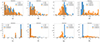 |
Fig. A.6. Same as Figure A.5 but for the Newtonian models. |
| In the text | |
Current usage metrics show cumulative count of Article Views (full-text article views including HTML views, PDF and ePub downloads, according to the available data) and Abstracts Views on Vision4Press platform.
Data correspond to usage on the plateform after 2015. The current usage metrics is available 48-96 hours after online publication and is updated daily on week days.
Initial download of the metrics may take a while.