| Issue |
A&A
Volume 691, November 2024
|
|
|---|---|---|
| Article Number | A207 | |
| Number of page(s) | 11 | |
| Section | Stellar atmospheres | |
| DOI | https://doi.org/10.1051/0004-6361/202450105 | |
| Published online | 13 November 2024 | |
Optimised use of interferometry, spectroscopy, and stellar atmosphere models for determining the fundamental parameters of stars
1
Université Côte d’Azur, Observatoire de la Côte d’Azur, CNRS, Laboratoire Lagrange,
France
2
Max Plank Institute for Astronomy,
69117
Heidelberg,
Germany
3
Niels Bohr International Academy, NBI, University of Copenhagen,
Blegdamsvej 17,
2100
Copenhagen,
Denmark
4
Space Sciences, Technologies and Astrophysics Research (STAR) Institute, Université de Liège,
Quartier Agora, Allée du 6 Août 19c, Bât. B5C,
4000
Liège,
Belgium
5
Instituto de Astrofísica de Andalucía (IAA-CSIC),
Glorieta de la Astronomía s/n,
18008
Granada,
Spain
6
INAF- Palermo Astronomical Observatory, Piazza del Parlamento, 1,
90134
Palermo,
Italy
7
LUPM, Univ Montpellier, CNRS,
Montpellier,
France
8
Institut de Recherche en Astrophysique et Planétologie, Université de Toulouse, CNRS,
IRAP/UMR 5277, 14 Avenue Édouard Belin,
31400
Toulouse,
France
★ Corresponding author; This email address is being protected from spambots. You need JavaScript enabled to view it.
Received:
23
March
2024
Accepted:
27
September
2024
Abstract
Context. Thanks to recent progress in the field of optical interferometry, instrument sensitivities have now reached the level achieved in the domain of new space missions dedicated to exoplanet and stellar studies. Combining interferometry with other observational approaches enables the determination of stellar parameters and helps improve our understanding of stellar physics.
Aims. In this paper, we aim to demonstrate a new way of using stellar atmosphere models for a joint interpretation of spectroscopic and interferometric observations.
Methods. Starting from a discrete grid of one-dimensional (1D) stellar atmosphere models, we developed a training algorithm, based on an artificial neural network, capable of estimating the spectrum and intensity profile of a star over a range of wavelengths and viewing angles. A minimisation algorithm based on the trained function allowed for the simultaneous fitting of the observational spectrum and interferometric complex visibilities. As a result, coherent and precise stellar parameters can be extracted.
Results. We show the ability of the trained function to match the modelled intensity profiles of stars in the effective temperature range of 4500–7000 K and surface gravity range of 3 to 5 dex, with a relative precision to the model that is better than 0.05%. Using simulated interferometric data and actual spectroscopic measurements, we demonstrated the performance of our algorithm on a sample of five benchmark stars. Using this method, we achieved an accuracy within 0.5% for the angular diameter, radius, and surface gravity, and within 20 K for the effective temperature.
Conclusions. This paper demonstrates a new method of using interferometric data combined with spectroscopic observations. This approach offers an improved determination of the radius, effective temperature, and surface gravity of stars.
Key words: instrumentation: interferometers / stars: fundamental parameters
© The Authors 2024
 Open Access article, published by EDP Sciences, under the terms of the Creative Commons Attribution License (https://creativecommons.org/licenses/by/4.0), which permits unrestricted use, distribution, and reproduction in any medium, provided the original work is properly cited.
This article is published in open access under the Subscribe to Open model. This email address is being protected from spambots. You need JavaScript enabled to view it. to support open access publication.
1 Introduction
In the field of modern optical interferometry, there is a longstanding interest in studying the fundamental parameters of stars. Numerous studies have been conducted over the years with the aim of developing analytical descriptions of the stellar intensity profiles for a reliable estimation of the angular diameter. Some notable studies in this area include the works of Hanbury Brown et al. (1974); Diaz-Cordoves & Gimenez (1992); Claret (2000); Davis et al. (2000) and Claret & Southworth (2022). A pragmatic approach is to numerically calculate the wavelength-dependent intensities at given locations on the stellar disk, commonly described by the parameter µ = cos α, where α is the angle between the observer’s line of sight and the surface normal (Claret 2000; Claret & Southworth 2022). The intensity profiles are often approximated by a limb-darkening (LD) law with a small number of coefficients (Claret 2000; Espinoza & Jordán 2016; Morello et al. 2020).
In recent years, it has been recognised that having an accurate description of the intensity profile is crucial for the interpretation of transit light curves. In the past, various works such as those of Hanbury Brown et al. (1974); Claret (2000); Kervella et al. (2017), have utilised stellar atmosphere models to either predict LD coefficients or interpret interferometric measurements. Kervella et al. (2017) compared various LD laws from different stellar atmosphere models with observations and found that the square root law or a four-parameter law provided the best fit, even though they were not significantly more accurate than the single-parameter power law.
The key astrophysical objectives of the CHARA/SPICA1 instrument (Mourard et al. 2022) include the completion of a large and homogeneous survey of fundamental stellar parameters, based on about one thousand stellar angular diameter measurements. Thanks to a reachable angular resolution down to 0.2 mas with this instrument, we have the ability to observe a few hundred dwarf stars. This will enable direct angular diameter and LD measurements for a wide range of effective temperature and surface gravity. This objective is complementary to the need to reach a precision of a few per cent for the stellar radius of the core programme PLAnetary Transits and Oscillations of stars (PLATO) mission targets (Rauer et al. 2024).
In this paper, we propose and demonstrate a new way of analyzing the interferometric data by combining them with spectroscopic data, photometric data, and 1D stellar atmosphere models. This method is intended to permit direct estimations of the stellar angular diameter (θ), simultaneously with a precise estimation of the effective temperature (Teff) and of the surface gravity (log g). In addition, we can combine the measured angular diameter with the stellar parallax to get the physical radius of the star. The first step is to use a grid of intensity profiles calculated using stellar atmosphere models and detailed nonlocal thermodynamic equillibrium (NLTE) radiative transfer in the post-processing over a representative range of Teff and log g, leaving the other parameters fixed. This grid is used to train a machine learning (ML) algorithm for being able to compute the intensity profiles of any star in a predefined range of parameters and incidence angles assumed in the grid. This continuous function is then used in a model-fitting process to match interferometric data and estimate the angular diameter, Teff, and log g values. Finally, this process is combined with a similar algorithm based on the same initial grid and aimed at including spectroscopic data as well.
In Sect. 2, we describe the grid of Model Atmospheres with a Radiative and Convective Scheme (MARCS) atmosphere models used and the application of our ML process to this grid. Then in Sect. 3, we briefly present the standard interferometric method based on simple geometric model of the LD and we detail our new method based on the MARCS grid and the ML process. In Sect. 3.4, we present the complete modelling of the interferometric, spectroscopic and photometric data to improve the determination of stellar parameters, including Teff and log g. We present a discussion in Sect. 4 and our conclusion in Sect. 5.
2 Theoretical intensity profiles
2.1 The initial grid
We use MARCS model atmospheres (Gustafsson et al. 2008), which were computed under assumptions of 1D hydrostatic equilibrium and local thermodynamic equilibrium (LTE). Disk-resolved synthetic spectra were computed using the NLTE version of the spectrum synthesis code Turbospectrum (TS, Plez 2012; Gerber et al. 2023). The wavelength range of the grid is 400 to 900 nm and the spectral resolving power is set to R = 200 000. Our TS grid was first used by Morello et al. (2022) for computing stellar LD tables. To match the core of the PLATO mission, the stellar parameter space covered by the grid of synthetic stellar spectra is two dimensional, with Teff between 4500 and 7000 K, and log g between 3 and 5 dex, with a random sampling of 200 models from the original MARCS grid of Gustafsson et al. (2008), as represented in Fig. 1. As in Gerber et al. (2023), for spectrum syntheses with TS, we use the solar abundances from Magg et al. (2022), which were carefully determined using state-of-the-art atomic and molecular data, NLTE model atoms, opacities, and new high-quality solar observations with TS-NLTE. This is done to ensure maximal consistency in the spectroscopy module of the pipeline and in all other modules in the Stellar Abundances and atmospheric Parameters Pipelines (SAPP, Gent et al. (2022)) that make use of TS-NLTE synthetic grids (see Sect. 3.4 for more details). To accelerate our calculations and to adapt them to the interferometric data of CHARA/SPICA, we then degraded the resolving power from R = 200 000 down to a resolution of about 140, sampling 59 spectral channels between 600 and 900 nm.
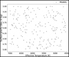 |
Fig. 1 Random samples of 200 models taken from the MARCS grid as a function of effective temperature and surface gravity. |
2.2 Radau sampling
The MARCS spectral intensity profiles were evaluated at 12 µ values following the Radau sampling, with  , where α is the angle between the normal to the surface and the line of sight and ρ is the normalised radius. This non-homogeneous sampling nicely captures the rapid change in intensity near the edge and ensures the precise computation of interferometric observables with fewer points than other samplings.
Minimising the number of µ values helps to reduce the computing time when producing and using a large grid of intensity profiles. The Radau values of µ are given by the roots of a combination of Legendre polynomials, Pn :
 (1)
(1)
where µ ranges from 1 to 0, while x ranges from −1 to 1. The µ1 = 1 (x1 = −1) value is always present in the sampling. Figure 2 shows the Radau-sampling values of µ as computed using Eq. (1).
Centre-to-limb variations are known to be very smooth in 1D models, and using 12 points is generally sufficient to describe the intensity variation at all wavelengths, λ. According to Morello et al. (2022), the 12 sampling rate is adequate for the intensity profile computations in transit analysis of exoplanets. Further increasing the sampling rate is unnecessary, as the limitations of the models will then become more prominent. As shown in Fig. 3, compared to different two-coefficient LD laws, the square root law provides the closest match to the intensity profiles from MARCS. It strongly outperforms the most popular quadratic law (Kopal 1950) and is comparable to the power 2 law (Hestroffer 1997), in line with recent tests on exoplanetary transits (Morello et al. 2017; Maxted 2018).
To confirm that a sampling with 12 points is also sufficient for the interferometric observations, we compared the square visibility obtained using the analytical equation of the square root law (chosen for this test) and the square visibility obtained by performing the Hankel transform (HT) of a 1D intensity profile using the Radau quadrature (with 12 points).
Domiciano de Souza et al. (2021) present the analytical complex visibility relation obtained using the HT from a general polynomial form of the intensity profile. The intensity profile for the square root LD law is given by:
 (2)
(2)
where c and d are the coefficients of square-root law, I(µ) is the intensity and I(1) is the maximum intensity.
Computing the HT for the square-root LD law results in the following complex visibility equation:
 (3)
(3)
where Γ is the gamma function, Jν(z) is the Bessel function of the order of ν. The dimensionless variable z is given by πθB/ λ, where B is the interferometric baseline length projected onto the viewing direction, λ is the wavelength, and θ is the angular diameter.
Figure 4 shows the comparison between the analytical expression of the visibility and the computation through the HT method and the Radau sampling. We can conclude that up, to z ≃ 20, the agreement of the 12 Radau sampling is almost perfect. With the longest baseline of CHARA (B=330 m), the mean wavelength of SPICA (λ = 750 nm), this condition is respected for angular diameters θ smaller than 3 mas. For the larger stars, an increase in the number of points for the Radau sampling or a limitation of the maximum baseline will be necessary.
From these results, we can conclude that the 12 Radau sampling, as proposed by Morello et al. (2022) for the study of transits, is also in line with the current highest spatial resolution permitted by long baseline interferometry in the visible up to θ of 3 mas. The corresponding range on θ of stars can be estimated, for example, using the surface brightness colour relation (SBCR) from Salsi et al. (2020), for dwarfs ((V-K) from 1 to 3, covering the PLATO range):
 (4)
(4)
From Eq. (4), we may conclude that the interferometric observations with CHARA/SPICA of all F5-K7 dwarf stars fainter than magnitude, V = 4.3, could be correctly interpreted by this 12 Radau sampling without introducing any systematics. Similar calculations could be done of course for other spectral types or luminosity classes using other SBCR relations.
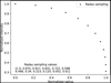 |
Fig. 2 Radau-sampling on the normalised intensity profile along the normalised radius of a star with Teff = 6100 K and log g = 3.79 dex at λ = 725 nm. The 12 µ values, listed inside the figure, are computed usin Eq. (1). The values are iven from the centre of the star (radius = 0) to the limb (radius=1). |
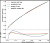 |
Fig. 3 Comparison of different LD laws to the intensity profile from MARCS model at Teff = 5022 K and log g = 3.76 dex (top). The difference between MARCS model and each LD law (bottom). |
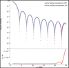 |
Fig. 4 Square visibility of a star obtained using the analytical square root law (A, blue) and (orange) with a Hankel Transform (HT), with Radau quadrature for 12 µ values, plotted as a function of z = πθB/λ, where θ is in radian, and B and λ in meter (top). The difference between the square visibility of the star computed with these two methods (bottom). |
2.3 Machine learning for intensity profiles
Since the MARCS grid is a set of discrete stellar atmosphere models, we used a fast reconstruction technique based on artificial neural networks (ANN) to recover the intensity profile as a function of λ for 12 different µ values at any given Teff and log g. The idea is to train a set of ANNs with the intensity profile grid (described in the previous section) and to reconstruct the intensities using these networks. We performed this with the Pytorch (Paszke et al. 2019) ML library in Python.
Supervised learning on the data was implemented, where inputs (Teff and log g of the star) and corresponding results (intensity profile as a function of wavelength λ and viewing angle µ) were given to the ANN during the training process. The ML process was executed with a multi-layered ANN using a combination of five linear layers and rectified linear units (ReLU), which acts as the activation function. A five-layer network was ideal for capturing the pattern of a data set with three parameters (intensity, wavelength, µ), giving an improved model performance in terms of accuracy and generalisation. The architecture of the ANN is designed with a similar concept as the neural network in Kovalev et al. (2019).
To make the learning process simple and efficient, the data were subdivided into smaller batches and divided into three groups: training, evaluation, and test sets. Overall, 85% of the samples was allocated to the training set, 10% to the evaluation set, and 5% to the test set. This ensures that there are enough data used to train the ANN, evaluate and validate its performance (make necessary changes if required) and test its efficiency on the set of data not involved in training the ANN. Keeping this in three separate sets ensures that different data are used at various steps and this can also avoid bias during the testing of the output intensity. The initial learning rate in the network was set at 10−5 . The small learning rate allows the network to learn the training set with high accuracy. At each epoch (loop for training the network), the training of ANN with binned data and the training loss (between the true value and reconstructed output) were calculated. At the same iteration, after the training, an evaluation of the training and its losses was also performed. The loss at each step is quantified using the mean squared error loss (MSE) and the optimisation of the training was performed using an adaptive moment estimation (ADAM) optimiser, which is a combination of a stochastic gradient descent (SGD) optimisation and the root mean squared propagation in Pytorch (Paszke et al. 2019). The optimisation is aimed at setting the weights, bias, and learning rate according to the loss calculated to reduce it. It improves the efficiency and the accuracy of the ANN reconstructions. The training is continued until the loss in evaluation is less than 0.001. Once we have the weights and bias of the ML with this least loss, it can be saved and used in reconstructing any intensity profiles in the given range of input parameters Teff and log g.
Figure 5 (top) shows the intensity profiles from one sample taken from the MARCS model (red) overplotted with the intensity profiles reconstructed using the ANN (blue) with the same Teff and log g randomly chosen from the test set, as a function of λ and for different µ angles. The reconstructed values match the initial intensity profiles with a relative error around 10−3 to 10−4, as seen from the Fig. 5 (bottom). Multiple tests were carried out at random positions in the initial Teff and log g grid, each giving consistent results.
3 Improved application of interferometric data
3.1 Simulating observation
Since CHARA/SPICA is still in its early phase of operation, the test of our new pipeline was based on simulated interferometric data. We considered the five Gaia benchmarks (Heiter et al. 2015) listed in Table 1.
As stated by the Van Cittert-Zernike theorem, the interferometric observables can be obtained by computing the Fourier transform of the source brightness distribution. Considering the spherical symmetry of the stellar surface in the cases considered here, we can use the HT (Hestroffer 1997; Domiciano de Souza et al. 2021) which is much faster in terms of computational time than a two-dimensional (2D) Fourier transform. This is particularly true if a Radau quadrature method with only a dozen of points is used, as in our case.
The method for the computation of the simulated data is presented in Fig. 6. We used an interferometric observation preparation tool called Aspro22. It generates actual UV coordinates and spectral bands for CHARA/SPICA and allows for the spatial frequencies used later in the HT computation to be calculated.
The intensity profile of the benchmark stars, for the given Teff and log g, can be obtained with the ANN-trained MARCS grid. Combining the spatial frequencies, intensity profile, and angular diameter, we can obtain the square visibility through the HT computation. However, this visibility does not include any noise or bias that occurs during an observation. To mimic the noise while observing, we set a signal-to-noise ratio (S/N) of 20 on the square visibility. Based on this estimation of statistical noise, we build a Gaussian distribution of 3σ and we randomly obtained an additional term added to the computed visibility as a bias. By using this method, we can generate a representative sample of square visibility for the 15 baselines and the 59 different spectral channels that are expected for the CHARA/SPICA observations. The obtained square visibility is saved as an OIFits file (see Duvert et al. 2017), akin to an actual observation.
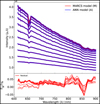 |
Fig. 5 Intensity from the MARCS model (red) as a function of λ for 12 different µ values (Radau sampling) along the radius over-plotted on the reconstructed values from the ANN (blue and thicker) for the same Teff and log g (top). From top to bottom, the figure presents the intensity profiles in ascending order of radius (or descending order of µ). The intensity profile of the model at Teff = 6176 K and log g = 3.82 dex is also given (bottom). This plot represents (in terms of percentage) the residual between the intensity from MARCS and the intensity values from the ANN for the different µ values. |
Comparison of stellar parameters using different methods.
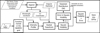 |
Fig. 6 Flow chart giving the steps to simulate the interferometric data mimicking CHARA/SPICA observations. The pipeline carries out a Hankel transform on the intensity profile from the stellar radiation transfer calculations, using the UV coordinates and wavelength from Aspro2. The error is added to the square visibility, taking S/N = 20 and generates an error with a random extraction for each point in the square visibility. Input and output are shown in parallogram (grey) and intermediate processes are shown in rectangle (black). |
3.2 The classical method for interferometry
To evaluate our new pipeline, we briefly report on the classical way interferometric data are used up to now. We call this the classical method for interferometry. We use LITpro3, an interferometric model fitting tool to estimate the angular diameter on the simulated data. In LITpro, we used a square root LD law.
For all the benchmark stars, with the exception of 18 Sco, the LD coefficients are also fitted simultaneously to the angular diameter. In the case of 18 Sco, which exhibits a small angular diameter (less than 0.8 mas), the data are not very sensitive to the LD profile. In that case, we set the coefficients using the Claret table (Claret & Bloemen 2011). However, this method carries the disadvantage of underestimating the error on the angular diameter. Consequently, for stars with small apparent size, such as 18 Sco, the relative error on the angular diameter was adjusted to be 1% to solve this limitation.
We used the parallax (πp ) in arcsecond from the Gaia DR3 when available otherwise (η Boo, Procyon) from HIPPARCOS (van Leeuwen 2007). The radius (in solar radius, R⊙) is then estimated following:
 (5)
(5)
The constant term is based on the most recent solar constants (Prša et al. 2016). Simultaneously, the effective temperature is calculated using the bolometric flux (fbol, in erg s−1 cm−2) from the photometric module of the SAPP (Gent et al. 2022), and the angular diameter:
 (6)
(6)
where C is the conversion from parsec to centimetre (3.086 × 10¹⁸), σ stands for the Stefan-Boltzmann constant (5.67 × 10⁻⁵ erg cm−2 s−1 K−4), and the solar radius (R⊙) is taken in centimetres. The errors associated with the estimated radius and effective temperature are determined using the standard error propagation.
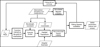 |
Fig. 7 Flow chart illustrating the fitting method for interferometry. Input and output are shown in parallogram (grey) and intermediate processes are shown in rectangle (black). |
3.3 Using the grid and the ML for the interferometric data
In this subsection, we present the direct fitting of the interferometric data on the grid and the ML function, referred to as the ‘interferometry alone’ method below. The flow chart of this method is shown in Fig. 7. The pipeline takes the interferometric data as input. Using the trained ANN described in Sect. 2.3, we can get the intensity profile of any FGK stars. To initiate the fitting, an intensity profile with Teff and log g close to that of the observation is taken, and the angular diameter is set to an arbitrary initial value of 1 mas. Using the UV coordinates from the input data, the square visibility of the model ( ) can be calculated using HT. We performed a quick parameter estimation based on a chi-square (χ2) minimisation on the square visibility (V2) using scipy.optimize function in Python and keeping the angular diameter, Teff, and log g as free parameters. Then, starting from this first estimation, the model fitting was done using a Markov chain Monte Carlo (MCMC) sampler using emcee (Foreman-Mackey et al. 2013) to sample the posterior probability distribution of these parameters. Measurement values (e.g. median) and uncertainties for the free parameters were then extracted from these posteriors distributions. For stars with an apparent size greater than 3 mas, we cut the interferometric data at spatial frequencies corresponding to z = 20 before the model fitting, as explained in Sect. 2.2.
The results of this method for the five benchmark stars are presented in Table 1 in ‘ML method for interferometry alone’. If the method presented here may seem better as it uses stellar atmosphere models instead of an analytical description of LD, it turns out that the diameters are correctly recovered but the interferometric data alone are not enough to reach reliable and accurate information on Teff and log g. Indeed, interferometry is only sensitive to the intensity profile of the stars and (considering the current accuracy and spatial frequency sampling) it is not possible to distinguish subtle changes of profiles when changing the temperature or the surface gravity.
3.4 Combining interferometry, spectroscopy, and photometry
As shown from the results in Sect. 3.3, using interferometry alone is not efficient in terms of estimating the stellar parameters besides the angular diameter. To achieve a more accurate estimation of the stellar parameters, we combined the interferometric module in Sect. 3.3 with the spectroscopic and photometric modules from the SAPP pipeline as shown in Fig. 8, referred to as the spectroscopic–photometric–interferometric (SPI) method, henceforth. In the pipeline, we used the spectroscopic module (red box in Fig. 8) and the photometric module (green box in Fig. 8) to guide the interferometric module from Sect. 3.3 (brown box in Fig. 8). Using the results from the spectroscopic and photometric module, we can limit the number of the models used in fitting the interferometric module, helping in getting an accurate estimation on Teff and log g.
The SAPP pipeline (Gent et al. 2022), which will be used as a part of the PLATO pipeline, uses a method of model fitting with the spectra to obtain the parameters of the star using a neural network. The current grid is trained with the flux of stellar spectrum from 1D MFAGS-OS NLTE (1D hydrostatic model atmospheres with opacity sampling (OS) Grupp 2004a,b) stellar atmosphere with individual stellar parameters in an 8D grid (Kovalev et al. 2019; Gent et al. 2022). The grid includes parameters Teff, log g, micro-turbulence, and line-broadening (combining macro turbulence and projected rotation velocity), as well as [Fe/H], [Mg/Fe], [Ti/Fe], and [Mn/Fe].
The module for spectroscopy in the SAPP uses a modelfitting method, relying on the gradient descent method, which is an iterative optimisation algorithm that can locate the global minimum in parameter space. The implementation of spectroscopy is shown in the red box of Fig. 8. The observed and synthetic spectra are fitted using χ2 minimisation and yield all spectroscopic quantities, including Teff, metallicity, and other quantities used in training the grid. In this paper, we show the results for five Gaia benchmark stars (Table 1) and for them, we use the optical GIRAFFE HR10 (High Resolution) spectra obtained within the Gaia-ESO survey4 (Randich et al. 2022).
To carry out the photometric analysis, we use synthetic photometry, a method similar to that given by Gent et al. (2022). The flow chart of the photometric module is shown in the green box of Fig. 8. This takes the effective temperature (Teff), surface gravity (log g), metallicity, and angular diameter as the input and runs a stellar evolution track (as described in Gent et al. 2022) to get the prior probability of the star parameters. The effective temperature, surface gravity, and metallicity are taken from the spectroscopy, while the angular diameter comes from the initial interferometric run. In the second step, we use the apparent magnitude and extinction5 for bands B, V, J, H, Ks, G, GBP , and GRP from Johnson-Cousins, 2MASS, and Gaia DR3 to calculate the absolute magnitude of the star. Using different bands of photometry helps to increase the accuracy of the calculated magnitude value. In the third part of the module, the absolute magnitude and prior probability are used to estimate the luminosity of the star, along with the photometric surface gravity. By combining the luminosity with the distance of the star, we can obtain the bolometric flux ( fbol), using:
 (7)
(7)
where L⋆ is the luminosity of the star.
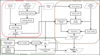 |
Fig. 8 Flow chart representing the pipeline and its different modules combined to get the stellar parameters (brown). Interferometric module (red) Spectroscopic module and (green) Photometric module. Input and output are shown in parallogram (grey) and intermediate processes are shown in rectangle (black). |
4 Discussion
4.1 Comparison of model fitting for interferometry and SPI method
Table 1 shows the values of the stellar parameters estimated using the classical method for interferometry, the ML method for interferometry alone, and the SPI method. The comparison of the different methods applied on the benchmark stars is illustrated in Fig. 9. For the classical method, we calculated the values as explained in Sect. 3.2. However, it should be noted that the uncertainty on Teff tends to be underestimated, as explained in Gent et al. (2022). Values for the interferometry alone method and SPI methods were estimated according to the procedure described in Sects. 3.3 and 3.4.
From the angular diameter plot, we see that all the methods are efficient in correctly determining the value within the error bars, but the SPI method gives the most reliable one. However, interferometry alone is not sufficient to accurately estimate other fundamental parameters such as Teff and log g, as seen in the two upper plots of Fig. 9. When attempting to estimate these parameters using the interferometry alone method, it was noticed that multiple intensity profiles could be fitted within a small range of Teff and log g, resulting in a high error of up to 1700 K in some cases (Procyon, as seen in Table 1).
Clearly, the SPI method succeeds in recovering correctly the initial parameters and provides an average accuracy of about 20 K on effective temperature. For the angular diameter, radius, and (in particular) for log g, the accuracy achieved with the SPI method is also better than for the other methods, achieving a relative accuracy of less than 0.5%. Figure 10 shows the corner plots for β Vir obtained with the MCMC sampling for the interferometry alone and SPI methods. For the SPI method, it is clear that the shape of the different distributions of probability does not exhibit any correlations between parameters, except of course between the radius and the angular diameter. As expected, the combination of the different datasets greatly improves the reliability of the estimation of the parameters. The corner plots for the SPI method are given for the four other benchmark stars in Appendix A.
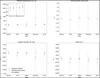 |
Fig. 9 Plot comparing the difference of the input values (I) and values of parameters from different methods (E) in the Table 1. Top-left: effective temperature (Teff), with a zoom between −200 to 150 K, (top right) surface gravity (log g), (bottom-left) angular diameter (θ), and (bottom-right) radius. |
4.2 Impact of metallicity
In the model grid used in the interferometric module of the pipeline, the assumption is that stars have solar abundance. For stars with a metallicity differing within ±0.5 dex from solar metallicity, the differences in intensity profile do not change the estimate of the stellar parameters. However, for stars with a larger metallicity difference, the impact on the LD of the star is much greater, as seen in Fig. 11. When the metallicity was altered to ±1 dex solar metallicity, while keeping all other parameters constant, it was observed that there can be up to a 15% change in the intensity profile. This could lead to larger errors in the estimation of the stellar parameters.
In the work presented here, the impact of metallicity can be overlooked, as that of all the benchmark stars lies within 0.5 dex of the solar value.
In the future, we plan to include metallicity as the fourth parameter in the grid for ML. This will allow us to extend the use cases of our method without degrading the accuracy of the fundamental parameter estimations. Additionally, the grid will be expanded to include the H and K bands on the interferometric observation, such as Michigan InfraRed Combiner-eXeter (MIRCX, Anugu et al. 2020) and Michigan Young STar Imager at CHARA (MYSTIC, Monnier et al. 2018) instruments at CHARA. Including the H and K bands along with the R band from CHARA/SPICA observations will provide more constrain to the square visibility fitting and will increase the reliability of the pipeline.
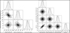 |
Fig. 10 Parameter range for β Vir (corner plot). The solid line in the plot is the median value after running MCMC, the dotted line represents 1σ and the contours on the plot represent 1, 2, and 3σ. The corner plot for interferometry alone (left) and the combined corner plots (right) with interferometry, spectroscopy, and photometry (SPI method). |
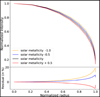 |
Fig. 11 Comparison of intensity profile for Teff = 5750 and log g = 4.00 dex showing the sensitivity of LD to metallicity. (top) The analytical intensity profile was plotted using the square-root law. The residual between the intensity profiles at different metallicity with respect to the solar value (bottom). |
4.3 Applications
The method presented here will be used for the Interferometric Survey for Stellar Parameter (ISSP) (Mourard et al. 2022; Ligi et al. 2023). The survey aims to observe about a thousand stars using a consistent dataset and analysis method over the next three years, employing the CHARA/SPICA instrument. The survey’s primary goal is to obtain angular diameter values with a precision of 1% and other fundamental parameters with precision of 2%. The method showcased in this work will be used to obtain these parameters and create a catalogue of stars with high-precision fundamental values.
In addition, the pipeline will mainly be used in the context of PLATO for two closely related purposes. First, we aim to improve our knowledge of the benchmark stars for the mission to ensure that the (seismic) methods used to determine the stellar radii of the solar-like, core programme targets are well calibrated. Indeed, there are many targets in common between the ISSP survey and PLATO. Second, we aim to accurately measure the radius of the stars hosting transiting planets to be discovered by this mission, so that the planetary radius is tightly constrained as well.
5 Conclusion
In this work, we have proposed a new and innovative method to estimate the angular diameter and other stellar parameters of FGK-type dwarf stars. Our approach employs an ANN and integrates multiple observations, including interferometry, spectroscopy, and photometry. With the high precision of the ANN making it adept at reconstructing the intensity profile, the SPI method helps to achieve a high accuracy in terms of estimating the parameters. Compared to other applied methods, SPI has a significantly improved accuracy when estimating stellar parameters – and with smaller errors.
We tested the pipeline on a sample of FGK-type Gaia benchmark stars. To test it, we simulated interferometric observations as observed using CHARA/SPICA and spectroscopic observation from the Gaia-ESO Survey. Our pipeline can recover the parameters with an accuracy of less than 0.5% for the θ, radius, and log g, and less than 20 K for Teff, as shown in Table 1.
As already highlighted in Gent et al. (2022), the scientific approach we have developed in this paper will be integrated in the SAPP pipeline, and other components of the PLATO analysis pipelines. In the future, we are planning to use three dimension (3D) NLTE grids of synthetic stellar spectra computed using 3D radiation-hydrodynamics simulations of stellar atmospheres, such as the STAGGER (Nordlund 1982; Nordlund & Galsgaard 1995; Collet et al. 2011), MURaM (Vögler et al. 2004, 2005), CO5BOLD (Freytag et al. (2012)), and Dispatch (Nordlund et al. 2018; Eitner et al. 2024). Alternatively, 1D hydrostatic models with tailored parameterisation of convection and/or sphericity can be implemented to improve the efficiency of calculations (e.g. Kostogryz & Berdyugina 2015; Kostogryz et al. 2016, 2022). This may help to substantially improve the accuracy of astrophysical parameters derived from interferometric constraints, as demonstrated from studies of centre-to-limb variation of stars (e.g. Pereira 2009; Beeck et al. 2012; Hayek et al. 2012; Pereira et al. 2013; Ludwig et al. 2023; Witzke et al. 2024). Nordlund et al. (2009) has provided an extended discussion of the centre-to-limb variation in 3D radiation magnetohydrodynamics simulations. In addition, it is worth noting that this work can be easily extended to other spectral types and luminosity classes by training the ANN with adequate model grids.
Acknowledgements
This project has received funding from the European Research Council (ERC) under the European Union’s Horizon 2020 research and innovation programme (Grant agreement No. 101019653). T.M. acknowledges financial support from Belspo for contract PRODEX “PLATO mission development”. G.M. acknowledges financial support from the Severo Ochoa grant CEX2021-001131-S and from the Ramón y Cajal grant RYC2022-037854- I funded by MCIN/AEI/10.13039/501100011033 and FSE+. This research has made use of the Jean-Marie Mariotti Center Aspro service. B. Plez acknowledges support from the French National Space Agency (CNES).
Appendix A Corner plot presenting the distribution of probability for the different parameters of the model
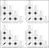 |
Fig. A.1 Corner plots presenting the distributions of probability for the different parameters of the model from the SPI method of 18 Sco (top left), δ Eri (top right), η Boo (bottom left), and Procyon (bottom right). The solid line in the plot is the median value after MCMC and the dotted line represents 1σ. The contours are drawn at 1, 2, and 3σ. |
References
- Anugu, N., Le Bouquin, J.-B., Monnier, J. D., et al. 2020, AJ, 160, 158 [NASA ADS] [CrossRef] [Google Scholar]
- Beeck, B., Collet, R., Steffen, M., et al. 2012, A&A, 539, A121 [NASA ADS] [CrossRef] [EDP Sciences] [Google Scholar]
- Claret, A. 2000, A&A, 363, 1081 [NASA ADS] [Google Scholar]
- Claret, A., & Bloemen, S. 2011, A&A, 529, A75 [NASA ADS] [CrossRef] [EDP Sciences] [Google Scholar]
- Claret, A., & Southworth, J. 2022, A&A, 664, A128 [NASA ADS] [CrossRef] [EDP Sciences] [Google Scholar]
- Collet, R., Magic, Z., & Asplund, M. 2011, in Journal of Physics Conference Series, 328, 012003 [NASA ADS] [CrossRef] [Google Scholar]
- Davis, J., Tango, W. J., & Booth, A. J. 2000, MNRAS, 318, 387 [Google Scholar]
- Diaz-Cordoves, J., & Gimenez, A. 1992, A&A, 259, 227 [Google Scholar]
- Domiciano de Souza, A., Zorec, J., Millour, F., et al. 2021, A&A, 654, A19 [NASA ADS] [CrossRef] [EDP Sciences] [Google Scholar]
- Duvert, G., Young, J., & Hummel, C. A. 2017, A&A, 597, A8 [NASA ADS] [CrossRef] [EDP Sciences] [Google Scholar]
- Eitner, P., Bergemann, M., Hoppe, R., et al. 2024, A&A, 688, A52 [NASA ADS] [CrossRef] [EDP Sciences] [Google Scholar]
- Espinoza, N., & Jordán, A. 2016, MNRAS, 457, 3573 [NASA ADS] [CrossRef] [Google Scholar]
- Foreman-Mackey, D., Hogg, D. W., Lang, D., & Goodman, J. 2013, PASP, 125, 306 [Google Scholar]
- Freytag, B., Steffen, M., Ludwig, H. G., et al. 2012, J. Computat. Phys., 231, 919 [NASA ADS] [CrossRef] [Google Scholar]
- Gent, M. R., Bergemann, M., Serenelli, A., et al. 2022, A&A, 658, A147 [NASA ADS] [CrossRef] [EDP Sciences] [Google Scholar]
- Gerber, J. M., Magg, E., Plez, B., et al. 2023, A&A, 669, A43 [NASA ADS] [CrossRef] [EDP Sciences] [Google Scholar]
- Grupp, F. 2004a, A&A, 420, 289 [NASA ADS] [CrossRef] [EDP Sciences] [Google Scholar]
- Grupp, F. 2004b, A&A, 426, 309 [NASA ADS] [CrossRef] [EDP Sciences] [Google Scholar]
- Gustafsson, B., Edvardsson, B., Eriksson, K., et al. 2008, A&A, 486, 951 [NASA ADS] [CrossRef] [EDP Sciences] [Google Scholar]
- Hanbury Brown, R., Davis, J., Lake, R. J. W., & Thompson, R. J. 1974, MNRAS, 167, 475 [NASA ADS] [CrossRef] [Google Scholar]
- Hayek, W., Sing, D., Pont, F., & Asplund, M. 2012, A&A, 539, A102 [NASA ADS] [CrossRef] [EDP Sciences] [Google Scholar]
- Heiter, U., Jofré, P., Gustafsson, B., et al. 2015, A&A, 582, A49 [NASA ADS] [CrossRef] [EDP Sciences] [Google Scholar]
- Hestroffer, D. 1997, A&A, 327, 199 [NASA ADS] [Google Scholar]
- Kervella, P., Bigot, L., Gallenne, A., & Thévenin, F. 2017, A&A, 597, A137 [NASA ADS] [CrossRef] [EDP Sciences] [Google Scholar]
- Kopal, Z. 1950, Harvard College Observ. Circ., 454, 1 [Google Scholar]
- Kostogryz, N. M., & Berdyugina, S. V. 2015, A&A, 575, A89 [NASA ADS] [CrossRef] [EDP Sciences] [Google Scholar]
- Kostogryz, N. M., Milic, I., Berdyugina, S. V., & Hauschildt, P. H. 2016, A&A, 586, A87 [NASA ADS] [CrossRef] [EDP Sciences] [Google Scholar]
- Kostogryz, N. M., Witzke, V., Shapiro, A. I., et al. 2022, A&A, 666, A60 [NASA ADS] [CrossRef] [EDP Sciences] [Google Scholar]
- Kovalev, M., Bergemann, M., Ting, Y.-S., & Rix, H.-W. 2019, A&A, 628, A54 [NASA ADS] [CrossRef] [EDP Sciences] [Google Scholar]
- Ligi, R., Mourard, D., Bério, P., et al. 2023, in SF2A-2023: Proceedings of the Annual meeting of the French Society of Astronomy and Astrophysics, 421 [Google Scholar]
- Ludwig, H. G., Steffen, M., & Freytag, B. 2023, A&A, 679, A65 [NASA ADS] [CrossRef] [EDP Sciences] [Google Scholar]
- Magg, E., Bergemann, M., Serenelli, A., et al. 2022, A&A, 661, A140 [NASA ADS] [CrossRef] [EDP Sciences] [Google Scholar]
- Maxted, P. F. L. 2018, A&A, 616, A39 [NASA ADS] [CrossRef] [EDP Sciences] [Google Scholar]
- Monnier, J. D., Le Bouquin, J.-B., Anugu, N., et al. 2018, SPIE Conf. Ser., 10701, 1070122 [NASA ADS] [Google Scholar]
- Morello, G., Tsiaras, A., Howarth, I. D., & Homeier, D. 2017, AJ, 154, 111 [NASA ADS] [CrossRef] [Google Scholar]
- Morello, G., Claret, A., Martin-Lagarde, M., et al. 2020, AJ, 159, 75 [NASA ADS] [CrossRef] [Google Scholar]
- Morello, G., Gerber, J., Plez, B., et al. 2022, RNAAS, 6, 248 [NASA ADS] [Google Scholar]
- Mourard, D., Berio, P., Pannetier, C., et al. 2022, SPIE Conf. Ser., 12183, 1218308 [NASA ADS] [Google Scholar]
- Nordlund, A. 1982, A&A, 107, 1 [Google Scholar]
- Nordlund, Å., & Galsgaard, K. 1995, A 3D MHD code for Parallel Computers, Tech. rep., Niels Bohr Institute, University of Copenhagen [Google Scholar]
- Nordlund, Å., Stein, R. F., & Asplund, M. 2009, Liv. Rev. Solar Phys., 6, 2 [Google Scholar]
- Nordlund, Å., Ramsey, J. P., Popovas, A., & Küffmeier, M. 2018, MNRAS, 477, 624 [NASA ADS] [CrossRef] [Google Scholar]
- Paszke, A., Gross, S., Massa, F., et al. 2019, in Advances in Neural Information Processing Systems 32 (Curran Associates, Inc.), 8024 [Google Scholar]
- Pereira, T. M. D. 2009, PhD thesis, Australian National University, Canberra, Australia [Google Scholar]
- Pereira, T.M. D., Asplund, M., Collet, R., et al. 2013, A&A, 554, A118 [NASA ADS] [CrossRef] [EDP Sciences] [Google Scholar]
- Plez, B. 2012, Turbospectrum: Code for spectral synthesis, Astrophysics Source Code Library [record ascl:l205.004] [Google Scholar]
- Prša, A., Harmanec, P., Torres, G., et al. 2016, AJ, 152, 41 [Google Scholar]
- Randich, S., Gilmore, G., Magrini, L., et al. 2022, A&A, 666, A121 [NASA ADS] [CrossRef] [EDP Sciences] [Google Scholar]
- Rauer, H., Aerts, C., Cabrera, J., et al. 2024, arXiv e-prints [arXiv:2406.05447] [Google Scholar]
- Salsi, A., Nardetto, N., Mourard, D., et al. 2020, A&A, 640, A2 [NASA ADS] [CrossRef] [EDP Sciences] [Google Scholar]
- van Leeuwen, F. 2007, A&A, 474, 653 [CrossRef] [EDP Sciences] [Google Scholar]
- Vögler, A., Bruls, J. H. M. J., & Schüssler, M. 2004, A&A, 421, 741 [NASA ADS] [CrossRef] [EDP Sciences] [Google Scholar]
- Vögler, A., Shelyag, S., Schüssler, M., et al. 2005, A&A, 429, 335 [Google Scholar]
- Witzke, V., Shapiro, A. I., Kostogryz, N. M., et al. 2024, A&A, 681, A81 [NASA ADS] [CrossRef] [EDP Sciences] [Google Scholar]
Stellar Parameters and Images with a Cophased Array (SPICA) instrument at Center for High Angular Resolution Astronomy (CHARA).
Available at http://www.jmmc.fr/aspro
LITpro software available at http://www.jmmc.fr/litpro
Based on data products from observations made with ESO Telescopes at the La Silla Paranal Observatory under programmes 188.B-3002, 193.B-0936, and 197.B-1074.
Extinction for the photometric bands were derived following the same methodology as Sect 3.2. in Gent et al. (2022).
All Tables
All Figures
|
Fig. 1 Random samples of 200 models taken from the MARCS grid as a function of effective temperature and surface gravity. |
| In the text | |
|
Fig. 2 Radau-sampling on the normalised intensity profile along the normalised radius of a star with Teff = 6100 K and log g = 3.79 dex at λ = 725 nm. The 12 µ values, listed inside the figure, are computed usin Eq. (1). The values are iven from the centre of the star (radius = 0) to the limb (radius=1). |
| In the text | |
|
Fig. 3 Comparison of different LD laws to the intensity profile from MARCS model at Teff = 5022 K and log g = 3.76 dex (top). The difference between MARCS model and each LD law (bottom). |
| In the text | |
|
Fig. 4 Square visibility of a star obtained using the analytical square root law (A, blue) and (orange) with a Hankel Transform (HT), with Radau quadrature for 12 µ values, plotted as a function of z = πθB/λ, where θ is in radian, and B and λ in meter (top). The difference between the square visibility of the star computed with these two methods (bottom). |
| In the text | |
|
Fig. 5 Intensity from the MARCS model (red) as a function of λ for 12 different µ values (Radau sampling) along the radius over-plotted on the reconstructed values from the ANN (blue and thicker) for the same Teff and log g (top). From top to bottom, the figure presents the intensity profiles in ascending order of radius (or descending order of µ). The intensity profile of the model at Teff = 6176 K and log g = 3.82 dex is also given (bottom). This plot represents (in terms of percentage) the residual between the intensity from MARCS and the intensity values from the ANN for the different µ values. |
| In the text | |
|
Fig. 6 Flow chart giving the steps to simulate the interferometric data mimicking CHARA/SPICA observations. The pipeline carries out a Hankel transform on the intensity profile from the stellar radiation transfer calculations, using the UV coordinates and wavelength from Aspro2. The error is added to the square visibility, taking S/N = 20 and generates an error with a random extraction for each point in the square visibility. Input and output are shown in parallogram (grey) and intermediate processes are shown in rectangle (black). |
| In the text | |
|
Fig. 7 Flow chart illustrating the fitting method for interferometry. Input and output are shown in parallogram (grey) and intermediate processes are shown in rectangle (black). |
| In the text | |
|
Fig. 8 Flow chart representing the pipeline and its different modules combined to get the stellar parameters (brown). Interferometric module (red) Spectroscopic module and (green) Photometric module. Input and output are shown in parallogram (grey) and intermediate processes are shown in rectangle (black). |
| In the text | |
|
Fig. 9 Plot comparing the difference of the input values (I) and values of parameters from different methods (E) in the Table 1. Top-left: effective temperature (Teff), with a zoom between −200 to 150 K, (top right) surface gravity (log g), (bottom-left) angular diameter (θ), and (bottom-right) radius. |
| In the text | |
|
Fig. 10 Parameter range for β Vir (corner plot). The solid line in the plot is the median value after running MCMC, the dotted line represents 1σ and the contours on the plot represent 1, 2, and 3σ. The corner plot for interferometry alone (left) and the combined corner plots (right) with interferometry, spectroscopy, and photometry (SPI method). |
| In the text | |
|
Fig. 11 Comparison of intensity profile for Teff = 5750 and log g = 4.00 dex showing the sensitivity of LD to metallicity. (top) The analytical intensity profile was plotted using the square-root law. The residual between the intensity profiles at different metallicity with respect to the solar value (bottom). |
| In the text | |
|
Fig. A.1 Corner plots presenting the distributions of probability for the different parameters of the model from the SPI method of 18 Sco (top left), δ Eri (top right), η Boo (bottom left), and Procyon (bottom right). The solid line in the plot is the median value after MCMC and the dotted line represents 1σ. The contours are drawn at 1, 2, and 3σ. |
| In the text | |
Current usage metrics show cumulative count of Article Views (full-text article views including HTML views, PDF and ePub downloads, according to the available data) and Abstracts Views on Vision4Press platform.
Data correspond to usage on the plateform after 2015. The current usage metrics is available 48-96 hours after online publication and is updated daily on week days.
Initial download of the metrics may take a while.