| Issue |
A&A
Volume 690, October 2024
|
|
|---|---|---|
| Article Number | A323 | |
| Number of page(s) | 11 | |
| Section | Stellar structure and evolution | |
| DOI | https://doi.org/10.1051/0004-6361/202451730 | |
| Published online | 22 October 2024 | |
Stellar model tests and age determination for RGB stars from the APO-K2 catalogue
1
Dipartimento di Fisica “Enrico Fermi”, Università di Pisa, Largo Pontecorvo 3, 56127
Pisa, Italy
2
INFN, Sezione di Pisa, Largo Pontecorvo 3, 56127
Pisa, Italy
Received:
31
July
2024
Accepted:
21
August
2024
Abstract
Aims. By adopting the recently empirically derived dependence of α-elements on [α/Fe] instead of the conventionally applied uniform one, we tested the agreement between stellar model predictions and observations for red giant branch (RGB) stars in the APO-K2 catalogue. We particularly focused on the biases in effective temperature scales and on the robustness of age estimations.
Methods. We computed a grid of stellar models relying on the empirical scaling of α-elements, investigating the offset in effective temperature ΔT between these models and observations, using univariate analyses for both metallicity [Fe/H] and [α/Fe]. To account for potential confounding factors, we then employed a multivariate generalised additive model to study the dependence of ΔT on [Fe/H], [α/Fe], log g, and stellar mass.
Results. The initial analysis revealed a negligible trend of ΔT with [Fe/H], in contrast with previous works in the literature, which adopt a uniform relation between the various α-elements and [α/Fe]. A slight ΔT difference of 25 K was detected between stars with high and low α-enhancement. Our multivariate analysis reveals a dependence of ΔT on both [Fe/H] and [α/Fe], and highlights a significant dependence on stellar mass. This suggests a discrepancy in how effective temperature scales with stellar mass in the models compared to observations. Despite differences in assumed chemical composition, our analysis, through a fortunate cancellation effect, yields ages that are largely consistent with recent studies of the same sample. Notably, our analysis identifies a 6% fraction of stars younger than 4 Ga within the high-α population. However, our analysis of the [C/N] ratio supports the possible origin of these stars as a result of mergers or mass transfer events.
Key words: methods: statistical / stars: evolution / stars: fundamental parameters / stars: interiors / Galaxy: abundances
Corresponding author; This email address is being protected from spambots. You need JavaScript enabled to view it.
© The Authors 2024
 Open Access article, published by EDP Sciences, under the terms of the Creative Commons Attribution License (https://creativecommons.org/licenses/by/4.0), which permits unrestricted use, distribution, and reproduction in any medium, provided the original work is properly cited.
This article is published in open access under the Subscribe to Open model. This email address is being protected from spambots. You need JavaScript enabled to view it. to support open access publication.
1. Introduction
The relevance of red giant branch (RGB) stars with precise observations for Galactic archaeology investigations is widely recognised (e.g. Miglio et al. 2013, 2017; Stello et al. 2015; Schonhut-Stasik et al. 2024). In this respect, the availability of catalogues like APOGEE-Kepler (Pinsonneault et al. 2014) allows us to obtain grid-based estimates of mass, radius, and age for thousands of stars in the RGB phase (e.g. Martig et al. 2015; Miglio et al. 2021; Warfield et al. 2021). However, unlike other stellar parameters, stellar ages cannot be measured directly and the only way to estimate them is by comparison to computed stellar models. It is therefore clear that these estimates are as reliable as the assumptions about the input physics and chemical abundances adopted in model computations. Moreover, age estimates are possibly affected by the presence of unknown biases, which may be different for different stellar evolutionary phases, observational uncertainties, and systematic errors (e.g. Gai et al. 2011; Basu et al. 2012; Valle et al. 2015b, 2020; Martig et al. 2015). For RGB stars, the effective temperature plays a crucial role in estimating stellar properties, such as age, using grid-based approaches (see e.g. Basu et al. 2010; Pinsonneault et al. 2018).
In this phase, theoretical effective temperature is intrinsically linked to the modelling of the superadiabatic convective temperature gradients in stellar evolution models. These models are almost universally based on the simple, local formalism provided by the mixing length theory (MLT, Böhm-Vitense 1958), which nevertheless has limitations in capturing the complex thermal structure of superadiabatic layers (see Joyce & Tayar 2023, for a review). Choosing the right value for the free parameter of the method, αMLT, plays a crucial role. Traditionally, αMLT is calibrated by matching the properties of the Sun at the solar age. However, assuming a universal αMLT for all stars regardless of mass, evolutionary stage, and chemical composition is possibly unrealistic. This uncertainty affects determinations of the effective temperature of RGB stars in a relevant way, because these calculations are very sensitive to the treatment of the superadiabatic layers (e.g. Straniero & Chieffi 1991; Salaris & Cassisi 1996; Vandenberg et al. 1996, and references therein). On the other hand, the observational determination of the effective temperature of RGB stars is also problematic, and systematic biases of 50–70 K exist between different surveys (e.g. Hegedűs et al. 2023; Yu et al. 2023).
The existence of discrepancies between observed and predicted values led to the hypothesis that there may be a dependence of αMLT on metallicity (Tayar et al. 2017; Salaris et al. 2018), casting doubts on the accuracy of stellar models for objects at high [α/Fe]. However, as discussed by Valle et al. (2019), other uncontrolled factors, such as a mismatch in the solar reference mixture or in the initial helium abundance, may act as confounding variables in the analysis. An opportunity to gain further insight into this topic was offered by the recent release of the APO-K2 catalogue (Schonhut-Stasik et al. 2024), which contains high-precision data for 7673 RGB and red clump stars, combining spectroscopic (APOGEE DR17, Abdurro’uf et al. 2022), asteroseismic (K2-GAP, Stello et al. 2015), and astrometric (Gaia EDR3, Gaia Collaboration 2021) data. This catalogue significantly improved the sampling of the region at high α enhancement. Leveraging this large data set, Warfield et al. (2024) presented age estimates for the RGB stars in the catalogue, but many aspects remain unexplored. Therefore, here we revisit the determination of the stellar ages and explore the strength of the agreement between predicted and observed effective temperatures. Our aims are twofold. First, we aim to check the reliability of the assumptions in the computations of stellar models and to verify the presence of systematic trends. Second, we aim to obtain robust estimates of the catalogue stellar ages and to compare them with existing literature.
A key difference between this and previous studies is that the stellar models adopted in the present analysis account for the individual observed scaling of chemical elements with [α/Fe] obtained from the analysis by Valle et al. (2024, hereafter V24). A noticeable disagreement was reported in V24 in the [(C+N+O)/Fe] – [α/Fe] relationship with respect to the simple α-enhancement scenario. In particular, the evolution of oxygen with [α/Fe] was found to be significantly steeper than those of other elements, as already reported in the literature (e.g. Bensby et al. 2005; Nissen et al. 2014; Bertran de Lis et al. 2015; Amarsi et al. 2019). This discrepancy could potentially affect the agreement between the model effective temperatures and the observed values, with a consequent bias in the estimated stellar ages. While V24 offered some reassurance by testing a limited scenario with only oxygen enrichment, we present a more comprehensive test in this paper. This allows us to assess the sensitivity of the results to this refined chemical treatment.
2. Methods
2.1. Stellar models grid
The grid of stellar evolutionary models was calculated for the mass range 0.8 to 1.9 M⊙, spanning the evolutionary stages from the pre-main sequence to the tip of the RGB. The initial metallicity [Fe/H] was varied from −1.5 dex to 0.4 dex with a step of 0.025 dex. We adopted the solar heavy-element mixture by Asplund et al. (2009). The initial helium abundance was set from the commonly used linear relation 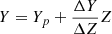 with the primordial helium abundance Yp = 0.2471 from Planck Collaboration VI (2020). The helium-to-metal enrichment ratio ΔY/ΔZ was set to 2.0. α enhancement was considered for α elements and Al. For every element X, we adapted a linear model to the evolution [X/Fe] with [α/Fe] as reported in V24. The values cX of these slopes (Table 1) were used to describe the variation of individual elements with [α/Fe]: [X/Fe] = cX × [α/Fe]. Stellar models were computed for [α/Fe] from −0.1 to 0.4 with a step of 0.1 dex.
Dependence of the different element abundances [X/Fe] on [α/Fe].
Models were computed with the FRANEC code. The input physics was the same as that adopted to compute the Pisa Stellar Evolution Data Base1 for low-mass stars (Dell’Omodarme et al. 2012), apart from the following differences. The outer boundary conditions were set by the Vernazza et al. (1981) solar semi-empirical T(τ), which well approximate the results obtained using the hydro-calibrated T(τ) (Salaris & Cassisi 2015; Salaris et al. 2018). The models were computed assuming the solar-scaled mixing-length parameter αMLT = 1.91. A moderate mass-loss was assumed according to the parametrisation by Reimers (1975), with an efficiency of η = 0.2. High-temperature (T > 10 000 K) radiative opacities were taken from the OPAL group (Rogers et al. 1996), whereas for lower temperatures the code adopts molecular opacities by Marigo et al. (2022)2. Both high- and low-temperature opacity tables account for the metal distributions adopted in the computations.
Raw stellar evolutionary tracks were reduced to a set of tracks with the same number of homologous points according to the evolutionary phase. Details about the reduction procedure are reported in the Appendix of Valle et al. (2013). Only models in RGB with 1.4 ≤ log g ≤ 3.3 and an age of below 14 Ga were retained in the final grid.
2.2. Effective temperature discrepancies
For each star in the sample, we compared the observed effective temperature Teff, obs with a theoretical value Teff, mod estimated by linearly interpolating over the grid of stellar models. The interpolation was carried out in mass, log g, [α/Fe], and [Fe/H]. The difference between the observed and estimated temperatures defines the effective temperature offset, ΔT = Teff, obs − Teff, mod. Stellar masses used in the process were derived from asteroseismic scaling relations and sourced from the APO-K2 catalogue. These mass estimates apply a correction to the face Δν values used in the scaling relations, with the coefficient fΔν derived from Sharma et al. (2016). It is therefore important to acknowledge that a possible uncontrolled systematic bias present in these estimates may affect the obtained results. Correction factor variations of up to 2% are reported in the literature along with possible systematic trends related to stellar mass, metallicity, and log g (Li et al. 2022, 2023). While a thorough investigation of these effects across different correction methods would be desirable, it falls outside the scope of this paper.
Our approach is the same as that adopted by Tayar et al. (2017) and Salaris et al. (2018), who performed the analysis using different stellar models over a smaller sample of RGB stars. Therefore, a direct comparison of the results could deepen our understanding of the discrepancies between stellar models and observations, and particularly with regard to how these discrepancies vary with different parameters such as [Fe/H] or [α/Fe].
2.3. Statistical models
Previous studies (e.g. Tayar et al. 2017; Salaris et al. 2018; Valle et al. 2019) have explored the relationship between effective temperature offset ΔT and metallicity [Fe/H] or α enhancement. However, they might not fully account for biases arising from differences in stellar populations across the [Fe/H]–[α/Fe] plane. For instance, variations in stellar mass distributions at different [α/Fe] values could distort the results. To address this, a multivariate approach is needed that considers the interplay between multiple variables simultaneously. This is particularly important because investigations into marginalised trends of ΔT can lead to misleading conclusions given the hidden influences from other neglected factors. In our analysis, we use a generalised additive model (GAM, Hastie & Tibshirani 1986; Wood 2017) to capture potential non-linear relationships between ΔT and various observational parameters.
GAMs extend generalised linear models by allowing the response variable Y to depend on smooth, unknown functions of the predictor variables x. These functions do not need a predefined form, and the optimal level of smoothness for each is automatically determined by the model. The general GAM form is:
 (1)
(1)
where g(.) is a link function, μi = 𝔼(Yi) are the expected values of Yi, and Yi ∼ EF(μi, ϕ), where EF(μi, ϕ) is an exponential family distribution with mean μi and scale parameter ϕ. Also, Ai is a row of the model matrix for any parametric model components, θ is the corresponding parameter vector, and fj(.) are smooth functions of the different subsets Sj of the covariates x. The smoothing functions fj(.) are then expanded over a basis of functions, which are completely known. If bj(x) is the j-th such basis function, then f(.) are assumed to have a representation
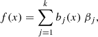 (2)
(2)
where βj are unknown parameters and k is the basis space dimension. We estimated the smooth functions in the model using penalised regression methods. The degree of smoothness was automatically determined from the data using the generalised cross-validation criterion as described in Wood (2017). We used the gam function from the mgcv package in R 4.3.2 (R Core Team 2023) to fit the model. This function employs penalised regression splines with basis functions optimised for the chosen number of basis functions (Wood 2017).
The fitted model was
![Mathematical equation: $$ \begin{aligned} \Delta T = f_1(\mathrm{[Fe/H]} , [\alpha /\mathrm{Fe}] , \log g) + f_2(M) + [\alpha /\mathrm{Fe}]*\mathrm{[Fe/H]}*M ,\end{aligned} $$](/articles/aa/full_html/2024/10/aa51730-24/aa51730-24-eq4.gif) (3)
(3)
where the asterisk in the model specification indicates that we fit not only the individual terms but also their interactions, capturing potential combined effects. This results in a model with three components: a parametric component for the interaction term ([α/Fe]*[Fe/H] * M), a smoothing function of the mass M, and a multivariate smoothing function of [Fe/H], [α/Fe], and log g. The adequacy of the chosen base dimensions for the smoothing functions was verified using the k′ test (Wood 2017).
To ensure the robustness of our conclusions, we additionally fit an alternative model using projection pursuit regression (Venables & Ripley 2002); simar. However, both models yielded similar predictions. Therefore, we only present the results based on the GAM model.
2.4. Age-fitting technique
The analysis was conducted adopting the SCEPtER pipeline3, a well-tested technique for fitting single and binary systems (e.g. Valle et al. 2014, 2015b, 2023). The pipeline estimates the stellar age adopting a grid maximum likelihood approach, relying on the observed quantities o ≡ {Teff, [Fe/H], Δν, νmax}. For every star, a fitting grid with [α/Fe] equal to the observed values is obtained by means of linear interpolation. Then, for every j-th point in the fitting grid, a likelihood estimate is obtained
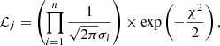 (4)
(4)
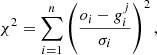 (5)
(5)
where oi are the n observational constraints, gij are the j-th grid point corresponding values, and σi are the observational uncertainties. The estimated stellar ages were obtained by averaging the age of all the models with a likelihood of greater than 0.95 × Lmax4. The confidence interval for these estimates was obtained by means of a Monte Carlo simulation. We repeated the estimation over a generated sample of size n = 1000 for every star. These synthetic stars were obtained by means of Gaussian perturbations around their observed values, adopting a diagonal covariance matrix Σ = diag(σ2). The median of the n ages was taken as the best estimate of the true values; the 16th and 84th percentiles of the n values were adopted as a 1σ confidence interval.
Nevertheless, concerns have been raised regarding the use of effective temperature as a constraint in fitting procedures due to both observational and theoretical uncertainties (see e.g. Martig et al. 2015; Warfield et al. 2021; Vincenzo et al. 2021). Biases in effective temperature values relative to the fitting grid can significantly impact estimated ages through their influence on mass, which directly affects age determination. To deal with this issue, we adopted Teff, mod, the theoretical interpolated effective temperatures, as observational constraints in the fit (Martig et al. 2015; Warfield et al. 2021, 2024).
3. Test of stellar models
3.1. Marginalised univariate investigations
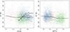 |
Fig. 1. Effective temperature difference between observations and models as a function of different observational parameters. Left: ΔT vs [Fe/H]. Colours identify stars as in the APO-K2 catalogue (green = high α, blue = low α, red = transition). The black solid line represent a loess smoothing of the data. Open circles show the trend reported in Salaris et al. (2018), while open triangles show the trend by Tayar et al. (2017), shifted downward by 100 K. Right: Same as in the left panel but as a function of [α/Fe]. |
Figure 1 presents the difference between observed and predicted effective temperatures ΔT as a function of metallicity [Fe/H] and [α/Fe]. Overall, the trend with [Fe/H] suggests a slight systematic bias in the models, with a median overprediction of temperature by about 35 K. This trend remains relatively flat across the metallicity range. The left panel also shows the trends reported by Tayar et al. (2017) and Salaris et al. (2018) for comparison. The values from Tayar et al. (2017) were rebinned as in Salaris et al. (2018) and shifted downward by 100 K for an easy visual comparison. Our results differ significantly from those of the previous studies. The stellar evolution code adopted here is very similar to that by Salaris et al. (2018), the main difference being the correction of the element trend with [α/Fe]. However, definitively attributing the differences in the ΔT agreement solely to this specific modification would be premature. As the following discussion shows, other factors like the underlying distributions of [α/Fe], mass, and log g in stars across different [Fe/H] intervals could also influence this trend. Moreover, it is relevant to note that the analyses of Tayar et al. (2017) and Salaris et al. (2018) were based upon APOGEE DR13 data, and several differences have arisen in the APOGEE fitting and calibration pipeline since those studies (Holtzman et al. 2018; Jönsson et al. 2020). The effective temperatures provided in the APOGEE DR17 data set used in this paper were calibrated based on the work by González Hernández & Bonifacio (2009). This calibration successfully removed a significant dependence of the spectroscopic Teff on the metallicity [Fe/H]. A comparison of these calibrated effective temperatures with those from other catalogues (Hegedűs et al. 2023) did not reveal any significant residual trends or biases, further supporting the robustness of the analysis presented here.
The right panel of Fig. 1 presents ΔT values against [α/Fe], highlighting the model’s differing accuracy at low and high α-values. Stars with high α enhancement exhibit a roughly 50 K disagreement with the model, while the discrepancy is only about 25 K for stars with low α enhancement. The difference in accuracy as a function of [α/Fe] aligns with the finding by Salaris et al. (2018), who reported improved agreement in ΔT when restricting to [α/Fe]< 0.07 stars. However, the same caveat as that mentioned for [Fe/H] trend regarding premature conclusions applies here as well. Interestingly, repeating the analysis with the uncalibrated APOGEE temperature TEFF_SPEC revealed a significantly larger discrepancy of 56 K between the two groups. This discrepancy also showed a steep dependence of ΔT on [α/Fe], suggesting that the residual difference between the low- and high-α populations might, at least partially, originate from an inhomogeneous calibration across the entire [α/Fe] range.
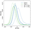 |
Fig. 2. Kernel density estimator of the ΔT distribution in low- and high-α populations (solid lines). Dashed lines show the distributions restricted to M < 1.0 M⊙, while dotted lines correspond to M > 1.0 M⊙ populations. |
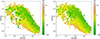 |
Fig. 3. Two-dimensional plot of ΔT as a function of [Fe/H] and [α/Fe]. The black dashed line marks the separation adopted in the APO-K2 catalogue to define low- and high-α populations. Left: Map of the observed differences. Right: Map of the differences as predicted by GAM model. |
Figure 2 displays the kernel density estimators of the differences in predicted effective temperature accuracy for high- and low-α populations. The figure also shows the kernel density estimator in the subpopulations obtained by separating stars according to their mass, adopting 1.0 M⊙ for the cut. For both populations, ΔT values are consistently higher by about 25 K in lower mass bins. This trend contradicts the findings of Tayar et al. (2017), who reported a positive linear correlation (Pearson coefficient r = 0.12) between mass and ΔT. Our analysis yields a negative correlation (r = −0.23), but the strong nonlinearity in the data suggests this value may not be meaningful. Furthermore, the analysed sample lacks homogeneity within the observational hyperspace, introducing potential biases due to uncontrolled confounding variables in marginalised analyses. For instance, the observed mass dependence of ΔT is particularly relevant considering the significant mass differences between high- and low-α populations. The low-α group has a median mass of 1.18 M⊙ (interquartile range [1.08, 1.30] M⊙), while the high-α stars have a median of 0.98 M⊙ (interquartile range [0.92, 1.06] M⊙). This disparity could significantly bias the results of marginalised analyses presented earlier.
3.2. Non-linear multivariate approach
To deal with this fundamental question and disentangle the contributions from the different stellar observables to the ΔT value, a robust and multivariate approach is mandatory. We adopt a GAM for this analysis, as detailed in Section 2.3. This model class offers superior flexibility compared to linear models, enabling both accurate predictions and the avoidance of overfitting (Wood 2017). The adequacy of the fitted GAM, specified in Eq. (3), is evaluated in Appendix A.
The first test of the model is its capability to reproduce the ΔT values across the [α/Fe] versus [Fe/H] plane. In the left panel of Fig. 3, a filled contour plot of the ΔT in this plane is shown (a positive ΔT value means that the observed temperature is greater than the theoretical one). The plot was produced by computing the mean value of the neighbourhood stars ΔT over a regular grid. A bidimensional rectangular kernel with bandwidths from Sheather & Jones (1991) is adopted for the mean computation. It is apparent that models become hotter moving from the low- to the high-α groups, with a reduced trend within the two groups. The plot shows that the ΔT values evolve mostly parallel to the separation line adopted in the APO-K2 catalogue to identify low- and high-α populations. The same plot is shown in the right panel of Fig. 3 but this time using ΔT values as predicted by GAM. While adjusting a few outliers in the real data, the model demonstrably aligns with observed trends, supporting the credibility of its predictions.
The availability of a reliable statistical model allows us to explore the individual contributions of the different stellar parameters to ΔT. The interpretation of the trend seen in Fig. 3 is indeed complex because the mass distribution significantly differs as a function of [Fe/H] and [α/Fe]. A much clearer view would result from filtering out this confounding factor. Using the GAM to predict ΔT while assigning the same mass and log g value to all the stars would reveal the actual trend of ΔT with [Fe/H] and [α/Fe]. Moreover, comparing the results produced by fixing the stellar mass to different values would help us to clarify the trends in mass given [Fe/H] and [α/Fe]. To this aim, Fig. 4 shows the maps obtained by fixing stellar masses to 0.9 and 1.2 M⊙ and log g = 2.7.
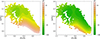 |
Fig. 4. Two-dimensional plot of ΔT from GAM predictions as a function of [Fe/H] and [α/Fe] when fixing the masses to different values. Left: Stellar masses set to 0.9 M⊙. Right: Stellar masses set to 1.2 M⊙. |
The analysis of this figure reveals three key findings regarding the discrepancies between models and observations.
-
The two maps exhibit notable variations in ΔT as a function of stellar mass for the same zone in the [α/Fe] – [Fe/H] plane. This suggests that the model–observation agreement is mass-dependent, implying that changes in effective temperature between models at different masses do not correctly reflect observed changes.
-
The ΔT offset evolves strongly when moving along the [α/Fe] axis. At [Fe/H] = −0.5, there is a difference of about 100 K in the effective temperature offset between the extreme [α/Fe] zones. The ΔT dependence on [Fe/H] is weaker, with a typical maximum variation of about one-half of that due to [α/Fe].
-
The ΔT offset evolves nearly parallel to the line adopted in the separation of high- and low-α populations, in agreement with the evidence discussed above for the global map.
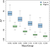 |
Fig. 5. Boxplot of ΔT as a function of the stellar mass and α enhancement group (L = low-α, H = high-α). |
Figure 5 further explores the dependence of ΔT on stellar mass. The boxplots show the distribution of effective temperature errors predicted by the GAM model when all data set masses are fixed. Stellar masses in the range from 0.9 M⊙ to 1.2 M⊙ are considered. This reveals a clear mass dependence in model accuracy, with the median ΔT varying by approximately 60 K between the maximum and minimum considered masses. The difference in effective temperature between low- and high-α populations slightly decreases with increasing mass from about 70 K to about 55 K. These values are significantly higher than the 25 K inferred from the analysis of the right panel in Fig. 1, highlighting the significance of mass as a confounding factor in univariate analyses.
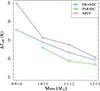 |
Fig. 6. Effective temperature differences between stellar models for a shift of 0.1 M⊙ in the range from 0.9 M⊙ to 1.3 M⊙. Symbols identify stellar models from different codes. The comparison is performed at [Fe/H] = 0.0, [α/Fe] = 0.0. |
The robustness of the ΔT dependence on stellar mass should be further investigated using different stellar evolutionary codes. The Teff computed by these codes is primarily influenced by the adopted boundary conditions and mixing-length parameter. Different choices lead to different offsets as a function of metallicity. This is demonstrated in the analysis presented by Salaris et al. (2018), who showed the effect of adopting different boundary conditions in the model computations. Consequently, effective temperatures from different codes are likely to have distinct zero points and potentially different gradients in the [α/Fe]–[Fe/H] plane. However, when all other inputs are held constant, the predicted difference in Teff for a given difference in stellar mass should be highly similar across various codes. This is because this differential effect is not influenced by variations in the adopted [α/Fe] and [Fe/H].
Figure 6 presents the difference in effective temperature at fixed log g = 2.75 for a 0.1 M⊙ increase in stellar mass and for baseline masses of 0.9, 1.0, 1.1, and 1.2 M⊙. We compare our FRANEC models with MIST models computed using MESA (Choi et al. 2016) and PARSEC models (Nguyen et al. 2022)5. The comparison is made at a common value of [α/Fe] = 0.0 and [Fe/H] = 0.0. Unfortunately, PARSEC and MIST databases lack models at different [α/Fe], limiting a more comprehensive comparison.
Despite differences in mixing-length parameters, solar reference mixtures, and boundary conditions, the temperature offset and its trend with stellar mass show remarkable similarity across the codes. Significant differences arise when comparing these data to those from observations. The temperature differences from observed data at [α/Fe] = 0.0 and [Fe/H] = 0.0, as resulting from the GAM model, are 6.0 ± 5.5 K (0.9–1.0 M⊙ shift) and 12.1 ± 5.2 K (1.2–1.3 M⊙ shift), compared to model predictions of about 30 K and 20 K, respectively. This suggests a significant discrepancy between the trend of APOGEE DR17 Teff with stellar mass and that from models. To investigate possible trends induced by the effective temperature calibration in the APOGEE data set, we repeated the analysis using the spectroscopic uncalibrated Teff, which revealed an interesting trend. Using spectroscopic data, the difference between 0.9 and 1.0 M⊙ (30 K) is in line with the expectation from stellar models. However, significant differences occur in the following bins, because the difference between uncalibrated effective temperatures decreases to only 7 K in the 1.2 to 1.3 M⊙ mass bin.
4. Grid-based age estimates
In the presence of the discrepancies between observed and predicted effective temperature, the direct adoption of grid-based estimates of stellar ages is quite problematic. As discussed, for example, by Martig et al. (2015) and Warfield et al. (2021), using the observed Teff to constrain stellar parameters would bias the estimated mass, thus biasing the age. Nevertheless, neglecting the Teff constraint is not advisable because, in its absence, grid-based estimates for RGB stars are affected by large uncertainties (Pinsonneault et al. 2018). A possible remedy (Martig et al. 2015; Warfield et al. 2021, 2024) is to substitute the effective temperature constraint with that on the stellar mass, as estimated by asteroseismic scaling relations. The accuracy of the asteroseismic scaling relations has been extensively investigated and there is evidence of a metallicity, effective temperature, and evolutionary phase-dependent offset in the large frequency separation relation (e.g. White et al. 2011; Sharma et al. 2016; Stello & Sharma 2022; Li et al. 2022). Tests carried out on the scaling relations suggest they are accurate to a level of a few percent (e.g. Miglio et al. 2016; Rodrigues et al. 2017; Brogaard et al. 2018; Buldgen et al. 2019). The approach of fixing the stellar mass to its asteroseismic value is equivalent to adopting the model-predicted effective temperature for the mass given by the scaling relation, log g being fixed to the observational constraint. In this section, we adopt this method to estimate the age of the RGB star in our sample.
Grid-based estimates of age, mass, and radius for the selected RGB stars.
Caution is urged when interpreting age estimates derived from this approach. This method implicitly assumes that unknown factors solely affecting temperature and not evolutionary timescale explain the observed discrepancy in effective temperature. The two primary candidates for such factors are boundary conditions and the mixing-length parameter (Tayar et al. 2017; Salaris et al. 2018). Consequently, the reliability of these age estimates depends on the validity of the underlying assumption.
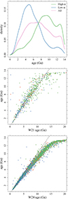 |
Fig. 7. Grid-based estimates of stellar ages. Top: Kernel-density estimators of the age distribution in the full sample (purple line) and in the high- and low-α populations (green and blue lines, respectively). Middle: Comparison of the age estimates from the present paper to those from W21. Bottom: Comparison of the age estimates from the present paper to those from W24. |
As expected, grid-based estimates of masses and radii are consistent with those from scaling relations. The distribution of relative errors in mass estimates has a median of 0.4% and a dispersion characterised by the 16th and 84th percentiles of [−0.7%, 1.9%]. The median relative error in radius estimates is 0.4% [−0.2%, 1.8%]. Both distributions show a positive skewness characteristic of RGB grid-based estimates (Gai et al. 2011; Valle et al. 2015a).
Figure 7 presents the age estimates of the stars. Consistent with previous findings, the age distributions between the low- and high-α groups differ significantly (top panel). The low-α group peaks at around 5 Ga, while the high-α population peaks at around 9 Ga. The analysis confirms the presence of a significant fraction of young and intermediate-age stars (approximately 6% younger than 4 Ga and 15% younger than 6 Ga) in the high-α population, consistent with previous findings (e.g. Chiappini et al. 2015; Warfield et al. 2021; Zinn et al. 2022; Warfield et al. 2024). The origin of these stars is still debated. Some authors propose that they are indeed old stars that appear young after a merger (e.g. Martig et al. 2015; Jofré et al. 2016; Izzard et al. 2018; Sun et al. 2020; Grisoni et al. 2024), others suggest that they are genuinely young and formed in gas relatively unenriched by SNe Ia (e.g. Chiappini et al. 2015; Johnson et al. 2021) or from bursts of star formation that enhance the rate of core-collapse supernovae enrichment (Johnson & Weinberg 2020). Overall, the age distributions in Fig. 7 closely resemble those found by Warfield et al. (2021) and Zinn et al. (2022).
The middle and bottom panels of Fig. 7 show comparisons of our age estimates with those from Warfield et al. (2021) (W21) and Warfield et al. (2024) (W24), respectively. The comparisons are performed over the samples of common stars, which contain 655 and 4246, respectively. To enhance readability, error bars are omitted from the figure (the typical 1σ error in age is similar for all datasets, being approximately 2 Ga). The age estimates exhibit good agreement at low age, with only a few stars showing a significantly different prediction. A noticeable disagreement occurs at high ages, possibly due to the difference in the estimation methods. While we impose a cut off of 14 Ga to the models in the grid, no such limit exists in the W21 and W24 grids. Consequently, in their data set, there are stars with estimated ages of more than 20 Ga. Therefore, this comparison cannot shed light on the importance of the differences in chemical evolution profiles employed in these studies. A star-by-star comparison, restricted to stars younger than 14 Ga in both W21 and W24, reveals that our estimates are higher by approximately 0.3 Ga and lower by 0.6 Ga with respect to W21 and W24, respectively. These discrepancies mainly arise for stars older than about 10 Ga, where the different age boundary imposed in the fit becomes relevant.
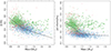 |
Fig. 8. Evolution of surface abundance of different elements with stellar mass. Left: [C/N] ratio evolution. The dashed line shows the predictions from stellar models. The larger symbols identify young α-rich stars according to the Grisoni et al. (2024) classification. Right: Same as in the left panel but for the [(C+N+O)/Fe] ratio trend. |
Despite the global agreement in age estimates, especially for low ages, it is important to note that this is due to a coincidental cancellation effect. Important differences exist in the element scaling with [α/Fe] between our investigation and those in the literature such as Martig et al. (2015), Warfield et al. (2021), Miglio et al. (2021), and Warfield et al. (2024). The chemical composition adopted in the present paper for high-α stars becomes progressively O-rich with increasing [α/Fe]. Simultaneously, the modified composition also impacts the [Fe/H]-to-Z relation. By chance, the two effects have a nearly opposite influence on the stellar evolution timescale, causing age estimates to appear similar even if the underlying assumptions are very different.
Figure 8 shows the evolution of [C/N] and [(C+N+O)/Fe] ratios with stellar mass. For each star, the surface abundances of C, N, and O were estimated from a grid-based fit. The agreement between theoretical models and observations is generally good. The model-predicted [C/N] ratios are systematically lower than the observed values by about 0.04 dex. This difference is less than half of what is expected from variations in computational algorithms used by different stellar evolutionary codes (Silva Aguirre et al. 2020). The discrepancy is even smaller for the predicted and observed [(C+N+O)/Fe] ratios, with a median difference of 0.01 dex. The figure helps us to investigate on the young population among the high-α stars. These stars were identified as in Chiappini et al. (2015) and Grisoni et al. (2024), relying on estimated ages and the [Mg/Fe] ratio. Represented by larger symbols in the figure, the high-α young stars clearly deviate from the predicted trends. A star-by star comparison reveals that the [C/N] median difference between observations and models is 0.24 dex in the high-α young population, while it is 0.08 dex in the high-α old group. This discrepancy is often attributed to mergers or mass-transfer events between two lower-mass giants, which have preserved their original [C/N] values (Chiappini et al. 2015; Jofré et al. 2016; Grisoni et al. 2024). Therefore, age estimates for this group are questionable.
5. Conclusions
Leveraging the recently released APO-K2 catalogue (Schonhut-Stasik et al. 2024), we performed an investigation of the agreement between stellar model predictions and observations for RGB stars. To this purpose, we adopted the element scaling with [α/Fe] as resulting from the analysis of V24. The most notable correction is a trend between oxygen and [α/Fe] that is steeper than assumed in a uniform α enhancement scenario.
The difference in the mixture scaling with [α/Fe] impacts stellar models in several ways. First, it alters the evolutionary timescale and the [Fe/H]-to-Z relationship, potentially affecting age estimates from stellar models. Second, it modifies the opacity of stellar matter, consequently influencing the predicted effective temperatures. These modifications have the potential to significantly change the current paradigm regarding the agreement between stellar models and observations (e.g. Tayar et al. 2017; Salaris et al. 2018; Valle et al. 2019), and age estimates for high- and low-α stellar populations (e.g. Martig et al. 2015; Warfield et al. 2021, 2024; Miglio et al. 2021).
Univariate investigations showed significant differences in the ΔT offset between data and models with respect to previous investigations by Tayar et al. (2017) and Salaris et al. (2018). Our analysis does not evidence the ΔT trend with [Fe/H] discussed in the literature. Moreover, the ΔT trend with stellar mass is reversed with respect to the Tayar et al. (2017) analysis. A slight difference in ΔT of 25 K was detected between high- and low-α populations.
However, these analyses – which are commonly presented in the literature – are potentially misleading. The differences in the stellar mass and log g distributions at different [Fe/H] and [α/Fe] values may act as hidden confounding variables. To address this issue, we employed a non-linear multivariate statistical model, specifically a generalised additive model (GAM; Hastie & Tibshirani 1986; Wood 2017) with two smooth terms and a parametric component. This GAM captured the complex relationships between stellar parameters and identified their contributions to ΔT model-to-data discrepancies.
Our analysis reveals the following key findings.
-
The ΔT changes with stellar mass, deviating from model predictions. For a mass increase from 0.9 M⊙ to 1.2 M⊙ (while holding other parameters fixed), the median ΔT decreases by roughly 55 K. This suggests that changes in effective temperature between models at different masses do not correctly reflect observed changes.
-
The ΔT offset has a strong evolution moving along the [α/Fe] axis. At [Fe/H] = −0.5, there is a difference of about 100 K in the effective temperature offset between the extreme [α/Fe] zones. The ΔT dependence on [Fe/H] is about one half of that due to [α/Fe].
-
The direction of the steepest ΔT change is almost orthogonal to the line adopted in the separation of high- and low-α populations.
Therefore, adopting the scaling of the stellar composition with [α/Fe] that mimics the observed trends does not remove the discrepancies between models and predictions; however, it does rule out the possibility that a mismatch in the chemical composition evolution with [α/Fe] is the main responsible factor and helps us to assess the contribution of different stellar parameters to this disagreement. It is well established that the predicted effective temperatures of RGB stars in stellar models are highly sensitive to the chosen boundary conditions and the mixing-length parameter. These factors have been implicated as potential contributors to the observed discrepancies between theoretical predictions and observed Teff values (Tayar et al. 2017; Salaris et al. 2018). However, a definitive solution to this problem remains elusive. Further theoretical development and alternative approaches might help to reconcile theory and observations (e.g. Mosumgaard et al. 2020; Spada et al. 2021; Joyce & Tayar 2023).
Due to discrepancies between observed and modelled effective temperatures, using them directly to constrain stellar ages is unreliable. Therefore, we adopted an approach similar to the one by Martig et al. (2015), Warfield et al. (2021), and Warfield et al. (2024). We adopted model-derived effective temperatures for the grid-based age estimation, utilising the stellar mass from the asteroseismic scaling relation to interpolate the model effective temperature. The resulting age estimates are consistent with those reported in the literature (e.g. Martig et al. 2015; Warfield et al. 2021, 2024; Miglio et al. 2021), confirming the presence of a 6% fraction of stars younger than 4 Ga in the high-α population. A star-by-star comparison with W21 reveals a median difference of 0.4 Ga, with our estimates generally higher. The same comparison with W24 shows a median difference of -0.6 Ga for stars younger than 14 Ga in both data sets. Analyses of the [C/N] ratio support a possible origin of the young high-α population in mergers or mass-transfer events (Chiappini et al. 2015; Grisoni et al. 2024).
While our estimated ages globally agree with previous results, this agreement comes from a serendipitous cancellation effect. Our investigations rely on stellar models computed under different chemical abundances and input physics. Notably, the chemical composition adopted in our analysis becomes progressively O-rich increasing [α/Fe] with respect to a standard α enhancement scenario. This also modifies the [Fe/H]-to-Z relationship. By chance, the two effects have a nearly opposite impact on the stellar evolution timescale, resulting in very similar age estimates even if the underlying assumptions are very different. The resilience of age estimates to changes in the scaling between chemical abundance and [α/Fe] bolsters our confidence in the findings of the existing literature.
Data availability
The full Table 2 is available at the CDS via anonymous ftp to cdsarc.cds.unistra.fr (130.79.128.5) or via https://cdsarc.cds.unistra.fr/viz-bin/cat/J/A+A/690/A323
Publicly available on CRAN: http://CRAN.R-project.org/package=SCEPtER
The likelihood threshold is set for computational efficiency. Negligible differences arise using a weighted mean where each model’s weight reflects its likelihood.
PARSEC lacks models for 0.9 M⊙ in the most recent version of the database.
Acknowledgments
G.V., P.G.P.M. and S.D. acknowledge INFN (Iniziativa specifica TAsP) and support from PRIN MIUR2022 Progetto "CHRONOS" (PI: S. Cassisi) finanziato dall’Unione Europea - Next Generation EU.
References
- Abdurro’uf, Accetta, K., Aerts, C., et al. 2022, ApJS, 259, 35 [NASA ADS] [CrossRef] [Google Scholar]
- Amarsi, A. M., Nissen, P. E., & Skúladóttir, Á. 2019, A&A, 630, A104 [NASA ADS] [CrossRef] [EDP Sciences] [Google Scholar]
- Asplund, M., Grevesse, N., Sauval, A. J., & Scott, P. 2009, ARA&A, 47, 481 [NASA ADS] [CrossRef] [Google Scholar]
- Basu, S., Chaplin, W. J., & Elsworth, Y. 2010, ApJ, 710, 1596 [NASA ADS] [CrossRef] [Google Scholar]
- Basu, S., Verner, G. A., Chaplin, W. J., & Elsworth, Y. 2012, ApJ, 746, 76 [NASA ADS] [CrossRef] [Google Scholar]
- Bensby, T., Feltzing, S., Lundström, I., & Ilyin, I. 2005, A&A, 433, 185 [NASA ADS] [CrossRef] [EDP Sciences] [Google Scholar]
- Bertran de Lis, S., Delgado Mena, E., Adibekyan, V. Z., Santos, N. C., & Sousa, S. G. 2015, A&A, 576, A89 [NASA ADS] [CrossRef] [EDP Sciences] [Google Scholar]
- Böhm-Vitense, E. 1958, Z. Astrophys., 46, 108 [Google Scholar]
- Brogaard, K., Hansen, C. J., Miglio, A., et al. 2018, MNRAS, 476, 3729 [Google Scholar]
- Buldgen, G., Rendle, B., Sonoi, T., et al. 2019, MNRAS, 482, 2305 [Google Scholar]
- Chiappini, C., Anders, F., Rodrigues, T. S., et al. 2015, A&A, 576, L12 [NASA ADS] [CrossRef] [EDP Sciences] [Google Scholar]
- Choi, J., Dotter, A., Conroy, C., et al. 2016, ApJ, 823, 102 [Google Scholar]
- Dell’Omodarme, M., Valle, G., Degl’Innocenti, S., & Prada Moroni, P. G. 2012, A&A, 540, A26 [CrossRef] [EDP Sciences] [Google Scholar]
- Gai, N., Basu, S., Chaplin, W. J., & Elsworth, Y. 2011, ApJ, 730, 63 [Google Scholar]
- Gaia Collaboration (Brown, A. G. A., et al.) 2021, A&A, 649, A1 [NASA ADS] [CrossRef] [EDP Sciences] [Google Scholar]
- González Hernández, J. I., & Bonifacio, P. 2009, A&A, 497, 497 [Google Scholar]
- Grisoni, V., Chiappini, C., Miglio, A., et al. 2024, A&A, 683, A111 [NASA ADS] [CrossRef] [EDP Sciences] [Google Scholar]
- Härdle, W. K., & Simar, L. 2012, Applied Multivariate Statistical Analysis (Springer) [CrossRef] [Google Scholar]
- Hastie, T., & Tibshirani, R. 1986, Stat. Sci., 1, 297 [Google Scholar]
- Hegedűs, V., Mészáros, S., Jofré, P., et al. 2023, A&A, 670, A107 [NASA ADS] [CrossRef] [EDP Sciences] [Google Scholar]
- Holtzman, J. A., Hasselquist, S., Shetrone, M., et al. 2018, AJ, 156, 125 [Google Scholar]
- Izzard, R. G., Preece, H., Jofre, P., et al. 2018, MNRAS, 473, 2984 [NASA ADS] [CrossRef] [Google Scholar]
- Jofré, P., Jorissen, A., Van Eck, S., et al. 2016, A&A, 595, A60 [Google Scholar]
- Johnson, J. W., & Weinberg, D. H. 2020, MNRAS, 498, 1364 [CrossRef] [Google Scholar]
- Johnson, J. W., Weinberg, D. H., Vincenzo, F., et al. 2021, MNRAS, 508, 4484 [NASA ADS] [CrossRef] [Google Scholar]
- Jönsson, H., Holtzman, J. A., Allende Prieto, C., et al. 2020, AJ, 160, 120 [Google Scholar]
- Joyce, M., & Tayar, J. 2023, Galaxies, 11, 75 [NASA ADS] [CrossRef] [Google Scholar]
- Li, T., Li, Y., Bi, S., et al. 2022, ApJ, 927, 167 [NASA ADS] [CrossRef] [Google Scholar]
- Li, Y., Bedding, T. R., Stello, D., et al. 2023, MNRAS, 523, 916 [NASA ADS] [CrossRef] [Google Scholar]
- Marigo, P., Aringer, B., Girardi, L., & Bressan, A. 2022, ApJ, 940, 129 [NASA ADS] [CrossRef] [Google Scholar]
- Martig, M., Rix, H.-W., Silva Aguirre, V., et al. 2015, MNRAS, 451, 2230 [NASA ADS] [CrossRef] [Google Scholar]
- Miglio, A., Chiappini, C., Morel, T., et al. 2013, MNRAS, 429, 423 [Google Scholar]
- Miglio, A., Chaplin, W. J., Brogaard, K., et al. 2016, MNRAS, 461, 760 [NASA ADS] [CrossRef] [Google Scholar]
- Miglio, A., Chiappini, C., Mackereth, J. T., et al. 2021, A&A, 645, A85 [NASA ADS] [CrossRef] [EDP Sciences] [Google Scholar]
- Miglio, A., Chiappini, C., Mosser, B., et al. 2017, Astron. Nachr., 338, 644 [Google Scholar]
- Mosumgaard, J. R., Jørgensen, A. C. S., Weiss, A., Silva Aguirre, V., & Christensen-Dalsgaard, J. 2020, MNRAS, 491, 1160 [Google Scholar]
- Nguyen, C. T., Costa, G., Girardi, L., et al. 2022, A&A, 665, A126 [NASA ADS] [CrossRef] [EDP Sciences] [Google Scholar]
- Nissen, P. E., Chen, Y. Q., Carigi, L., Schuster, W. J., & Zhao, G. 2014, A&A, 568, A25 [NASA ADS] [CrossRef] [EDP Sciences] [Google Scholar]
- Pinsonneault, M. H., Elsworth, Y., Epstein, C., et al. 2014, ApJS, 215, 19 [Google Scholar]
- Pinsonneault, M. H., Elsworth, Y. P., Tayar, J., et al. 2018, ApJS, 239, 32 [Google Scholar]
- Planck Collaboration VI. 2020, A&A, 641, A6 [NASA ADS] [CrossRef] [EDP Sciences] [Google Scholar]
- R Core Team 2023, R: A Language and Environment for Statistical Computing (Vienna, Austria: R Foundation for Statistical Computing) [Google Scholar]
- Reimers, D. 1975, Mem. Soc. Roy. Sci. Liege, 8, 369 [Google Scholar]
- Rodrigues, T. S., Bossini, D., Miglio, A., et al. 2017, MNRAS, 467, 1433 [NASA ADS] [Google Scholar]
- Rogers, F. J., Swenson, F. J., & Iglesias, C. A. 1996, ApJ, 456, 902 [Google Scholar]
- Salaris, M., & Cassisi, S. 1996, A&A, 305, 858 [NASA ADS] [Google Scholar]
- Salaris, M., & Cassisi, S. 2015, A&A, 577, A60 [CrossRef] [EDP Sciences] [Google Scholar]
- Salaris, M., Cassisi, S., Schiavon, R. P., & Pietrinferni, A. 2018, A&A, 612, A68 [NASA ADS] [CrossRef] [EDP Sciences] [Google Scholar]
- Schonhut-Stasik, J., Zinn, J. C., Stassun, K. G., et al. 2024, AJ, 167, 50 [NASA ADS] [CrossRef] [Google Scholar]
- Sharma, S., Stello, D., Bland-Hawthorn, J., Huber, D., & Bedding, T. R. 2016, ApJ, 822, 15 [Google Scholar]
- Sheather, S. J., & Jones, M. C. 1991, J. Roy. Stat. Soc., Ser. B Methodol., 53, 683 [Google Scholar]
- Silva Aguirre, V., Christensen-Dalsgaard, J., Cassisi, S., et al. 2020, A&A, 635, A164 [NASA ADS] [CrossRef] [EDP Sciences] [Google Scholar]
- Spada, F., Demarque, P., & Kupka, F. 2021, MNRAS, 504, 3128 [NASA ADS] [CrossRef] [Google Scholar]
- Stello, D., & Sharma, S. 2022, Res. Notes Am. Astron. Soc., 6, 168 [Google Scholar]
- Stello, D., Huber, D., Sharma, S., et al. 2015, ApJ, 809, L3 [NASA ADS] [CrossRef] [Google Scholar]
- Straniero, O., & Chieffi, A. 1991, ApJS, 76, 525 [NASA ADS] [CrossRef] [Google Scholar]
- Sun, W. X., Huang, Y., Wang, H. F., et al. 2020, ApJ, 903, 12 [NASA ADS] [CrossRef] [Google Scholar]
- Tayar, J., Somers, G., Pinsonneault, M. H., et al. 2017, ApJ, 840, 17 [NASA ADS] [CrossRef] [Google Scholar]
- Valle, G., Dell’Omodarme, M., Prada Moroni, P. G., & Degl’Innocenti, S. 2013, A&A, 549, A50 [CrossRef] [EDP Sciences] [Google Scholar]
- Valle, G., Dell’Omodarme, M., Prada Moroni, P. G., & Degl’Innocenti, S. 2014, A&A, 561, A125 [NASA ADS] [CrossRef] [EDP Sciences] [Google Scholar]
- Valle, G., Dell’Omodarme, M., Prada Moroni, P. G., & Degl’Innocenti, S. 2015a, A&A, 577, A72 [NASA ADS] [CrossRef] [EDP Sciences] [Google Scholar]
- Valle, G., Dell’Omodarme, M., Prada Moroni, P. G., & Degl’Innocenti, S. 2015b, A&A, 575, A12 [NASA ADS] [CrossRef] [EDP Sciences] [Google Scholar]
- Valle, G., Dell’Omodarme, M., Prada Moroni, P. G., & Degl’Innocenti, S. 2019, A&A, 623, A59 [NASA ADS] [CrossRef] [EDP Sciences] [Google Scholar]
- Valle, G., Dell’Omodarme, M., Prada Moroni, P. G., & Degl’Innocenti, S. 2020, A&A, 635, A77 [NASA ADS] [CrossRef] [EDP Sciences] [Google Scholar]
- Valle, G., Dell’Omodarme, M., Prada Moroni, P. G., & Degl’Innocenti, S. 2023, A&A, 678, A203 [NASA ADS] [CrossRef] [EDP Sciences] [Google Scholar]
- Valle, G., Dell’Omodarme, M., Prada Moroni, P. G., & Degl’Innocenti, S. 2024, A&A, 698, A159 [NASA ADS] [CrossRef] [EDP Sciences] [Google Scholar]
- Vandenberg, D. A., Bolte, M., & Stetson, P. B. 1996, ARA&A, 34, 461 [NASA ADS] [CrossRef] [Google Scholar]
- Venables, W., & Ripley, B. 2002, Modern applied statistics with S, Statistics and computing (Springer) [CrossRef] [Google Scholar]
- Vernazza, J. E., Avrett, E. H., & Loeser, R. 1981, ApJS, 45, 635 [Google Scholar]
- Vincenzo, F., Weinberg, D. H., Montalbán, J., et al. 2021, ArXiv e-prints [arXiv:2106.03912] [Google Scholar]
- Warfield, J. T., Zinn, J. C., Pinsonneault, M. H., et al. 2021, AJ, 161, 100 [NASA ADS] [CrossRef] [Google Scholar]
- Warfield, J. T., Zinn, J. C., Schonhut-Stasik, J., et al. 2024, AJ, 167, 208 [NASA ADS] [CrossRef] [Google Scholar]
- White, T. R., Bedding, T. R., Stello, D., et al. 2011, ApJ, 743, 161 [Google Scholar]
- Wood, S. N. 2017, Generalized Additive Models: An Introduction with R, 2nd edn. (CRC Press) [CrossRef] [Google Scholar]
- Yu, J., Khanna, S., Themessl, N., et al. 2023, ApJS, 264, 41 [NASA ADS] [CrossRef] [Google Scholar]
- Zinn, J. C., Stello, D., Elsworth, Y., et al. 2022, ApJ, 926, 191 [NASA ADS] [CrossRef] [Google Scholar]
Appendix A: Analysis of GAM residual
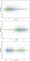 |
Fig. A.1. GAM residuals as a function of the stellar mass (in solar units), the metallicity [Fe/H], and [α/Fe]. The black lines are the smoother of the residuals. |
This section report the analysis of the adequacy of the GAM models in Eq. (3), adopted in the paper. The first check which should be performed for a GAM model is the adequacy of the basis dimension for the smooth terms. This test is based on computing an estimate of the residual variance based on differencing residuals that are near neighbours according to the covariates of the smooth (Wood 2017). This estimate, divided by the residual variance, is the k-index. The p-value is computed by simulation (Wood 2017). The results of the test are collected in Tab. A.1. The hypothesis of the adequacy of the base dimension cannot be rejected.
Adequacy test for the basis dimension for the two smooth terms.
The second test is the analysis of deviance residuals, to verify that the model correctly captured all the trends present in the data. Figure A.1 shows the model residuals as a function of the stellar mass, the metallicity [Fe/H], and [α/Fe], the smoother of the residuals, shown in the panels, demonstrate that no unaccounted trends are present in the model residuals.
The analysis of the model residuals shows the presence of 38 stars with residuals above 100 K that is, about 3σ above the mean. This high prevalence of outliers at high effective temperature suggests that these stars may possibly be RC stars, misclassified in the RGB group. In fact, the classification in the APO-K2 catalogue does not rely on robust asteroseismic detection of the period spacing but only on discriminating functions based on [C/N], log g, and Teff. However, the removal of these stars from the sample adopted for the GAM fit only marginally improve its performance and predictive capabilities. Therefore in the analysis we adopt the models computed without rejecting these potential outliers.
All Tables
All Figures
|
Fig. 1. Effective temperature difference between observations and models as a function of different observational parameters. Left: ΔT vs [Fe/H]. Colours identify stars as in the APO-K2 catalogue (green = high α, blue = low α, red = transition). The black solid line represent a loess smoothing of the data. Open circles show the trend reported in Salaris et al. (2018), while open triangles show the trend by Tayar et al. (2017), shifted downward by 100 K. Right: Same as in the left panel but as a function of [α/Fe]. |
| In the text | |
|
Fig. 2. Kernel density estimator of the ΔT distribution in low- and high-α populations (solid lines). Dashed lines show the distributions restricted to M < 1.0 M⊙, while dotted lines correspond to M > 1.0 M⊙ populations. |
| In the text | |
|
Fig. 3. Two-dimensional plot of ΔT as a function of [Fe/H] and [α/Fe]. The black dashed line marks the separation adopted in the APO-K2 catalogue to define low- and high-α populations. Left: Map of the observed differences. Right: Map of the differences as predicted by GAM model. |
| In the text | |
|
Fig. 4. Two-dimensional plot of ΔT from GAM predictions as a function of [Fe/H] and [α/Fe] when fixing the masses to different values. Left: Stellar masses set to 0.9 M⊙. Right: Stellar masses set to 1.2 M⊙. |
| In the text | |
|
Fig. 5. Boxplot of ΔT as a function of the stellar mass and α enhancement group (L = low-α, H = high-α). |
| In the text | |
|
Fig. 6. Effective temperature differences between stellar models for a shift of 0.1 M⊙ in the range from 0.9 M⊙ to 1.3 M⊙. Symbols identify stellar models from different codes. The comparison is performed at [Fe/H] = 0.0, [α/Fe] = 0.0. |
| In the text | |
|
Fig. 7. Grid-based estimates of stellar ages. Top: Kernel-density estimators of the age distribution in the full sample (purple line) and in the high- and low-α populations (green and blue lines, respectively). Middle: Comparison of the age estimates from the present paper to those from W21. Bottom: Comparison of the age estimates from the present paper to those from W24. |
| In the text | |
|
Fig. 8. Evolution of surface abundance of different elements with stellar mass. Left: [C/N] ratio evolution. The dashed line shows the predictions from stellar models. The larger symbols identify young α-rich stars according to the Grisoni et al. (2024) classification. Right: Same as in the left panel but for the [(C+N+O)/Fe] ratio trend. |
| In the text | |
|
Fig. A.1. GAM residuals as a function of the stellar mass (in solar units), the metallicity [Fe/H], and [α/Fe]. The black lines are the smoother of the residuals. |
| In the text | |
Current usage metrics show cumulative count of Article Views (full-text article views including HTML views, PDF and ePub downloads, according to the available data) and Abstracts Views on Vision4Press platform.
Data correspond to usage on the plateform after 2015. The current usage metrics is available 48-96 hours after online publication and is updated daily on week days.
Initial download of the metrics may take a while.