| Issue |
A&A
Volume 698, May 2025
|
|
|---|---|---|
| Article Number | A111 | |
| Number of page(s) | 6 | |
| Section | Stellar structure and evolution | |
| DOI | https://doi.org/10.1051/0004-6361/202554089 | |
| Published online | 03 June 2025 | |
The role of stellar model input in correcting the asteroseismic scaling relations
Red giant branch models
1
Dipartimento di Fisica “Enrico Fermi”, Università di Pisa, Largo Pontecorvo 3, I-56127 Pisa, Italy
2
INFN, Sezione di Pisa, Largo Pontecorvo 3, I-56127 Pisa, Italy
⋆ Corresponding author: valle@df.unipi.it
Received:
10
February
2025
Accepted:
25
April
2025
Aims. This study investigates the variability of the theoretical correction factor, fΔν, used in red giant branch (RGB) scaling relations, arising from different assumptions in stellar model computations.
Methods. Adopting a commonly used framework, we focused on a 1.0 M⊙ star and systematically varied seven input parameters: the reference solar mixture, the initial helium abundance, the inclusion of microscopic diffusion and mass loss, the method for calculating atmospheric opacity, the mixing-length parameter, and the boundary conditions. Each parameter was tested using two distinct but physically plausible values to mimic possible choices of different evolutionary codes. For each resulting stellar model, we computed the oscillation frequencies along the RGB and derived the large frequency spacing, Δν0. The correction factor fΔν was then calculated by comparing the derived Δν0 with that predicted by the uncorrected scaling relations.
Results. We found substantial variability in fΔν across the different models. The variation ranged from approximately 1.3% in the lower RGB to about 3% at log g = 1.4. This level of variability is significant, as it corresponds to roughly half the values typically quoted in the literature and leads to a systematic change in derived masses from 5% to more than 10%. The most significant contribution to this variability came from the choice of atmospheric opacity calculation (approximately 1.2%), with a smaller contribution from the inclusion of microscopic diffusion (approximately 0.4%).
Conclusions. These results indicate that the choice of the reference stellar model has a non-negligible impact on the calculation of correction factors applied to RGB star scaling relations.
Key words: asteroseismology / methods: statistical / stars: evolution / stars: fundamental parameters / stars: interiors
© The Authors 2025
 Open Access article, published by EDP Sciences, under the terms of the Creative Commons Attribution License (https://creativecommons.org/licenses/by/4.0), which permits unrestricted use, distribution, and reproduction in any medium, provided the original work is properly cited.
This article is published in open access under the Subscribe to Open model. Subscribe to A&A to support open access publication.
1. Introduction
Accurate determination of stellar fundamental parameters such as mass, radius, and age is crucial for understanding the evolutionary history of our Galaxy. Precision asteroseismology, enabled by satellite missions such as CoRoT (Baglin et al. 2009), Kepler (Borucki et al. 2010), K2 (Howell et al. 2014), and Transiting Exoplanet Survey Satellite (TESS; Ricker et al. 2015), has significantly advanced our ability to estimate these parameters. This improvement stems from the ability to compare precise observational data with theoretical global asteroseismic parameters, namely the large frequency spacing, Δν, related to the acoustic radii of the stars (e.g. Christensen-Dalsgaard 2012, and references therein), and the frequency of maximum oscillation power νmax, related to the acoustic cut-off frequency of a star (see e.g. Chaplin et al. 2008). This approach leverages the asymptotic scaling relations (Ulrich 1986; Kjeldsen & Bedding 1995)

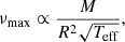
which are frequently used in inverted form to estimate stellar masses and radii from observed asteroseismic parameters (Stello et al. 2009; Kallinger et al. 2010):
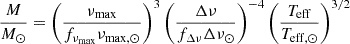
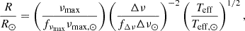
where fΔν and fνmax are correction factors. Since scaling relations were originally calibrated to the Sun, it is unsurprising that their validity in the red giant branch (RGB) phase has been questioned (e.g. Epstein & Pinsonneault 2014; Gaulme et al. 2016; Viani et al. 2017; Rodrigues et al. 2017; Zinn et al. 2019; Stello & Sharma 2022; Li et al. 2023). Correction factors have been investigated by many authors across different ranges of mass, metallicity, and evolutionary phase (e.g. White et al. 2011; Sharma et al. 2016; Rodrigues et al. 2017; Guggenberger et al. 2017; Stello & Sharma 2022; Li et al. 2022; Pinsonneault et al. 2018). At present, while it is possible to use stellar models and pulsation theory to investigate the correction factor fΔν, understanding of the excitation, damping, and reflection of modes is still insufficient to do the same for fνmax, although some efforts exist in the literature (e.g. Viani et al. 2017; Zhou et al. 2020, 2024). This issue is currently addressed by calibrating fνmax to observations (e.g. Li et al. 2022; Pinsonneault et al. 2025).
Concerning fΔν, a widespread approach to correcting scaling relations is to obtain theoretically motivated corrections to the observed Δν, to reconcile the observed large frequency spacing with the theoretical Δνs assumed in asymptotic pulsation theory (e.g. Sharma et al. 2016; Guggenberger et al. 2017; Stello & Sharma 2022). These corrections depend on the evolutionary state of the star, as well as its mass, temperature, surface gravity, and metallicity. Their evaluation requires computing a large grid of stellar models, calculating oscillation frequencies using a stellar oscillation code, determining the average large frequency spacing Δν0, and it with Δνs from scaling relations. In the following we adopt the definition

Including correction factors, estimated masses and radii show general agreement for stars in eclipsing binary systems (e.g. Brogaard et al. 2018; Hekker 2020, and references therein). Today, model-based corrections that account for stellar mass, evolutionary stage, and metallicity, such as those by Sharma et al. (2016), are widely adopted in asteroseismic-based Galactic archaeology studies (e.g. Yu et al. 2018; Zinn et al. 2019; Warfield et al. 2021; Wang et al. 2023; Schonhut-Stasik et al. 2024; Warfield et al. 2024; Valle et al. 2024). A potential issue in adopting masses and radii from corrected scaling relations is the existence of discrepancies between theoretical and observed oscillation frequencies in stars with solar-like oscillations. One example is the surface effect, which originates from improper modelling of the stellar surface layers. Correcting for this effect remains an ongoing process (Ball et al. 2018; Jørgensen et al. 2019; Li et al. 2023, and references therein). Another concern is the possible discrepancy between observed and theoretical temperatures for stars on the RGB (Martig et al. 2015; Valle et al. 2024). As shown by Gaulme et al. (2016), a difference of 100 K in effective temperature corresponds to differences of about 3% and 1%, in estimated masses and radii, respectively.
Beyond these practical challenges, a fundamental theoretical concern that impacts the accuracy of the fΔν correction factor is the inherent flexibility that stellar modellers have inconstructing the grids used to calculate these corrections. Specifically, the uncertainties in the input physics for stellar evolution codes introduce a significant degree of freedom in the selection of physical processes and parameters during model computation. Consequently, correction factors or calibrations derived from one set of stellar models cannot be reliably applied to models generated with different input physics. The dependence of the correction factor on stellar models has been explored in several studies (e.g. Pinsonneault et al. 2018; Li et al. 2023; Pinsonneault et al. 2025), revealing variations of a few percent due to differing model assumptions. However, these investigations overlook the intrinsic variability within the stellar models themselves. Given the limited research on this topic, the primary objective of this article is to systematically investigate this issue using a test case. We adopted the same methodological framework established by Sharma et al. (2016) but employed a different set of reference stellar models. In detail, we systematically varied seven key parameters, including initial chemical composition, evolutionary processes, and input physics, as outlined in Sect. 2. These variations were carefully chosen to represent a wide range of plausible choices in stellar modelling. For each reference model, we computed the fΔν factors throughout the RGB evolution. By directly comparing the results obtained under different reference scenarios and performing a statistical analysis of the impact of various parameters, we aim to shed light on the influence of stellar model uncertainties on the fΔν corrections.
2. Methods
2.1. Stellar models
Stellar models were computed with Modules for Experiments in Stellar Astrophysics (MESA) r24.03.01 for a 1.0 M⊙ star. The models evolved from the pre-main sequence up to the RGB until log g = 1.4 dex. These values were chosen to represent a typical star in the APO-K2 catalogue (Schonhut-Stasik et al. 2024), covering the RGB range spanned by the catalogue stars. Seven key parameters that impact stellar evolution and asteroseismic observables were varied dichotomously to represent different legitimate choices made by stellar modellers (see Table 1). Given the current theoretical and observational uncertainties, none of the options considered can be definitively considered more accurate or appropriate. All explored configurations were implemented using the standard MESA distribution, without the development of custom code.
Parameters varied in the stellar models computation and their corresponding values.
The first group of parameters concerned the initial chemical abundances. This included the reference solar mixture and the initial helium abundance. For the former, we adopted two widely used mixtures: the Grevesse & Sauval (1998) mixture (hereafter GS98) and the Asplund et al. (2009) mixture (hereafter AP09). For the latter, we set the initial helium abundance as Y = Yp + ΔY/ΔZ, where Yp = 0.2471 from Planck Collaboration VI (2020). The helium-to-metal enrichment ratio, ΔY/ΔZ, was set to 2.0 and 1.5, values consistent with the current uncertainty in this parameter (e.g. Tognelli et al. 2021, and references therein). The initial metallicity was fixed at [Fe/H] = −0.5, to match the median metallicity in the APO-K2 sample. This corresponds to Z = 0.00538 and 0.00540 for ΔY/ΔZ = 2.0 and 1.5, respectively, when adopting the GS98 solar mixture. The same values of Z were also adopted for the AP09 solar mixture. Stellar data fitting often uses the surface [Fe/H] to represent metallicity, and the correspondence between [Fe/H] and the total metallicity Z depends on the chosen reference solar mixture. Since a change of Z has a significant effect on stellar evolution, fixing [Fe/H] for model comparisons could introduce spurious differences. Therefore, we preferred to fix Z rather than [Fe/H] to avoid inflating the differences due to the mixture change.
The second group of parameters represented the inclusion of additional physical processes, specifically microscopic diffusion and mass loss. For microscopic diffusion, two extreme scenarios were considered. While microscopic diffusion has been shown to be efficient in the Sun (see e.g. Bahcall et al. 2001), its efficiency in Galactic globular cluster stars remains the subject of debate (see e.g. Korn et al. 2007; Gratton et al. 2011; Nordlander et al. 2012; Gruyters et al. 2014). Therefore, we computed a set of models accounting for gravitational settling, without radiative acceleration, following the standard MESA implementation (Paxton et al. 2018), and a set excluding it. For mass loss, the Reimers (1975) mass-loss formalism was adopted, with the η parameter ranging from 0.0 to 0.2. These values are consistent with those found in studies of open clusters (Miglio et al. 2012; Handberg et al. 2017).
The remaining parameters were related to the algorithmic computation of the stellar models. The opacity, κ, in the atmosphere was assumed to be either uniform throughout the atmosphere, with a value set by the outermost cell, or varied with depth using the MESA kap module at the local optical depth τ (Jermyn et al. 2023). The mixing-length parameter, αml, was fixed at the solar-calibrated value or decreased by 0.1 to model potential variations throughout stellar evolution (Magic et al. 2015). A solar calibration was performed for each set of model parameters. This was achieved by iteratively refining the metallicity Z, initial helium abundance Y, and mixing-length parameter using a Levenberg–Marquardt algorithm1. The calibration aimed to reproduce the observed solar radius, luminosity, logarithm of the effective temperature, and surface Z/X at the Sun’s current age. The iterative process terminated when the sum of the squared relative differences between the model outputs and the target values was less than 10−7. Mass loss was not included in this calibration process.
Finally, boundary conditions were set using either the solar-calibrated Hopf T(τ) relation (Paxton et al. 2013), a fit to Model C of the solar atmosphere by Vernazza et al. (1981), or the solar-calibrated Eddington T(τ) relation. While this parameter set does not encompass the full range of variability affecting models and pulsation frequencies, it includes many key factors that undoubtedly impact RGB evolution2.
2.2. Experiment design
To assess the importance of individual parameters, a full factorial design involving evaluation of all 27 combinations was deemed impractical due to inefficiency. In a computer experiment, where random variability between replicates is absent, an orthogonal array design – a generalisation of the Latin hypercube design – was more appropriate due to its higher efficiency (Art 1992; Hedayat et al. 1999). In an orthogonal array, each factor (i.e. each parameter in Table 1) appears with equal frequency at each level (i.e. each option in Table 1), and each pair of factors is included with the same frequency for each pair of levels. Therefore, in our experimental design, each pair of factors was considered an equal number of times for the four possible combinations of options. Since our primary goal was to assess the impact of individual parameters (i.e. main effects), rather than their interactions (which were assumed to be of minor relevance), an orthogonal design was appropriate.
Using the R library DoE.base (Grömping 2018), we generated a set of 32 random orthogonal combinations of the seven parameters. The design matrix used in the experiment is presented in Table 2, where each factor is coded as 0 or 1, with 0 indicating that Option 1 in Table 1 was adopted.
Design matrix of the 32 orthogonal combinations of the seven considered parameters.
2.3. Oscillation frequency computation
The oscillation frequencies were calculated using GYRE 7.1 (Townsend & Teitler 2013; Townsend et al. 2018) from stellar structure profiles computed with MESA. The structure of the stellar atmosphere was included in the stellar profiles. For each stellar track, oscillation frequencies were computed from log g = 3.2 to log g = 1.4 in steps of 0.01, following the RGB evolution. We adopted the approach of White et al. (2011) to derive Δν0 for each model, mimicking how this parameter is measured from the data (Sharma et al. 2016; Stello & Sharma 2022). The observed oscillation power spectrum of solar-like stars is characterised by a typical Gaussian-like envelope, peaked at νmax. To mimic the observable frequency ranges for each model, the frequencies were weighted based on their position within a Gaussian envelope centred at νmax, with a full width at half maximum given by  (Mosser et al. 2012; Bellinger et al. 2016). The frequency of maximum oscillation power was derived using the scaling relation, adopting the MESA default νmax, ⊙ = 3078 μHz from Lund et al. (2017). The value of Δν0 was then obtained by weighted regression of the oscillation frequencies versus their radial order.
Corresponding values of Δνs were obtained from the scaling relation, with MESA default Δν⊙ = 134.91 μHz from Lund et al. (2017). The ratio fΔν of the computed to scaling relation large frequency separation was then computed for each model, as described in Eq. (5).
3. Results
The trends of fΔν versus log g are shown in Fig. 1 for all 32 cases considered. The trend from Sharma et al. (2016) for Z = 0.00477 is also included as a reference3. The qualitative behaviour is consistent across all 32 considered cases and agrees with the results of Sharma et al. (2016) results. The most notable feature is the significant variability observed in fΔν. The maximum difference in the correction factor increases almost steadily from 0.013 to 0.030 as log g decreases from 3.2 to 1.4. Given the fourth-power dependence of the asteroseismic mass on fΔν, this variability leads to systematic differences in the masses estimated from the corrected scaling relations, ranging from about 5% to more than 10%. This range of difference in the correction factor depends only slightly on the stellar mass. In Appendix A we present the results for models with masses of 0.8 M⊙ and 1.2 M⊙, respectively. Their analysis confirms the robustness of the results presented here.
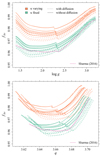 |
Fig. 1. Evolution of the fΔν ratio for the 32 parameter combinations considered. Top panel: trend of fΔν vs. log g. The solid violet line indicates the reference model with M = 1.0 M⊙, Z = 0.00477, based on the Sharma et al. (2016) data set. Different colours represent models with varying (orange) and fixed (green) opacity κ in the atmosphere, the primary source of systematic uncertainty in fΔν. Line styles differentiate models calculated with (dashed) and without (solid) microscopic diffusion, which is the second most significant contributor to systematic uncertainty in fΔν. Bottom panel: same as the top panel, but shown as a function of the q parameter. |
In practical applications of the fΔν correction, selecting the appropriate factor from a computed grid requires consideration of not only log g, but also effective temperature, mass, and metallicity. For instance, Sharma et al. (2016) and Stello & Sharma (2022) utilise an interpolating variable, q, that encapsulates the combined influence of effective temperature and log g:
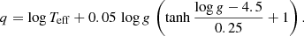
The bottom panel of Fig. 1 shows that the tracks cross at q ≤ 3.64, which corresponds to the terminal part of the RGB. As in the previous analysis, we found that the maximum difference in the correction factor increases almost steadily from 0.015 to 0.032 as q increases from 3.62 to 3.69. Since the tested cases represent reasonable and justifiable choices in stellar model computation, this variability poses a theoretical challenge when applying corrections to the scaling relations.
To investigate the origin of this variability, a linear model was fitted to describe the dependence of the correction factor on the stellar model parameters. To account for the non-linear dependence on log g, a dummy factor was included in the model to adjust for differences in the mean values of fΔν across the RGB points for each case. However, we found that excluding this stratification factor had a negligible impact on the estimated model parameters. The final model is given by:
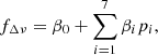
where β denoted the regression coefficients and pi are dichotomous categorical variables representing the two possible values of the i-th parameter in Table 1. The model coefficients are presented in Table 3. The most significant source of variability in the correction factor was the computation of opacity κ in the atmosphere. Using a variable κ in the stellar model computations increases fΔν by approximately 1.2% which is approximately one third to one half of the Sharma et al. (2016) correction. The second most important factor was the inclusion of microscopic diffusion, as stellar models that accounted for this process yielded a lower fΔν by about 0.4%. The other parameters had a lower impact, around 0.1% to 0.2%, with the exceptions of the helium-to-metal enrichment ratio and the inclusion of mass loss, which were found to be statistically insignificant. However, the importance of the helium-to-metal enrichment ratio may increase at higher initial metallicities due to the assumed link between Z and initial Y.
Coefficients and statistical significance from the linear model describing the dependence of fΔν on stellar model parameters.
4. Conclusions
We investigated the variability in the computation of the correction factor fΔν for the scaling relations. We adopted a framework identical to that of Sharma et al. (2016), which is widely used in the literature. For the test case of M = 1.0 M⊙, different stellar models were computed, differing in the choice of seven input parameters: the reference solar mixture, the initial helium abundance, the inclusion of microscopic diffusion, the inclusion of mass loss, the computation of the opacity κ in the atmosphere, the adopted mixing-length parameter value, and the boundary conditions. Each parameter was varied between two different options, each of them being a legitimate choice for stellar model computations.
By adopting an efficient orthogonal array design, we selected 32 combinations of these parameters, and for each, stellar tracks were evolved with MESA r24.03.01 up to log g = 1.4 in the RGB phase. For each track, the oscillation frequencies were calculated in the RGB phase with GYRE 7.1, and the large spacing Δν0 was computed as in White et al. (2011). Finally, the correction factor fΔν was calculated as the ratio of fΔν to the value of the uncorrected scaling relations.
The correction factor showed substantial variability across the 32 selected reference stellar models. The range of variability in fΔν was lower, approximately 1.3% in the lower RGB, and steadily increased to approximately 3% in log g = 1.4. This variability is significant, being close to corrections frequently adopted in the literature, such as that of Sharma et al. (2016), and would cause variations in corrected mass from 5% to 10% in the absence of recalibration, such as that discussed by Pinsonneault et al. (2025). The most important contribution to this variability was the modelling of the opacity κ in the stellar atmosphere (about 1.2%), followed by the inclusion of microscopic diffusion (about 0.4%).
The most recent Galactic archaeology studies (e.g. Zinn et al. 2019; Warfield et al. 2021; Wang et al. 2023; Schonhut-Stasik et al. 2024; Valle et al. 2024) adopt corrections similar to those discussed here. In this respect, the relevance of the variability in the correction factor is clear, because the random variability affecting mass estimates directly translates into variability in the derived stellar ages. In fact, the uncertainty that affects determinations of the effective temperature of RGB stars, both theoretical (e.g. Straniero & Chieffi 1991; Salaris & Cassisi 1996; Vandenberg et al. 1996) and observational (e.g. Hegedũs et al. 2023; Yu et al. 2023), has raised concerns about the direct use of this constraint in grid-based fitting (Martig et al. 2015; Warfield et al. 2021; Vincenzo et al. 2021). To address this issue, stellar model grids for RGB stars are usually interpolated using the asteroseismic mass as a constraint (Martig et al. 2015; Warfield et al. 2021, 2024) or the theoretical effective temperature corresponding to that mass and Δν (Valle et al. 2024). Given the dominant role of stellar mass in determining RGB stellar ages, the systematic uncertainty reported here raises questions about the accuracy attainable when estimating the age of RGB stars.
Although the model parameters tested are likely among the main sources of variability in the calculation of fΔν, they are not the only factors. Moreover, their influence may vary across different metallicity ranges and stellar masses. For example, in more massive stars, microscopic diffusion is expected to play a minor role due to shorter evolutionary timescales. Conversely, for these stars, convective core overshooting is expected to impact the systematic variability of the correction factor. Despite these limitations, the findings of this study highlight the importance of considering systematic variability in correction factors for scaling relations that rely on a stellar model reference scenario.
Implemented via the marqLevAlg R library (R Core Team 2024; Philipps et al. 2023).
The MESA inlists used in the computations are available at https://github.com/mattdell71/fdnu.
This is the Z value closest to our choice of Z = 0.00538. Minor differences arose considering Z = 0.00601, the next value available in the Sharma et al. (2016) grid.
Acknowledgments
G.V., P.G.P.M. and S.D. acknowledge INFN (Iniziativa specifica TAsP) and support from PRIN MIUR2022 Progetto “CHRONOS” (PI: S. Cassisi) finanziato dall’Unione Europea – Next Generation EU.
References
- Art, B. O. 1992, Statistica Sinica, 2, 439 [Google Scholar]
- Asplund, M., Grevesse, N., Sauval, A. J., & Scott, P. 2009, ARA&A, 47, 481 [NASA ADS] [CrossRef] [Google Scholar]
- Baglin, A., Auvergne, M., Barge, P., et al. 2009, in IAU Symposium, eds. F. Pont, D. Sasselov, M. J. Holman, 253, 71 [NASA ADS] [Google Scholar]
- Bahcall, J. N., Pinsonneault, M. H., & Basu, S. 2001, ApJ, 555, 990 [NASA ADS] [CrossRef] [Google Scholar]
- Ball, W. H., Themeßl, N., & Hekker, S. 2018, MNRAS, 478, 4697 [Google Scholar]
- Bellinger, E. P., Angelou, G. C., Hekker, S., et al. 2016, ApJ, 830, 31 [Google Scholar]
- Borucki, W. J., Koch, D., Basri, G., et al. 2010, Science, 327, 977 [Google Scholar]
- Brogaard, K., Hansen, C. J., Miglio, A., et al. 2018, MNRAS, 476, 3729 [Google Scholar]
- Chaplin, W. J., Houdek, G., Appourchaux, T., et al. 2008, A&A, 485, 813 [NASA ADS] [CrossRef] [EDP Sciences] [Google Scholar]
- Christensen-Dalsgaard, J. 2012, Astron. Nach., 333, 914 [Google Scholar]
- Epstein, C. R., & Pinsonneault, M. H. 2014, ApJ, 780, 159 [Google Scholar]
- Gaulme, P., McKeever, J., Jackiewicz, J., et al. 2016, ApJ, 832, 121 [NASA ADS] [CrossRef] [Google Scholar]
- Gratton, R. G., Johnson, C. I., Lucatello, S., D’Orazi, V., & Pilachowski, C. 2011, A&A, 534, A72 [NASA ADS] [CrossRef] [EDP Sciences] [Google Scholar]
- Grevesse, N., & Sauval, A. J. 1998, Space Sci. Rev., 85, 161 [Google Scholar]
- Grömping, U. 2018, J. Stat. Soft., 85, 1 [Google Scholar]
- Gruyters, P., Nordlander, T., & Korn, A. J. 2014, A&A, 567, A72 [NASA ADS] [CrossRef] [EDP Sciences] [Google Scholar]
- Guggenberger, E., Hekker, S., Angelou, G. C., Basu, S., & Bellinger, E. P. 2017, MNRAS, 470, 2069 [NASA ADS] [CrossRef] [Google Scholar]
- Handberg, R., Brogaard, K., Miglio, A., et al. 2017, MNRAS, 472, 979 [CrossRef] [Google Scholar]
- Hedayat, A., Sloane, N., & Stufken, J. 1999, Orthogonal Arrays: Theory and Applications, Springer Series in Statistics (New York: Springer) [CrossRef] [Google Scholar]
- Hegedũs, V., Mészáros, S., Jofré, P., et al. 2023, A&A, 670, A107 [NASA ADS] [CrossRef] [EDP Sciences] [Google Scholar]
- Hekker, S. 2020, Front. Astron. Space Sci., 7, 3 [NASA ADS] [CrossRef] [Google Scholar]
- Howell, S. B., Sobeck, C., Haas, M., et al. 2014, PASP, 126, 398 [Google Scholar]
- Jermyn, A. S., Bauer, E. B., Schwab, J., et al. 2023, ApJS, 265, 15 [NASA ADS] [CrossRef] [Google Scholar]
- Jørgensen, A. C. S., Weiss, A., Angelou, G., & Silva Aguirre, V. 2019, MNRAS, 484, 5551 [Google Scholar]
- Kallinger, T., Mosser, B., Hekker, S., et al. 2010, A&A, 522, A1 [NASA ADS] [CrossRef] [EDP Sciences] [Google Scholar]
- Kjeldsen, H., & Bedding, T. R. 1995, A&A, 293, 87 [NASA ADS] [Google Scholar]
- Korn, A. J., Grundahl, F., Richard, O., et al. 2007, ApJ, 671, 402 [NASA ADS] [CrossRef] [Google Scholar]
- Li, T., Li, Y., Bi, S., et al. 2022, ApJ, 927, 167 [NASA ADS] [CrossRef] [Google Scholar]
- Li, Y., Bedding, T. R., Stello, D., et al. 2023, MNRAS, 523, 916 [NASA ADS] [CrossRef] [Google Scholar]
- Lund, M. N., Silva Aguirre, V., Davies, G. R., et al. 2017, ApJ, 835, 172 [Google Scholar]
- Magic, Z., Weiss, A., & Asplund, M. 2015, A&A, 573, A89 [NASA ADS] [CrossRef] [EDP Sciences] [Google Scholar]
- Martig, M., Rix, H.-W., Silva Aguirre, V., et al. 2015, MNRAS, 451, 2230 [NASA ADS] [CrossRef] [Google Scholar]
- Miglio, A., Brogaard, K., Stello, D., et al. 2012, MNRAS, 419, 2077 [Google Scholar]
- Mosser, B., Elsworth, Y., Hekker, S., et al. 2012, A&A, 537, A30 [NASA ADS] [CrossRef] [EDP Sciences] [Google Scholar]
- Nordlander, T., Korn, A. J., Richard, O., & Lind, K. 2012, ApJ, 753, 48 [NASA ADS] [CrossRef] [Google Scholar]
- Paxton, B., Cantiello, M., Arras, P., et al. 2013, ApJS, 208, 4 [Google Scholar]
- Paxton, B., Schwab, J., Bauer, E. B., et al. 2018, ApJS, 234, 34 [NASA ADS] [CrossRef] [Google Scholar]
- Philipps, V., Proust-Lima, C., Prague, M., et al. 2023, marqLevAlg: A Parallelized General-Purpose Optimization Based on Marquardt-Levenberg Algorithm, r package version 2.0.8 [Google Scholar]
- Pinsonneault, M. H., Elsworth, Y. P., Tayar, J., et al. 2018, ApJS, 239, 32 [Google Scholar]
- Pinsonneault, M. H., Zinn, J. C., Tayar, J., et al. 2025, ApJS, 276, 69 [NASA ADS] [CrossRef] [Google Scholar]
- Planck Collaboration VI 2020, A&A, 641, A6 [NASA ADS] [CrossRef] [EDP Sciences] [Google Scholar]
- R Core Team 2024, R: A Language and Environment for StatisticalComputing, R Foundation for Statistical Computing, Vienna, Austria [Google Scholar]
- Reimers, D. 1975, Memoires of the Societe Royale des Sciences de Liege, 8, 369 [Google Scholar]
- Ricker, G. R., Winn, J. N., Vanderspek, R., et al. 2015, J. Astron. Telesc. Instrum. Syst., 1, 014003 [Google Scholar]
- Rodrigues, T. S., Bossini, D., Miglio, A., et al. 2017, MNRAS, 467, 1433 [NASA ADS] [Google Scholar]
- Salaris, M., & Cassisi, S. 1996, A&A, 305, 858 [NASA ADS] [Google Scholar]
- Schonhut-Stasik, J., Zinn, J. C., Stassun, K. G., et al. 2024, AJ, 167, 50 [NASA ADS] [CrossRef] [Google Scholar]
- Sharma, S., Stello, D., Bland-Hawthorn, J., Huber, D., & Bedding, T. R. 2016, ApJ, 822, 15 [Google Scholar]
- Stello, D., & Sharma, S. 2022, Res. Notes Am. Astron. Soc., 6, 168 [Google Scholar]
- Stello, D., Chaplin, W. J., Bruntt, H., et al. 2009, ApJ, 700, 1589 [NASA ADS] [CrossRef] [Google Scholar]
- Straniero, O., & Chieffi, A. 1991, ApJS, 76, 525 [NASA ADS] [CrossRef] [Google Scholar]
- Tognelli, E., Dell’Omodarme, M., Valle, G., Prada Moroni, P. G., & Degl’Innocenti, S. 2021, MNRAS, 501, 383 [Google Scholar]
- Townsend, R. H. D., & Teitler, S. A. 2013, MNRAS, 435, 3406 [Google Scholar]
- Townsend, R. H. D., Goldstein, J., & Zweibel, E. G. 2018, MNRAS, 475, 879 [Google Scholar]
- Ulrich, R. K. 1986, ApJ, 306, L37 [Google Scholar]
- Valle, G., Dell’Omodarme, M., Prada Moroni, P. G., & Degl’Innocenti, S. 2024, A&A, 690, A323 [NASA ADS] [CrossRef] [EDP Sciences] [Google Scholar]
- Vandenberg, D. A., Bolte, M., & Stetson, P. B. 1996, ARA&A, 34, 461 [NASA ADS] [CrossRef] [Google Scholar]
- Vernazza, J. E., Avrett, E. H., & Loeser, R. 1981, ApJS, 45, 635 [Google Scholar]
- Viani, L. S., Basu, S., Chaplin, W. J., Davies, G. R., & Elsworth, Y. 2017, ApJ, 843, 11 [NASA ADS] [CrossRef] [Google Scholar]
- Vincenzo, F., Weinberg, D. H., Montalbán, J., et al. 2021, ArXiv e-prints [arXiv:2106.03912] [Google Scholar]
- Wang, C., Huang, Y., Zhou, Y., & Zhang, H. 2023, A&A, 675, A26 [NASA ADS] [CrossRef] [EDP Sciences] [Google Scholar]
- Warfield, J. T., Zinn, J. C., Pinsonneault, M. H., et al. 2021, AJ, 161, 100 [NASA ADS] [CrossRef] [Google Scholar]
- Warfield, J. T., Zinn, J. C., Schonhut-Stasik, J., et al. 2024, AJ, 167, 208 [NASA ADS] [CrossRef] [Google Scholar]
- White, T. R., Bedding, T. R., Stello, D., et al. 2011, ApJ, 743, 161 [Google Scholar]
- Yu, J., Huber, D., Bedding, T. R., et al. 2018, ApJS, 236, 42 [NASA ADS] [CrossRef] [Google Scholar]
- Yu, J., Khanna, S., Themessl, N., et al. 2023, ApJS, 264, 41 [NASA ADS] [CrossRef] [Google Scholar]
- Zhou, Y., Asplund, M., Collet, R., & Joyce, M. 2020, MNRAS, 495, 4904 [CrossRef] [Google Scholar]
- Zhou, Y., Christensen-Dalsgaard, J., Asplund, M., et al. 2024, ApJ, 962, 118 [Google Scholar]
- Zinn, J. C., Pinsonneault, M. H., Huber, D., et al. 2019, ApJ, 885, 166 [Google Scholar]
Appendix A: Mass dependence
This section compares the correction factors fΔν for stellar models with masses 0.8 M⊙ and 1.2 M⊙. As illustrated in Fig. A.1, the variation in fΔν due to input physics is nearly identical to that observed for the 1.0 M⊙ model, discussed in the main text.
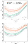 |
Fig. A.1. Evolution of the fΔν ratio with log g for the 32 parameter combinations considered. (Top): models computed with M = 0.8 M⊙. The colour and line codes are the same as in Fig. 1. (Bottom): same as in the top panel, but for M = 1.2 M⊙. |
All Tables
Parameters varied in the stellar models computation and their corresponding values.
Design matrix of the 32 orthogonal combinations of the seven considered parameters.
Coefficients and statistical significance from the linear model describing the dependence of fΔν on stellar model parameters.
All Figures
|
Fig. 1. Evolution of the fΔν ratio for the 32 parameter combinations considered. Top panel: trend of fΔν vs. log g. The solid violet line indicates the reference model with M = 1.0 M⊙, Z = 0.00477, based on the Sharma et al. (2016) data set. Different colours represent models with varying (orange) and fixed (green) opacity κ in the atmosphere, the primary source of systematic uncertainty in fΔν. Line styles differentiate models calculated with (dashed) and without (solid) microscopic diffusion, which is the second most significant contributor to systematic uncertainty in fΔν. Bottom panel: same as the top panel, but shown as a function of the q parameter. |
| In the text | |
|
Fig. A.1. Evolution of the fΔν ratio with log g for the 32 parameter combinations considered. (Top): models computed with M = 0.8 M⊙. The colour and line codes are the same as in Fig. 1. (Bottom): same as in the top panel, but for M = 1.2 M⊙. |
| In the text | |
Current usage metrics show cumulative count of Article Views (full-text article views including HTML views, PDF and ePub downloads, according to the available data) and Abstracts Views on Vision4Press platform.
Data correspond to usage on the plateform after 2015. The current usage metrics is available 48-96 hours after online publication and is updated daily on week days.
Initial download of the metrics may take a while.