| Issue |
A&A
Volume 690, October 2024
|
|
|---|---|---|
| Article Number | A340 | |
| Number of page(s) | 13 | |
| Section | The Sun and the Heliosphere | |
| DOI | https://doi.org/10.1051/0004-6361/202451375 | |
| Published online | 23 October 2024 | |
Density-dependent ionization equilibria for carbon with kappa distributions
1
Astronomical Institute of the Czech Academy of Sciences, Fričova 298, Ondřejov, Czech Republic
2
DAMTP, University of Cambridge, Wilberforce Road, Cambridge CB3 0WA, UK
Received:
4
July
2024
Accepted:
13
September
2024
Context. Recent atomic models for the solar transition region have shown the importance of electron density, photoionization, and charge transfer on the ionization equilibria and line intensities of several elements and ions, especially from the Li- and Na-like ion sequences.
Aims. Non-Maxwellian electron distributions have been proposed as one solution that may account for the discrepancies. We have studied the interplay of the new atomic models with the effects of energetic particles, which have been shown to alter ionization equilibria considerably.
Methods. Level-resolved ionization and recombination rates were calculated for non-Maxwellian kappa distributions and included in a collisional-radiative model for carbon. The effect of photoionization and density suppression of dielectronic recombination for kappa distributions were also included in the models, and the models were run at a variety of densities and pressures.
Results. We find that the level-resolved collisional ionization rates increase with electron density, while the radiative and dielectronic recombination rates decrease. Their overall effect on the ionization equilibrium is to shift the formation of the lower charge states to a lower temperature and increase their peak abundance, especially for C IV. These shifts are not as significant as the effects of the non-extensive shape parameter given by the thermodynamic kappa index, κ. With decreasing κ; that is, with increasing departure from a Maxwellian distribution, ion formation moves to a much lower temperature, ion formation takes place over a wider temperature range, and peak abundances decrease. The effect of level-resolved rates and density suppression on the ion balances diminishes as κ decreases. Photoionization is shown to be significant only at relatively low densities and high κ.
Conclusions. Density effects are an important factor to consider in higher-density plasma and improve on the coronal approximation, even where there are significant departures from Maxwellian energy distributions. However, the changes they make to ion formation are not as significant as when there are electron distributions with very low κ-values.
Key words: atomic processes / Sun: transition region
© The Authors 2024
 Open Access article, published by EDP Sciences, under the terms of the Creative Commons Attribution License (https://creativecommons.org/licenses/by/4.0), which permits unrestricted use, distribution, and reproduction in any medium, provided the original work is properly cited.
This article is published in open access under the Subscribe to Open model. Subscribe to A&A to support open access publication.
1. Introduction
It has long been known that some solar transition region lines have intensities that are strongly discrepant with both line intensities of other isoelectronic sequences, if the coronal approximation is employed. For example, lines of Li-like and Na-like ions, such as C IV and Si IV, have been observed with intensities a factor of ≈5 higher (Doyle & Raymond 1984; Hayes & Shine 1987; Judge et al. 1995; Curdt et al. 2001; Doschek & Mariska 2001; Del Zanna et al. 2002; Peter et al. 2014; Doschek et al. 2016; Polito et al. 2016; Dudík et al. 2017; Del Zanna & Mason 2018; Dufresne et al. 2023). The coronal approximation assumes that the ionization and recombination timescales are much longer than the timescales for excitation and de-excitation (see, e.g., Chapter 4.5 of Phillips et al. 2008). Consequently, the ionization and recombination processes and the calculation of the relative ion abundances (charge state) can be treated separately from the relative populations of excited levels. This means that the relative ion abundances are independent of electron density and that they can be tabulated (see, e.g., Jordan 1969; Arnaud & Rothenflug 1985; Mazzotta et al. 1998; Dere et al. 2023). In addition, the coronal approximation assumes that ionization and recombination happen between ground states of neighbouring ions.
A variety of processes have been found to affect the formation of transition region lines and thus their intensities, especially from Li-like and Na-like ions, including the electron density effects related to metastable excitation levels (Nussbaumer & Storey 1975; Doyle et al. 2005; Dufresne & Del Zanna 2019), photo-induced processes (Nussbaumer & Storey 1975; Dufresne et al. 2021a), resonant scattering and opacity (Doschek et al. 1991; Gontikakis et al. 2013), mixing of structures with different temperatures and densities at small spatial scales (Doschek & Feldman 1978; Doschek 1984), transient (time-dependent) ionization (e.g., Spadaro et al. 1994; Bradshaw et al. 2004; Olluri et al. 2013), and presence of high-energy electrons (Pinfield et al. 1999; Dzifčáková & Kulinová 2011; Dudík et al. 2014, 2017).
Although any and all of these processes can contribute to line formation depending on the situation, the effects of electron density, including suppression of dielectronic recombination (DR), ionization, and recombination from/to excited levels are always present and influence the formation of lines in the solar transition region. A series of works (Dufresne & Del Zanna 2019), Dufresne et al. (2020, 2021a,b) evaluated the effects of electron density on the intensities of solar transition region lines, concluding that their inclusion significantly increases the agreement with observed line intensities in quiet Sun (Dufresne et al. 2023). Updated charge transfer rates were also included. This modelling effort recently culminated with the inclusion of these effects in the CHIANTI database, version 11 (Dufresne et al. 2024).
Despite the significant improvements introduced by these atomic models, Dufresne et al. (2023) still found the Li- and Na-like line intensities to be under-predicted by factors of two to four compared with averaged, quiet Sun observations. One of the previously proposed explanations for the discrepant line intensities produced by Li-like and Na-like ions invoked the presence of accelerated particles (Pinfield et al. 1999; Dzifčáková & Kulinová 2011). These line intensities are strongly sensitive to the high-energy tail of the distribution because the presence of high-energy particles leads to changes of level populations and to strong increases of the ionization rates, especially at the relatively low temperatures of the transition region (see Dzifčáková 1992; Dzifčáková & Dudík 2013). A review by Del Zanna et al. (2015) found, however, that conclusive evidence from Si III observations was not present. On the other hand, accelerated particles in the solar transition region are expected to be present, especially along temperature- and density-stratified structures, where the more energetic particles from hotter upper parts of the atmosphere intrude into lower altitudes (Roussel-Dupré 1980; Shoub 1983; Ljepojevic & MacNeice 1988; Vocks et al. 2016). This is aided by the fact that the high-energy charged particles are progressively less collisional, as their collision frequency scales with energy as ∼E−3/2. Even a relatively small amount of charged particles can cause significant departures of line intensities from the equilibrium Maxwellian situation. Dzifčáková et al. (2017) have shown that a high-energy tail containing only 4% of particles (which carry about 25% of kinetic energy) can change the intensities of Si IV lines by a factor of two, and shift the formation of these lines to much lower temperatures.
Given how more advanced atomic models and non-Maxwellian electron distributions can alter line formation, this paper takes the first step in studying the interplay of both effects on the formation of line intensities in the solar transition region. It builds upon the collisional-radiative (CR) model of Dufresne & Del Zanna (2019) for carbon by calculating excitation, ionization, and recombination rates for electron kappa distributions, and includes them in a similar CR model. The focus of the present work is the ion fractions resulting from the model. This is a first step in building CR modelling of the transition region including kappa distributions.
The next Sect. 2 of this article describes the methods and data used to construct the models. This is followed in Sect. 3 by the presentation of the ion balances as each of the atomic processes are added to the models, namely ionization and recombination from metastable levels, photoionization, and suppression of DR, as well as the final model with all of the effects added together. The main conclusions are given in Sect. 4.
2. Methods
As mentioned, the ionization equilibrium in the coronal approximation was calculated as a density independent problem. This assumed that ionization and recombination from the ground levels dominates because excited levels have much lower populations in comparison. However, this is not valid in plasma where densities are high enough that there is a significant population of ions in excited levels. These so-called metastable levels usually have ionization rates that are higher than those of the ground. This results in higher overall ionization rates out of the ion. Conversely, the recombination rates are often lower than those of the ground, also affecting the overall recombination rate out of the ion. Dielectronic recombination for electron densities and temperatures typical for the transition region takes place through the highly excited levels. Recombined ions in these states are rapidly reionized by electron collisions, leading to DR suppression. Clearly, these effects alter the way ions form in such conditions relative to models which only include ionization and recombination from ground levels.
Dufresne & Del Zanna (2019) presented a CR model for carbon which includes the above density effects, as well as photoionization. They used the latest atomic data, and the model was run in ionization equilibrium to assess how line emission in the solar transition region was altered relative to the coronal approximation. From this first work, they built a database of atomic data and codes which includes density effects, radiative processes, and charge transfer for a total of seven elements. In the present work, we used the same data and methods as Dufresne & Del Zanna (2019) to build a CR model for carbon, but we included rates using non-Maxwellian electron distributions to assess the balance of electron distribution and density effects. In doing so, we omitted charge transfer because it does not affect the ionization balance of carbon in the solar atmosphere (Dufresne et al. 2021a).
2.1. Non-Maxwellian electron kappa distributions
Here, we characterize the electron distributions by the well-known kappa distributions, a family of non-Maxwellian distributions with enhanced number of particles in the high-energy tail described by the thermodynamic index κ (e.g., Vasyliunas 1968a,b; Olbert 1968; Owocki & Scudder 1983; Livadiotis 2017; Lazar & Fichtner 2021). These kappa distributions are the most generalized version of the classical Maxwell-Boltzmann (MB) distributions which are consistent with thermodynamics. They describe the particle energies in systems with correlations among their particles, such as space plasma, where the particle correlations are induced by long-range interactions or turbulence (see, e.g., Hasegawa et al. 1985; Laming & Lepri 2007; Bian et al. 2014; Livadiotis & McComas 2009; Livadiotis 2017). The kappa distributions are characterized by the thermodynamic parameter (index) kappa, κ, while they recover the MB distributions at the limit of κ → ∞:
In this equation, T is the temperature, kB is the Boltzmann constant, and Aκ = Γ(κ + 1)/((κ − 3/2)3/2Γ(κ − 1/2)) is the normalization constant, approaching 1 as κ → ∞. The properties and use of kappa distributions for spectral synthesis are described in Dzifčáková et al. (2015, 2021, 2023).
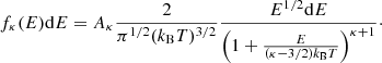
To aid understanding of the results shown throughout this work, example electron distributions are illustrated in Fig. 1. Three different cases are highlighted: Case (1) shows that kappa distributions have a high-energy tail, where the number of particles is far greater than in a Maxwellian distribution. At intermediate energies labelled as Case (2), this is reversed, as the number of particles is lower in a κ-distribution than in a Maxwellian. Finally, Case (3) is the low energy regime, where kappa distributions have a higher number of particles present.
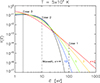 |
Fig. 1. Comparison of the Maxwellian distribution with kappa distributions for κ = 10, 5, 3, and 2, at Temperature 5 × 10⁴ K. The different colours correspond to different distributions. |
2.2. Level populations
Only ground and metastable levels of carbon ions were assumed in our calculations of level-resolved ionization and recombination rates. The initial levels for ionization and recombination are listed in Table 1. For C V and C VI, which do not have mestastable levels, only the ionization and recombination from ground level were calculated. Level populations of carbon ions were calculated using the KAPPA package (Dzifčáková et al. 2015, 2023) for kappa distributions with κ = 2–33 and for Maxwellian distribution. Electron densities were taken in the range log(ne [cm−3]) = 7–13.
Excitation levels for which the individual ionization and recombination rates were calculated.
Figures 2 and 3 show the calculated relative level populations of C II (left) and C III (right). Changes in level populations occur with changing electron density (Fig. 2). Nevertheless, the level populations are also dependent on T and κ (Fig. 3). At log(T [K]) ≈ 4.0, metastable level populations for small values of κ are greater than for Maxwellian electron distributions. This corresponds to the Case 3 region highlighted in Fig. 1, in which scenario more non-Maxwellian electrons are present to excite ions into metastable levels. However, for temperatures above log(T [K]) ≈ 4.3, corresponding to the Case 2 region, metastable level populations decrease as κ becomes smaller. This behaviour persists until about log(T [K]) ≈ 5.5, when the metastable level populations are again higher for low κ values. This behaviour reflects changes in the excitation rates with κ. Of course, details depend on the excitation energy and transition parameters.
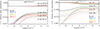 |
Fig. 2. Level populations in C II (left) and C III (right) plotted as a function of electron density log(ne [cm−3]). The temperature is indicated. The different colours correspond to different distributions. |
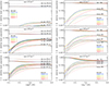 |
Fig. 3. Level populations in C II (left) and C III (right) plotted as a function of temperature log(T [K]) at three different densities, log(ne [cm−3]) = 7, 9, and 11. The different colours correspond to different distributions. |
2.3. Ionization rates
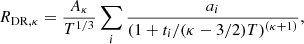
The level-resolved cross-sections for direct ionization (DI) and excitation-autoionization (EA, or indirect ionization) were taken from Dufresne & Del Zanna (2019). Rates were calculated by direct numerical integration over kappa distributions, R = ∫σvf(E)dE, where σ is cross-section and v is electron velocity. The total rate from each initial metastable level (Table 1) was obtained as a sum of ionization rates from this level to all final levels in the next higher charge state.
Figure 4 shows how the overall direct ionization and excitation-autoionization rates out of C II and C III change when plasma density and electron distribution change. Three different electron densities, log(ne [cm−3]) = 7, 9, and 11 were chosen to illustrate the dependence of these rates on ne. For these ions, the ionization rates for kappa distributions are several orders higher than for Maxwellian distribution for temperatures lower than log(T [K]) ≈ 4.5 for C II and log(T [K]) ≈ 5.0 for C III. This region corresponds to the Case 3 region of the electron distribution shown in Fig. 1. As electron density increases so do the direct ionization and excitation-autoionization rates, because the metastable levels are becoming more populated with increasing electron density (see Fig. 2). The magnitude of this effect for higher temperatures in some cases can be comparable with the effect of distributions on the ionization rates (see the bottom right panel of Fig. 4). Clearly, the effect with electron density is stronger for C III because its metastable levels have higher populations than C II.
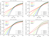 |
Fig. 4. Dependence of the direct ionization (top panels) and excitation-autoionization rates (bottom panels) from C II → C III (left) and C III → C IV (right) at three different electron densities, log(ne [cm−3]) = 7, 9, and 11. The different colours correspond to different distributions, as indicated. The bottom right panel only shows the autoionization rate for κ = 2, 5, and Maxwellian for increased clarity (κ = 3 and 10 are omitted). |
2.4. Recombination rates
The same recombination data used by Dufresne & Del Zanna (2019) for rates from initial ground and metastable levels were used here. The radiative recombination (RR) rates were from Badnell (2006) and the DR data were from Badnell et al. (2003) and later works in the series. Total rates from each initial level summed over all final states were used from those works.
For the calculation of RR rates for kappa distributions, we used a technique described in Dzifčáková (1992) and Dzifčáková & Dudík (2013). According to (Osterbrock 1974) it is assumed that the cross-section varies as a power law in energy, σRR(E) = CRREη + 0.5, where CRR is a constant and η + 0.5 is a power-law index. The RR rate for a Maxwellian distribution then is
and for kappa distributions it is
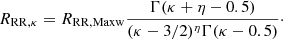
Examples of the behaviour of the RR rates for C II and C III are shown in the top panels of Fig. 5. The most important characteristic is a strong increase of RR rates with decreasing κ (a factor 2 or 3 for κ = 2), caused by a relatively larger number of low-energy electrons in a κ-distribution (Case 3, see also Dzifčáková & Dudík 2013). There is a small decrease in the RR rates as the metastable levels become populated with increasing ne because the recombination rates from metastable levels are lower than those from the ground. However, it can be seen that the effect of finite electron densities on the overall RR rates is much smaller than the effect of electron distribution.
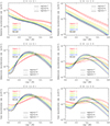 |
Fig. 5. Effect of metastable levels on the radiative (top), dielectronic (middle), and total recombination rates (bottom) for the recombination from C II → C I (left) and C III → C II (right), for three different electron densities, log(ne [cm−3]) = 7, 9, and 11, as indicated. The different colours correspond to different distributions. |
For the DR rate, RDR, κ, we used the approximation derived by Dzifčáková (1992),
where parameters ai and ti are t he same as in similar expressions for the Maxwellian distribution.
The influence of kappa distributions on DR rates for C II and C III is shown in the middle panels of Fig. 5. The maxima of the RDR, κ can be shifted to higher temperatures, and the maxima are both lower and wider. For some ions, such as C III, the changes in the DR rate with electron densities for the case of extremely low κ = 2 can be more pronounced than the changes in the RR rates (compare the top and middle panels of Fig. 5). This and the higher RR rates associated with non-Maxwellian electrons lead to an increase in the relative importance of RR, especially at low temperatures. This effect does not necessarily apply for all ions, but depends on the atomic data in each case.
The changes seen in the DR rates as electron density varies are similar whether there are κ or Maxwellian distributions. The increase in the rates with temperature is caused by the increase in the populations of the metastable levels. Again, it is the C III rates that are more affected by density because its metastable levels have a higher fractional population than those in C II.
2.5. Estimation of density suppression of DR
In finite-density plasma, DR rates are suppressed with respect to the process in a low-density plasma (see Burgess & Summers 1969; Summers 1972, 1974; Summers & Hooper 1983; Badnell et al. 1993, 2003). DR is a multi-step process which occurs when an incoming, free electron captured by an ion excites one of the bound electrons, producing a doubly excited resonance state. Various channels are then available, but if the recombined ion stabilizes to a bound state through radiative decay of the core or Rydberg electron, then the DR process is complete. Such an ion left in a Rydberg state is susceptible to being reionized through collisions with a free electron, particularly in higher-density plasma. Burgess & Summers (1969) showed that this effect could occur already in coronal densities of log(ne [cm−3]) = 8, and is thus even more significant in the cooler lower atmosphere. Modelling the effect self-consistently is complex as it requires rates connecting all of the different channels and atomic processes, potentially for hundreds of levels.
Consequently, there have been several attempts to approximate the effect. Nikolić et al. (2013) developed a general model to calculate the density-dependent DR rate for Maxwellian distribution. These authors have shown that the density suppressed DR rate RDR(ne, T, q, M) can be expressed as

where RDR(T) is the DR rate in zero density limit. The suppression factor (SF), S(ne, T, q, M), is dimensionless and depends on the electron density ne, temperature T, and isoelectronic sequence M, as well as the parameter q which depends on the ion. Nikolić et al. (2018) provided improved fits to the SFs at intermediate densities for a Maxwellian distribution. They are used within CHIANTI v.11.
This approach was adapted to kappa distributions by Dzifčáková et al. (2023), who estimated density suppression of DR rates for kappa distributions as
where aj are the coefficients of the approximation of a κ-distribution by a sum of several Maxwellians at different temperatures Tj (see Hahn & Savin 2015). This approximation of suppression of DR rate for kappa distributions was used in our calculation of density dependent ionization equilibria for kappa distributions. Appendix A presents details on the use and precision of this Maxwellian decomposition method.
2.6. Photoionization rates
Photoionization is also an important atomic process when modelling the low charge states of carbon (Nussbaumer & Storey 1975). The photoionization rate is given by the expression (see, e.g., Nussbaumer & Storey 1975; Dufresne & Del Zanna 2019; Dufresne et al. 2021a)
where σphot is the ionization cross-section, Jλ is the mean intensity, λ is the wavelength, h is Planck constant, and c is speed of light. We used the same cross-sections and mean intensities as in the Dufresne & Del Zanna (2019) models. Namely, the cross-sections are from Badnell (2006), and the mean disk intensity was obtained from the solar minimum irradiances of Woods et al. (2009), assuming no limb brightening.
We note that the Rphot depends on the ambient radiation field and is independent of κ. The Rphot, however, does depend on the distance r above the solar surface through the dependence of Jν on the dilution factor, W(r), where Jλ =  . Here,
  is the average disk radiance at wavelength λ. The above radiances are clearly too low if one is interested in modelling, for instance, an active region. However, the treatment here is sufficient to assess the relevance of this process in the presence of alternative electron distributions. Finally, Dufresne & Del Zanna (2019) also investigated photoexcitation and found that it had no bearing on carbon ion fractions.
3. Ionization Equilibrium
3.1. Ionization equilibria with level-resolved rates
As electron density is a parameter directly related to the population of metastable levels, we first investigated the various effects related to electron density on the ionization equilibria.
The ionization equilibria including the effect of level-resolved ionization and recombination rates for kappa distributions with κ = 2, 5, 10, and Maxwellian distribution for electron densities of log(ne [cm−3]) = 7, 9, and 11, are shown in Fig. 6. It can be seen that the main changes in the carbon ion abundances with electron density are in the temperature range below log(T [K]) = 5.2. For Maxwellian and high κ distributions the ionization peaks are slightly shifted to lower temperatures with increasing electron densities. However, more significant changes to the ion fractions occur with the electron distribution, as the peaks are widened and shifted to lower temperatures as κ decreases (Dzifčáková & Dudík 2013). For low values of κ as electron density varies, there is clearly a much smaller effect on the relative ion abundances.
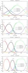 |
Fig. 6. Carbon ionization equilibria including only ionization and recombination from/to excited levels, i.e., without DR suppression or photoionization, calculated for Log(ne/cm−3) = 7 (full lines), 9 (dashed lines), and 11 (dot-dashed lines), and for kappa distributions with κ = 2, 5, 10, and Maxwellian distribution. The different colours correspond to different ions. |
This effect can be understood from the ionization and recombination rates discussed in Sect. 2. The ionization rates are orders of magnitudes faster at low temperatures relative to Maxwellian distributions (Fig. 4). However, recombination rates only increase by a factor of two (Fig. 5), and so the overall effect is to cause the ions to form much lower in the atmosphere. At these low temperatures the populations of the metastable levels are not strongly changed when density increases (Fig. 2). This then leads to minimal changes in the ion balances for low κ as pressure varies.
For all cases, the most important change is the increase of the abundance maximum for C IV, which occurs for both increasing electron density as well as decreasing κ. For a Maxwellian distribution, the maximum of C IV abundance increases by about a factor of 1.25 with electron density changing from log(ne [cm−3]) = 7 to 11. However, for the κ-distribution with κ = 2, its increase in peak abundance becomes almost negligible as electron density changes over this range, although in its peak, the maximum of the C IV ion abundance at log(ne [cm−3]) = 11 is comparable (≈0.4) to that in the Maxwellian ion balance (see Table 2).
Maximum abundance of C IV as a function of ne and κ in ionization equilibrium including resolved ionization and recombination only.
3.2. Ionization equilibrium with photoionization
The changes caused by adding photoionization to the level-resolved ionization equilibria are shown in Fig. 7 for three model cases, κ = 2, 5, and 10. It is seen that photoionization is significant at low electron densities (log(ne [cm−3]) = 7) and higher values of κ, where it dominates. For such cases, it leads to strong changes in the shape of the ionization peaks of C I–C IV at temperatures below 105 K (bottom panel of Fig. 7). At these temperatures, C I is almost nonexistent, (i.e. it is fully ionized), while the abundance of C II decreases by about an order of magnitude. Contrary to that, the C III and C IV are abundant at any temperature between 104–105 K. The ion C V, which forms above log(T [K]) = 5.5, as well as higher charge states are not affected because solar emission at such high ionization energies is much weaker.
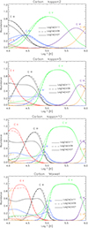 |
Fig. 7. Level-resolved Carbon ionization equilibria including photoionization for quiet Sun without DR suppression shown for different log(ne [cm−3]) and κ = 2, 5, 10, and for Maxwellian distributions. The different colours correspond to different ions. |
For higher electron densities of log(ne [cm−3]) ≥ 9, the effect of photoionization decreases sharply, by a factor of more than 100, and the ionization peaks almost are not influenced. Thus, photoionization would be an important factor on the ion balances if there are pockets of low-density plasma in the atmosphere. Higher charge states than expected would be present compared to a collisional plasma, although line emission from such regions might be too low compared to neighbouring, high-density regions to be able to detect this.
For κ-distribution with low values of κ, such as κ = 2, the effect of photoionization on the ionization peaks is small (top panel of Fig. 7). In this case, the electron collisional ionization is several orders higher than, for example, for κ = 10 (Fig. 4), meaning that the collisional ionization rate becomes much stronger than the photoionization rate for such small values of κ, suppressing the effects of photoionization on the total ionization rate even at low electron densities.
3.3. Ionization equilibrium with density suppression of DR
As mentioned earlier, suppression of DR in finite-density plasma is an important effect on the ionization equilibrium, one that can increase with increasing electron density (c.f., Dufresne & Del Zanna 2019 and one that exists even for the non-Maxwellian kappa distributions (Dzifčáková et al. 2023), although details depend on the given element and ion. Here, its importance for carbon is studied in the Appendix B. Figure B.1 shows the changes in the carbon ion abundances, calculated including level-resolved ionization, recombination, and density suppression of DR. The changes are plotted as a ratio of ion abundances calculated including DR suppression with respect to it being omitted.
It is found that with decreasing κ, DR suppression is generally diminished, and its effect on the resulting ionization equilibrium becomes less pronounced. This diminishing of DR suppression with decreasing κ occurs because the ion formation takes place at lower temperatures. At lower temperatures the collisional ionization rates, which suppress the recombination process into highly excited levels, are weaker. Also, as discussed in Sect. 2, RR contributes more to the total recombination rate at these temperatures, reducing the influence of DR suppression.
The maximum relative ion abundances of C IV and their changes with κ with inclusion of DR suppression are presented in Table 3. Increasing electron density results in the increase of the relative C IV ion abundance. For lower κ, the increase becomes progressively less pronounced compared to Maxwellian distribution.
Maximum abundance of C IV as a function of ne and κ in ionization equilibrium including resolved ionization and recombination, as well as density suppression of DR.
3.4. Final ionization equilibrium for constant pressure
The assumption of constant pressure is usually employed when calculating the emission from the solar transition region, where both temperatures and densities change along a single structure on short spatial scales. Therefore, we calculated the ionization equilibria for carbon at constant pressures of p = T × ne = 1014, 1015, and 1016 K cm−3, and included the effects of level-resolved ionization and recombination, DR suppression, and photoionization. The results are shown in Fig. 8. These equilibria cover real physical parameters in the transition region, such as coronal holes, the quiet Sun, and active regions, and better show possible changes in carbon ion abundances due to electron density.
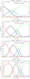 |
Fig. 8. Carbon ionization equilibria with ionization and recombination from density-dependent metastable states, DR suppression and photoionization for quiet Sun at constant pressures p = 1014(full lines), 1015 (dot-dashed), and 1016 K cm−3 (dashed) shown for κ = 2, 5, 10, and Maxwellian distributions. The thin dotted lines correspond to the ionization equilibrium using the coronal approximation, that is, without level-resolved ionization, recombination, DR suppression, and photoionization. |
For comparison, the thin dotted lines in Fig. 8 show the ionization equilibrium without level-resolved ionization, recombination, DR suppression, and photoionization, that is, the coronal approximation. Our ionization equilibria with density-induced effects show strong changes to the ionization equilibria compared to the coronal approximation. Including the density effects (level-resolved ionization and recombination and DR suppression) shifts the ionization equilibria to lower temperatures regardless of the type of distribution. The highest shift is for the κ = 2 distribution (Δlog(T) ≈ 0.25), and the the smallest is for Maxwellian distribution (Δlog(T) ≈ 0.15).
For a Maxwellian distribution and high κ ( = 10, the lower two panels of Fig. 8), the changes with pressure are the most pronounced. Firstly, the shift in the ion peaks and formation temperature when all the processes are added are more significant here than for lower κ. At p = T × ne = 1014 K cm−3, the ions C I, C II, and C III are all affected by photoionization. For higher pressures, this effect becomes negligible.
For κ = 5 (second panel of Fig. 8), the differences in ion formation are more significant. There are changes in the curves as pressure increases, but the differences are not as significant as for Maxwellian distributions. The maximum abundance of C IV still increases with pressure but not for other ions. The more noticeable change in the ion fractions compared to Maxwellian is that every ion is forming over a wider temperature range, which also produces a reduction in the ion peak abundance. Again, there is no visible effect of photoionization on the ionization equilibrium, and there are some signs that the inclusion of level-resolved ionization and recombination is having a lesser effect as pressure changes.
What is more striking is that for the extremely low κ = 2 (Fig. 8, top), there are smaller changes in ion formation as pressures increases, especially in the maximum abundance of C IV. In addition, there is no visible influence of photoionization on the ionization equilibrium for these electron distributions. This assessment is limited by the fact that the radiances used for photoionization are taken from quiet Sun conditions. In conditions where such strongly non-Maxwellian distributions might be present, such as solar flares, the results may differ.
Finally, Fig. 9 summarizes how the final ionization equilibria at constant pressure p = T × ne = 1016 K cm−3 change as the electron distribution departs further from Maxwellian. The peak ion abundances decrease and broaden, while ion formation overall moves to a lower temperature. As a whole, it appears (at least for carbon) that in extreme environments, when electron distributions are likely to be strongly non-Maxwellian, the electron distribution is a more dominant effect on the ion balances than effects related to finite electron density.
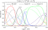 |
Fig. 9. Level-resolved carbon ionization equilibria with DR suppression for kappa distributions with κ = 2 (dashed), κ = 5 (dot-dashed), and for Maxwellian distribution (full lines) at constant pressure p = T × ne = 1016 K cm−3. Different colours correspond to different ions. |
4. Conclusions
In the present work, we have combined the effects of density and κ electron distributions in a CR model for carbon. This involved including collisional ionization, photoionization, and radiative and DR rates from ground and metastable levels, as well as suppression of DR with density. The interplay of these effects were tested at various densities, pressures, and kappa distributions, all in ionization equilibria. All of the effects are expected to be present in the Sun, and recent research has shown that they significantly affect the intensities of transition region lines (Dufresne & Del Zanna 2019; Dufresne et al. 2020, 2023).
In the present work, we find the following outcomes.
-
Level-resolved, direct ionization, and excitation-autoionization rates involving free electrons increase slightly with increasing electron densities. However, for most ions this effect is small compared to the changes with κ, except in the case of ionization from C III, which has a significant population of ions in metastable levels at transition region densities. At temperatures relevant for collisional ionization equilibrium, the ionization rates for kappa distributions are orders of magnitude higher than for Maxwellian distributions.
-
Level-resolved radiative and DR rates decrease with increasing density, while the peaks of the DR rates for low κ can be shifted to higher temperatures. Again, the changes seen in the recombination rates as electrons depart further from Maxwellian distributions are greater than the changes exhibited as electron densities increase. However, these changes to the recombination rates are much smaller than those seen for ionization.
-
The changes in level-resolved ionization and recombination rates with electron density lead to increases in relative ion abundances of C IV, as well as shifts of the lower charge-state ions to lower temperatures. The magnitude of these changes with density becomes progressively less important as κ decreases.
-
Photoionization is important only at low electron densities and higher values of κ. Its effect diminishes with decreasing κ due to large relative increase in the collisional ionization rates.
-
Density suppression of DR causes similar shifts in the ion balances as level-resolved ionization and recombination, that is, ion formation moves to lower temperature and peak ion abundances increase for the ions formed below 105 K. Suppression becomes weaker with decreasing κ, although at some temperatures and ions it can still be important.
-
The ionization equilibria were presented at various pressures typical of different regions on the Sun. The combined effect makes it clear that density effects are an important factor and improve on the coronal approximation, even where there are significant departures from Maxwellian energy distributions. However, they do not make as significant a change to the ion balances as when there are electron distributions with low κ values. This results from a complex interplay of how excitation, ionization, and recombination rates vary as electron distribution changes.
-
The overall changes caused by density are not as significant as the shifts to lower temperature and wider ranges of temperature formation that occur with increasing departures from a Maxwellian distribution.
Overall, the results mean that electron distributions with a very low κ have a much greater effect on the ionization equilibrium than adding the effects of electron density to the coronal approximation. The effects on line emission have not been tested here. That outcome depends very much on the temperature at which individual lines form and their relation to where the ion forms. This is likely to go on further to affect line ratios, especially for lines which form at different temperatures within the same ion.
As noted above, the outcome of this study does depend on the individual structure of each ion and the rates at which various atomic processes take place. This means that our conclusions here do not rule out the possibility that density effects may be important in ion formation of other elements in the presence of strongly non-Maxwellian electrons. Further studies will be required to assess this.
Acknowledgments
E.Dz. and J.D. acknowledge from the Czech Science Foundation, grant No. GACR 22-07155S, as well as institutional support RWO:67985815 from the Czech Academy of Sciences. G.D.Z. and R.P.D. acknowledge support from STFC (UK) via the consolidated grants to the atomic astrophysics group at DAMTP, University of Cambridge (ST/P000665/1 and ST/T000481/1). CHIANTI is a collaborative project involving George Mason University, the University of Michigan (USA), University of Cambridge (UK) and NASA Goddard Space Flight Center (USA).
References
- Arnaud, M., & Rothenflug, R. 1985, A&AS, 60, 425 [NASA ADS] [Google Scholar]
- Badnell, N. R. 2006, ApJS, 167, 334 [Google Scholar]
- Badnell, N. R., Pindzola, M. S., Dickson, W. J., et al. 1993, ApJ, 407, L91 [NASA ADS] [CrossRef] [Google Scholar]
- Badnell, N. R., O’Mullane, M. G., Summers, H. P., et al. 2003, A&A, 406, 1151 [NASA ADS] [CrossRef] [EDP Sciences] [Google Scholar]
- Bian, N. H., Emslie, A. G., Stackhouse, D. J., & Kontar, E. P. 2014, ApJ, 796, 142 [NASA ADS] [CrossRef] [Google Scholar]
- Bradshaw, S. J., Del Zanna, G., & Mason, H. E. 2004, A&A, 425, 287 [NASA ADS] [CrossRef] [EDP Sciences] [Google Scholar]
- Burgess, A., & Summers, H. P. 1969, ApJ, 157, 1007 [NASA ADS] [CrossRef] [Google Scholar]
- Curdt, W., Brekke, P., Feldman, U., et al. 2001, A&A, 375, 591 [NASA ADS] [CrossRef] [EDP Sciences] [Google Scholar]
- Del Zanna, G., & Mason, H. E. 2018, Liv. Rev. Sol. Phys., 15, 5 [Google Scholar]
- Del Zanna, G., Landini, M., & Mason, H. E. 2002, A&A, 385, 968 [NASA ADS] [CrossRef] [EDP Sciences] [Google Scholar]
- Del Zanna, G., Fernández-Menchero, L., & Badnell, N. R. 2015, A&A, 574, A99 [NASA ADS] [CrossRef] [EDP Sciences] [Google Scholar]
- Dere, K. P., Del Zanna, G., Young, P. R., & Landi, E. 2023, ApJS, 268, 52 [NASA ADS] [CrossRef] [Google Scholar]
- Doschek, G. A. 1984, ApJ, 279, 446 [NASA ADS] [CrossRef] [Google Scholar]
- Doschek, G. A., & Feldman, U. 1978, A&A, 69, 11 [NASA ADS] [Google Scholar]
- Doschek, G. A., & Mariska, J. T. 2001, ApJ, 560, 420 [NASA ADS] [CrossRef] [Google Scholar]
- Doschek, G. A., Dere, K. P., & Lund, P. A. 1991, ApJ, 381, 583 [NASA ADS] [CrossRef] [Google Scholar]
- Doschek, G. A., Warren, H. P., & Young, P. R. 2016, ApJ, 832, 77 [NASA ADS] [CrossRef] [Google Scholar]
- Doyle, J. G., & Raymond, J. C. 1984, Sol. Phys., 90, 97 [NASA ADS] [CrossRef] [Google Scholar]
- Doyle, J. G., Summers, H. P., & Bryans, P. 2005, A&A, 430, L29 [NASA ADS] [CrossRef] [EDP Sciences] [Google Scholar]
- Dudík, J., Del Zanna, G., Dzifčáková, E., Mason, H. E., & Golub, L. 2014, ApJ, 780, L12 [Google Scholar]
- Dudík, J., Polito, V., Dzifčáková, E., Del Zanna, G., & Testa, P. 2017, ApJ, 842, 19 [CrossRef] [Google Scholar]
- Dufresne, R. P., & Del Zanna, G. 2019, A&A, 626, A123 [NASA ADS] [CrossRef] [EDP Sciences] [Google Scholar]
- Dufresne, R. P., Del Zanna, G., & Badnell, N. R. 2020, MNRAS, 497, 1443 [NASA ADS] [CrossRef] [Google Scholar]
- Dufresne, R. P., Del Zanna, G., & Badnell, N. R. 2021a, MNRAS, 503, 1976 [NASA ADS] [CrossRef] [Google Scholar]
- Dufresne, R. P., Del Zanna, G., & Storey, P. J. 2021b, MNRAS, 505, 3968 [NASA ADS] [CrossRef] [Google Scholar]
- Dufresne, R. P., Del Zanna, G., & Mason, H. E. 2023, MNRAS, 521, 4696 [NASA ADS] [CrossRef] [Google Scholar]
- Dufresne, R. P., Del Zanna, G., Young, P. R., et al. 2024, ArXiv e-prints [arXiv:2403.16922] [Google Scholar]
- Dzifčáková, E. 1992, Sol. Phys., 140, 247 [CrossRef] [Google Scholar]
- Dzifčáková, E., & Dudík, J. 2013, ApJS, 206, 6 [CrossRef] [Google Scholar]
- Dzifčáková, E., & Kulinová, A. 2011, A&A, 531, A122 [NASA ADS] [CrossRef] [EDP Sciences] [Google Scholar]
- Dzifčáková, E., Dudík, J., Kotrč, P., Fárník, F., & Zemanová, A. 2015, ApJS, 217, 14 [CrossRef] [Google Scholar]
- Dzifčáková, E., Vocks, C., & Dudík, J. 2017, A&A, 603, A14 [NASA ADS] [CrossRef] [EDP Sciences] [Google Scholar]
- Dzifčáková, E., Dudík, J., Zemanová, A., Lörinčík, J., & Karlický, M. 2021, ApJS, 257, 62 [CrossRef] [Google Scholar]
- Dzifčáková, E., Dudík, J., Pavelková, M., Solarová, B., & Zemanová, A. 2023, ApJS, 269, 45 [CrossRef] [Google Scholar]
- Gontikakis, C., Winebarger, A. R., & Patsourakos, S. 2013, A&A, 550, A16 [NASA ADS] [CrossRef] [EDP Sciences] [Google Scholar]
- Hahn, M., & Savin, D. W. 2015, ApJ, 809, 178 [NASA ADS] [CrossRef] [Google Scholar]
- Hasegawa, A., Mima, K., & Duong-van, M. 1985, Phys. Rev. Lett., 54, 2608 [NASA ADS] [CrossRef] [Google Scholar]
- Hayes, M., & Shine, R. A. 1987, ApJ, 312, 943 [NASA ADS] [CrossRef] [Google Scholar]
- Jordan, C. 1969, MNRAS, 142, 501 [NASA ADS] [CrossRef] [Google Scholar]
- Judge, P. G., Woods, T. N., Brekke, P., & Rottman, G. J. 1995, ApJ, 455, L85 [NASA ADS] [Google Scholar]
- Laming, J. M., & Lepri, S. T. 2007, ApJ, 660, 1642 [NASA ADS] [CrossRef] [Google Scholar]
- Lazar, M., & Fichtner, H. 2021, Astrophys. Space Sci. Lib., 464, 299 [NASA ADS] [CrossRef] [Google Scholar]
- Livadiotis, G. 2017, Kappa Distributions: Theory and Applications in Plasmas, 1st edn. (Elsevier) [Google Scholar]
- Livadiotis, G., & McComas, D. J. 2009, J. Geophys. Res.: Space Phys., 114, A11105 [NASA ADS] [CrossRef] [Google Scholar]
- Ljepojevic, N. N., & MacNeice, P. 1988, Sol. Phys., 117, 123 [NASA ADS] [CrossRef] [Google Scholar]
- Mazzotta, P., Mazzitelli, G., Colafrancesco, S., & Vittorio, N. 1998, A&AS, 133, 403 [NASA ADS] [CrossRef] [EDP Sciences] [Google Scholar]
- Nikolić, D., Gorczyca, T. W., Korista, K. T., Ferland, G. J., & Badnell, N. R. 2013, ApJ, 768, 82 [CrossRef] [Google Scholar]
- Nikolić, D., Gorczyca, T. W., Korista, K. T., et al. 2018, ApJS, 237, 41 [CrossRef] [Google Scholar]
- Nussbaumer, H., & Storey, P. J. 1975, A&A, 44, 321 [NASA ADS] [Google Scholar]
- Olbert, S. 1968, Astrophys. Space Sci. Lib., 10, 641 [NASA ADS] [CrossRef] [Google Scholar]
- Olluri, K., Gudiksen, B. V., & Hansteen, V. H. 2013, ApJ, 767, 43 [NASA ADS] [CrossRef] [Google Scholar]
- Osterbrock, D. E. 1974, Astrophysics of Gaseous Nebulae (San Francisco: W.H. Freeman) [Google Scholar]
- Owocki, S. P., & Scudder, J. D. 1983, ApJ, 270, 758 [NASA ADS] [CrossRef] [Google Scholar]
- Peter, H., Tian, H., Curdt, W., et al. 2014, Science, 346, 1255726 [Google Scholar]
- Phillips, K. J. H., Feldman, U., & Landi, E. 2008, Ultraviolet and X-ray Spectroscopy of the Solar Atmosphere (Cambridge: Cambridge University Press) [CrossRef] [Google Scholar]
- Pinfield, D. J., Keenan, F. P., Mathioudakis, M., et al. 1999, ApJ, 527, 1000 [NASA ADS] [CrossRef] [Google Scholar]
- Polito, V., Del Zanna, G., Dudík, J., et al. 2016, A&A, 594, A64 [NASA ADS] [CrossRef] [EDP Sciences] [Google Scholar]
- Roussel-Dupré, R. 1980, Sol. Phys., 68, 243 [CrossRef] [Google Scholar]
- Shoub, E. C. 1983, ApJ, 266, 339 [NASA ADS] [CrossRef] [Google Scholar]
- Spadaro, D., Leto, P., & Antiochos, S. K. 1994, ApJ, 427, 453 [NASA ADS] [CrossRef] [Google Scholar]
- Summers, H. P. 1972, MNRAS, 158, 255 [NASA ADS] [CrossRef] [Google Scholar]
- Summers, H. P. 1974, MNRAS, 169, 663 [NASA ADS] [CrossRef] [Google Scholar]
- Summers, H. P., & Hooper, M. B. 1983, Plasma Phys., 25, 1311 [CrossRef] [Google Scholar]
- Vasyliunas, V. M. 1968a, J. Geophys. Res., 73, 2839 [NASA ADS] [CrossRef] [Google Scholar]
- Vasyliunas, V. M. 1968b, Astrophys. Space Sci. Lib., 10, 622 [NASA ADS] [CrossRef] [Google Scholar]
- Vocks, C., Dzifčáková, E., & Mann, G. 2016, A&A, 596, A41 [NASA ADS] [CrossRef] [EDP Sciences] [Google Scholar]
- Woods, T. N., Chamberlin, P. C., Harder, J. W., et al. 2009, Geophys. Res. Lett., 36, L01101 [NASA ADS] [CrossRef] [Google Scholar]
Appendix A: Comparison of methods for calculating ionization rates
Hahn & Savin (2015) developed a method for calculating rate coefficients for kappa distributions by using a weighted sum of Maxwellian rate coefficients. This is simpler than estimating the original cross-sections through inverting Maxwellian rate coefficients and then integrating over the desired distribution. This so-called Maxwellian decomposition method has been used in Sect. 3.3 for evaluation of the SFs of DR at higher densities, as also used in Dzifčáková et al. (2023). Because we had available ab initio, collisional ionization cross-sections for the present work, we decided to evaluate the performance and accuracy of the Maxwellian decomposition method.
We calculated the total ionization rate from the ground configuration of C III using direct integration of the cross-sections for various distributions, and compared them with the Hahn & Savin (2015) method. The comparison of the results is presented in Fig. A.1. It can be seen that the agreement is typically excellent. At relatively high temperatures, where the ionization rates are the strongest for all κ, the precision of the Hahn & Savin (2015) method is typically better than 1%. As the rates decrease with decreasing T, the precision does drop, but is typically still within about 10%. It is only at very low temperatures, where the ionization rates drop precipitously by orders of magnitude, that the precision worsens (see Fig. A.1). Nevertheless, when the Maxwellian decomposition method is used for DR suppression, as it is in the present work, such a situation does not occur because the SFs range between only 0 and 1. Thus, usage of the Hahn & Savin (2015) method does not lead to the introduction of additional uncertainties when using it for the DR suppression calculation.
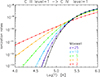 |
Fig. A.1. Collisional ionization rates together with excitation-autoionization rates for kappa distributions calculated from cross-sections (full lines) and using the Maxwellian decomposition method of Hahn & Savin (dot-dashed lines with diamonds). Different colours correspond to different distributions as indicated. |
Appendix B: Effect of DR suppression on the C ion abundances
To study the relative importance of the DR suppression on the Carbon ionization equilibria, we calculated these ionization equilibria for two cases. In the first one, only including level-resolved ionization and recombination rates are included (c.f., Sect. 3.1). In the second case, we include both the level-resolved ionization and recombination rates, as well as DR suppression.
Figure B.1 presents the ratio of these two cases. It is seen that for the Maxwellian distribution, the ion abundances can change by a factor of more than 1.5; this ratio reaches as much as 2.5 for C IV at some temperatures. However, the ratio diminishes with decreasing κ; it is in the range 0.5 – 1.4 for κ = 2 (see the top panel of Fig. B.1).
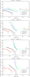 |
Fig. B.1. Ratios of level-resolved carbon ion fractions including DR suppression with respect to those without DR suppression, shown for different log(ne [cm−3]), as indicated, and for κ = 2, 5, 10, and Maxwellian distribution. Different colours correspond to different ions. |
All Tables
Excitation levels for which the individual ionization and recombination rates were calculated.
Maximum abundance of C IV as a function of ne and κ in ionization equilibrium including resolved ionization and recombination only.
Maximum abundance of C IV as a function of ne and κ in ionization equilibrium including resolved ionization and recombination, as well as density suppression of DR.
All Figures
|
Fig. 1. Comparison of the Maxwellian distribution with kappa distributions for κ = 10, 5, 3, and 2, at Temperature 5 × 10⁴ K. The different colours correspond to different distributions. |
| In the text | |
|
Fig. 2. Level populations in C II (left) and C III (right) plotted as a function of electron density log(ne [cm−3]). The temperature is indicated. The different colours correspond to different distributions. |
| In the text | |
|
Fig. 3. Level populations in C II (left) and C III (right) plotted as a function of temperature log(T [K]) at three different densities, log(ne [cm−3]) = 7, 9, and 11. The different colours correspond to different distributions. |
| In the text | |
|
Fig. 4. Dependence of the direct ionization (top panels) and excitation-autoionization rates (bottom panels) from C II → C III (left) and C III → C IV (right) at three different electron densities, log(ne [cm−3]) = 7, 9, and 11. The different colours correspond to different distributions, as indicated. The bottom right panel only shows the autoionization rate for κ = 2, 5, and Maxwellian for increased clarity (κ = 3 and 10 are omitted). |
| In the text | |
|
Fig. 5. Effect of metastable levels on the radiative (top), dielectronic (middle), and total recombination rates (bottom) for the recombination from C II → C I (left) and C III → C II (right), for three different electron densities, log(ne [cm−3]) = 7, 9, and 11, as indicated. The different colours correspond to different distributions. |
| In the text | |
|
Fig. 6. Carbon ionization equilibria including only ionization and recombination from/to excited levels, i.e., without DR suppression or photoionization, calculated for Log(ne/cm−3) = 7 (full lines), 9 (dashed lines), and 11 (dot-dashed lines), and for kappa distributions with κ = 2, 5, 10, and Maxwellian distribution. The different colours correspond to different ions. |
| In the text | |
|
Fig. 7. Level-resolved Carbon ionization equilibria including photoionization for quiet Sun without DR suppression shown for different log(ne [cm−3]) and κ = 2, 5, 10, and for Maxwellian distributions. The different colours correspond to different ions. |
| In the text | |
|
Fig. 8. Carbon ionization equilibria with ionization and recombination from density-dependent metastable states, DR suppression and photoionization for quiet Sun at constant pressures p = 1014(full lines), 1015 (dot-dashed), and 1016 K cm−3 (dashed) shown for κ = 2, 5, 10, and Maxwellian distributions. The thin dotted lines correspond to the ionization equilibrium using the coronal approximation, that is, without level-resolved ionization, recombination, DR suppression, and photoionization. |
| In the text | |
|
Fig. 9. Level-resolved carbon ionization equilibria with DR suppression for kappa distributions with κ = 2 (dashed), κ = 5 (dot-dashed), and for Maxwellian distribution (full lines) at constant pressure p = T × ne = 1016 K cm−3. Different colours correspond to different ions. |
| In the text | |
|
Fig. A.1. Collisional ionization rates together with excitation-autoionization rates for kappa distributions calculated from cross-sections (full lines) and using the Maxwellian decomposition method of Hahn & Savin (dot-dashed lines with diamonds). Different colours correspond to different distributions as indicated. |
| In the text | |
|
Fig. B.1. Ratios of level-resolved carbon ion fractions including DR suppression with respect to those without DR suppression, shown for different log(ne [cm−3]), as indicated, and for κ = 2, 5, 10, and Maxwellian distribution. Different colours correspond to different ions. |
| In the text | |
Current usage metrics show cumulative count of Article Views (full-text article views including HTML views, PDF and ePub downloads, according to the available data) and Abstracts Views on Vision4Press platform.
Data correspond to usage on the plateform after 2015. The current usage metrics is available 48-96 hours after online publication and is updated daily on week days.
Initial download of the metrics may take a while.