| Issue |
A&A
Volume 690, October 2024
|
|
|---|---|---|
| Article Number | A374 | |
| Number of page(s) | 20 | |
| Section | Stellar structure and evolution | |
| DOI | https://doi.org/10.1051/0004-6361/202450734 | |
| Published online | 22 October 2024 | |
Searching for new cataclysmic variables in the Chandra Source Catalog
1
Kazan Federal University, Kremlevskaya Str.18, 420008 Kazan, Russia
2
Department of Astronomy, California Institute of Technology, 1200 E. California Blvd, Pasadena, CA 91125, USA
3
Department of Astronomy, University of Washington, 3910 15th Avenue NE, Seattle, WA 98195, USA
4
Lawrence Berkeley National Laboratory, 1 Cyclotron Road, Berkeley, CA 94720, USA
5
Anton Pannekoek Institute for Astronomy, University of Amsterdam, 1090 GE Amsterdam, The Netherlands
6
IPAC, California Institute of Technology, 1200 E. California Blvd, Pasadena, CA 91125, USA
7
Division of Physics, Mathematics, and Astronomy, California Institute of Technology, Pasadena, CA 91125, USA
Received:
15
May
2024
Accepted:
30
July
2024
Abstract
Aims. Cataclysmic variables (CVs) are compact binary systems in which a white dwarf accretes matter from a Roche-lobe-filling companion star. For this study we searched for new CVs in the Milky Way in the Chandra Source Catalog v2.0, cross-matched with Gaia Data Release 3 (DR3).
Methods. We identified new CV candidates by combining X-ray and optical data in a color-color diagram called the X-ray main sequence. We used two different cuts in this diagram to compile pure and optically variable samples of CV candidates. We undertook optical spectroscopic follow-up observations with the Keck and Palomar Observatories to confirm the nature of these sources.
Results. We assembled a sample of 25 887 Galactic X-ray sources and found 14 new CV candidates. Seven objects show X-ray and/or optical variability. All sources show X-ray luminosity in the 1029 − 1032 erg s−1 range, and their X-ray spectra can be approximated by a power-law model with photon indices in the Γ ∼ 1 − 3 range or an optically thin thermal emission model in the kT ∼ 1 − 70 keV range. We spectroscopically confirmed four CVs, discovering two new polars, one low accretion rate polar and a WZ Sge-like low accretion rate CV. X-ray and optical properties of the other nine objects suggest that they are also CVs (likely magnetic or dwarf novae), and one other object could be an eclipsing binary, but revealing their true nature requires further observations.
Conclusions. These results show that a joint X-ray and optical analysis can be a powerful tool for finding new CVs in large X-ray and optical catalogs. X-ray observations such as those by Chandra are particularly efficient at discovering magnetic and low accretion rate CVs, which could be missed by purely optical surveys.
Key words: binaries: close / binaries: eclipsing / stars: dwarf novae / novae / cataclysmic variables / X-rays: binaries
Corresponding author; This email address is being protected from spambots. You need JavaScript enabled to view it.
© The Authors 2024
 Open Access article, published by EDP Sciences, under the terms of the Creative Commons Attribution License (https://creativecommons.org/licenses/by/4.0), which permits unrestricted use, distribution, and reproduction in any medium, provided the original work is properly cited.
This article is published in open access under the Subscribe to Open model. This email address is being protected from spambots. You need JavaScript enabled to view it. to support open access publication.
1. Introduction
Cataclysmic variables (CVs) are compact semidetached binaries in which a white dwarf (WD) accretes matter from a Roche-lobe-filling companion star (Warner 2003). CVs have orbital periods typically spanning 66 min–10 h, except for ultra-compact AM Canum Venaticorum (AM CVn) stars, which have ≲1 h periods (Ramsay et al. 2018). In magnetic CVs, the magnetic field of the WD (B ≳ 1 MG) significantly influences the accretion onto the surface of the WD. Magnetic CVs are split into intermediate polars (IPs), which have truncated disks, and polars, where the strong field (B ∼ 10 − 250 MG) prevents disk formation. Studies of CVs augment our understanding of various astrophysical phenomena, including their role as potential progenitors for Type Ia supernovae (Maoz et al. 2014). They also present optimal nonrelativistic laboratories to study accretion processes (Hameury 2020). Furthermore, due to their short orbital periods, some CVs and many ultra-compact AM CVn systems are classified as prospective verification binaries for future planned space-based gravitational wave observatories such as LISA (Kupfer et al. 2024).
From the theoretical standpoint, CVs are predicted to form as a result of common envelope evolution (CEE; Paczynski 1976; Ivanova et al. 2013) that first brings the stars closer together. Angular momentum loss (AML) is the key factor in the long-timescale evolution of CVs. As AML occurs, the separation between the stars decreases, leading to a reduction in the orbital period. The evolutionary model considers two mechanisms for AML: magnetic wind braking (Rappaport et al. 1983; Spruit & Ritter 1983) and gravitational-wave radiation (Paczyński 1967; Faulkner 1971). Although the model initially aligned well with the observational data of that era, subsequent findings revealed numerous discrepancies between theory and observations (e.g., Patterson 1998; Gänsicke et al. 2009; Pretorius & Knigge 2012; El-Badry et al. 2022). Consequently, empirical revisions were proposed to rectify these inconsistencies (e.g., Knigge et al. 2011; Schreiber et al. 2016, 2021).
Cataclysmic variables exhibit a broad range of observational features, and therefore detailed multiwavelength studies are necessary to draw accurate conclusions about their nature and population. X-ray emission analysis is a powerful tool for searching for and studying CVs. The first X-ray observations of CVs took place with HEAO-1 (Cordova et al. 1981) and Einstein (Cordova & Mason 1984). Early X-ray surveys led to the discovery of a unique previously unidentified population of magnetic CVs (e.g., Haberl & Motch 1995). The all-sky X-ray survey conducted by the eROSITA telescope aboard the Spektrum-Roentgen-Gamma (SRG) mission (Sunyaev et al. 2021; Predehl et al. 2021) is proving to be groundbreaking; it is cataloging millions of sources (Merloni et al. 2024) and has already been successful in discovering a collection of new and rare CVs due to its ability to reach much fainter fluxes (e.g., Schwope et al. 2022a,b; Rodriguez et al. 2023a; Galiullin et al. 2024).
Although it is not an all-sky X-ray survey, the Chandra observatory provides unique subarcsecond on-axis resolution that is comparable with optical surveys (Weisskopf et al. 2000, 2002). The Chandra Source Catalog v2.0 (hereafter, CSC2) provides the uniformly calibrated science-ready data products compiled from the archival Chandra data (Evans et al. 2010). Such data collection enables the study of the properties of X-ray sources with spectral and timing analyses and the classification of new objects in the catalog. In addition to new X-ray surveys and catalogs, all-sky optical photometric surveys provide a wealth of new data. The Zwicky Transient Facility (ZTF) is the deepest northern sky time-domain photometric survey, conducted at Palomar Observatory on the Samuel Oschin 48-inch telescope. The 47 deg2 field of view camera images the sky roughly every two days down to ∼20.5 mag in g, r, and i filters (Bellm et al. 2019; Graham et al. 2019; Dekany et al. 2020; Masci et al. 2019).
For this paper our aim was to search for and study new CVs in the CSC2, cross-matched with the third Gaia Data Release (hereafter, Gaia DR3). In Sect. 2 we describe the construction steps of a sample of Galactic X-ray sources based on the CSC2–Gaia DR3 catalog. In Sect. 3 we describe the selection of new CV candidates in the CSC2–Gaia DR3 catalog using two different cuts in the X-ray and optical color-color diagram, known as the X-ray main sequence. We compiled pure and optically variable samples of CV candidates. In Sect. 4 we present the follow-up observations conducted with the 5 m Hale Telescope at Palomar Observatory and the 10 m Keck I Telescope on Mauna Kea. We also present detailed X-ray timing and spectroscopic analyses. In Sect. 5 we present the sample of 14 CV candidates found in the CSC2–Gaia DR3 catalog. We separately discuss the nature of four spectroscopically confirmed CVs and four variable CV candidates. Our results are summarized in Sect. 6.
2. Sample of Galactic X-ray sources
We began by constructing a sample of Galactic X-ray sources from the publicly available CSC2 (Evans et al. 2010). We cross-matched CSC2 with the Gaia DR3 catalog (Gaia Collaboration 2023), keeping only objects with significant parallaxes and proper motions. We identified the known sources in our sample by cross-matching with the Simbad database and other publicly available CV catalogs. All sample creation steps are presented in detail below.
2.1. Chandra source catalog
As a first step, we used the master source table from the CSC2 with a total of about ∼317 000 unique source detections. We set the following criteria1 to select the point-like X-ray sources with measured parameters:
-
extent_flag = False; only point-like sources.
-
conf_flag = False; source regions do NOT overlap.
-
pileup_flag = False; ACIS pile-up fraction does NOT exceed ∼10% in all observations.
-
sat_src_flag = False; the source is NOT saturated in all observations.
-
streak_src_flag = False; the source is NOT located on an ACIS readout streak in all observations.
-
dither_warning_flag = False; highest statistically significant peak in the power spectrum of the source region count rate does NOT occur at the dither frequency of the observation.
-
man_add_flag = False and man_inc_flag=False; the source was NOT manually added nor included in the catalog via human review.
-
man_match_flag = False; source detections were NOT manually matched between overlapping stacked observations via human review.
-
man_pos_flag = False; best-fit source position was NOT manually modified via human review.
-
man_reg_flag = False; source region parameters were NOT manually modified via human review.
Using these criteria, we selected 271 438 unique objects from CSC2.
2.2. Cross-match with Gaia
For the next step we cross-matched 271 438 objects with the Gaia DR3 catalog (Gaia Collaboration 2023) to select only Galactic sources. As a search radius for each object, we used the individual X-ray positional error (with a search radius equal to err_ellipse_r0, the semimajor axis of the 95% confidence ellipse). We only kept sources meeting the following criteria:
-
RUWE < 1.4 (as recommended in Gaia Collaboration 2023); good fit to the astrometric observations.
-
Only ONE Gaia object must be within the search radius.
-
Parallax and proper motion are measured with a signal-to-noise ratio S/N ≥ 3.
These selection steps reduced the number of sources to 26 079. To remove any potential high proper motion stars, we applied an additional filtering criterion:
-
pm × Δt ≤ err_ellipse_r0; The angular motion of the Gaia object (caused by a proper motion, pm) during the time interval Δt does not exceed the search radius (err_ellipse_r0). The time interval Δt is an epoch difference between Gaia DR3 (Epoch 2016) and CSC2 (Epoch 2000) catalogs.
This filter finally resulted in 25 887 objects in the CSC2–Gaia DR3 catalog.
2.3. Identification of known sources
To identify known sources in the CSC2–Gaia DR3 catalog, we cross-matched our objects with the Simbad database (Wenger et al. 2000) using Gaia coordinates and a 3″ search radius. We grouped our objects, based on the Simbad hierarchical structure2, into seven general categories: STARS (single and binaries), ACCRETING BINARIES (X-ray binaries, CVs, Novas, and Symbiotic Stars), GALAXY, ISM, PROPERTIES, BLENDS (not well-defined objects), and UNKNOWN (object is not presented in Simbad database). In Appendix A we present a detailed description of our general object types compiled from the Simbad hierarchical structure. We found Simbad classifications for 12 1813 of the 25 887 objects; 32 of the 12 181 objects were known CVs or CV candidates.
To check that we did not miss any known CVs, we independently cross-matched our 25 887 objects with the following catalogs using a 2″ search radius: (i) the Ritter and Kolb catalog (Ritter & Kolb 2003, Final version; December 31, 2015); (ii) the Cataclysmic Variables Catalog (2006 edition; Downes et al. 2001; iii) the Open Cataclysmic Variable Catalog (Jackim et al. 2020, only confirmed CVs are kept in the list). We combined the information from the Simbad database and these three CV catalogs to make the final list of known CVs. Out of 25 887 sources, we finally compiled a sample of 40 known CVs. This sample of 40 consists of the CVs from Simbad plus those from the three catalogs mentioned above.
It should be noted that 52 objects (out of 25 887) were classified as GALAXY. These objects are primarily quasars and galaxies hosting active galactic nuclei that show significant parallax and proper motion. The high proper motions and parallaxes of these extragalactic objects could be due to variability-induced motion (e.g., Souchay et al. 2022; Makarov & Secrest 2022; Khamitov et al. 2023). A detailed investigation of these objects is beyond the scope of this paper.
3. CV selection with the X-ray main sequence
We combined X-ray and optical data to search for new CV candidates in the CSC2–Gaia DR3 catalog. We used the X-ray main sequence, a phase space of X-ray-to-optical flux ratio (FX/Fopt) and a Gaia optical BP–RP color (Rodriguez 2024), to select CV candidates and create a pure sample of these objects. The empirical cut in the X-ray main sequence is given by the functional form
 (1)
(1)
where A = −3.5 and B = 1 are linear parameters from Rodriguez (2024). We computed the FX/Fopt ratio based on X-ray and Gaia optical fluxes. The X-ray fluxes were calculated in the 0.5–7 keV energy band from CSC2. The aperture-corrected (90% enclosed counts fraction) energy flux is calculated using the power-law model with a photon-index of Γ = 2 and the individual Galactic hydrogen column density NH(Gal) in the direction of the source. Gaia G band magnitudes were converted to optical fluxes using the AB magnitude system and a central wavelength of 6000 Å. Out of 25 887 sources in the CSC2–Gaia DR3 catalog, we selected only sources with measured X-ray fluxes and optical magnitudes:
-
flux_powlaw_aper90_b/error ≥ 2; Source X-ray flux in the 0.5–7 keV energy band is measured with a signal-to-noise ratio higher than S/N ≥ 2.
-
Gaia G band, BP and RP magnitudes are measured having a signal-to-noise ratio higher than S/N ≥ 2.
These selection steps finally resulted in 19 665 sources (with 36 known CVs).
3.1. First selection: Pure sample of CV candidates
To compile a pure sample of CV candidates and avoid contamination from stellar objects, we searched for optimal values for linear parameters A and B in Eq. (1). We created two samples of known sources classified based on the Simbad hierarchical structure, one consisting of CVs (36 sources) and the other of stellar objects (STARS, 4781 sources). For the STARS sample, we included only objects with subtypes classified as YSOs, Binaries, Massive Stars, Main Sequence Stars, or Evolved Stars (see Table A.1). The left panel of Fig. 1 shows an FX/Fopt and Gaia BP–RP color diagram for known CVs (red squares) and STARS (blue dots). It is evident that known CVs are primarily located in the upper left corner of the diagram and could be visually separated from STARS. We computed the purity and completeness using a sample of these known CVs and STARS (see Appendix A for more details). Based on our completeness–purity analysis we selected A = −1.5, and B = 0.7, which gives the highest purity (≈100%) and ≈52% completeness.
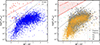 |
Fig. 1. X-ray-to-optical flux ratio vs Gaia (BP–RP) optical color (X-ray main sequence; Rodriguez 2024) for objects in the CSC2–Gaia DR3 catalog. Left panel: Known CVs (red) and stellar objects (STARS, blue) in the CSC2–Gaia DR3 catalog. The dashed black line shows an empirical cut from Rodriguez (2024). The solid red line shows a cut to select a pure sample of CV candidates. Right panel: Objects in the CSC2–Gaia DR3 catalog with the Simbad classifications (which may be imprecise). The colored symbols correspond to the different object types based on the Simbad hierarchical structure (see Table A.1). Objects above the solid red line and variable objects above the dashed black line are classified as new CV candidates (see Tables 1 and B.1). For more details, see Sect. 3. |
New CVs and their candidates found in the CSC2–Gaia DR3 catalog.
We only searched for new CV candidates among objects without precise classifications from the Simbad database. Out of 19 665 objects, we selected 13 956 sources classified as one of the following object types: (i) UNKNOWN (9868 sources); (ii) PROPERTIES (355 sources); (iii) STARS, subtype Star (3720 sources); (iv) STARS, subtype WD (10 sources); (v) STARS, subtype BD (3 sources). The right panel of Fig. 1 shows the FX/Fopt and Gaia BP–RP color diagram for these objects. We found 11 new CV candidates (out of 13 956 objects) with our selection based on our optimal values for A = −1.5 and B = 0.7 (see objects above the solid red line in the right panel of Fig. 1).
We note that we independently found three objects (recently confirmed as CVs) as CV candidates using the FX/Fopt and Gaia (BP–RP) color diagram. During the writing of this manuscript, we learned that these systems had been previously discovered. However, these objects have only been mentioned in one or two papers, so we included them in our analysis and discuss them individually in Appendix B.
3.2. Second selection: Optically variable sample of CV candidates with ZTF photometry
Many CVs appear as periodic sources in optical light curves. Furthermore, accretion can lead to outbursts, which can also be observed in their optical light curves, particularly in nonmagnetic CVs. Therefore, even after compiling a sample of 11 CV candidates based purely on an FX/Fopt and a Gaia BP–RP color diagram, we also searched for possible variability in a larger sample of sources. We used the empirical cut on the FX/Fopt and Gaia BP–RP color diagram from (Rodriguez 2024, A = −3.5 and B = 1) and searched for possible variability in 375 sources (see objects above the dashed black line in the right panel of Fig. 1).
We searched for periodic and outbursting-type variability in sources based on ZTF optical photometry for both g and r light curves, considering only data with a signal-to-noise ratio greater than 5, S/N ≥ 5. We retrieved ZTF light curves for our objects and used the barycentric corrected modified Julian date (MJD) in our analysis. Light curves have a photometric precision of ∼0.015 mag at the bright limit of 14 mag, decreasing to a precision of ∼0.1 mag at the faint limit of 20.5 mag. We searched for periodic variability using the Lomb–Scargle periodogram, as implemented in the gatspy tool to search for periods ranging from five minutes to ten days. Once the period search was performed, we excluded all sources with orbital periods that are multiples or fractions of the sidereal day. To first order, the periods are reported up to a precision of 30 s, which is determined by the exposure time. To calculate the significance of a period, we first computed the median absolute deviation (MAD) of the periodogram. Then, we took the periodogram value at the highest peak and divided it by the MAD. This ratio served as our significance metric. We plotted the distribution of significance metrics and kept only those sources in the upper 80th percentile of the distribution. To search for outbursting sources, we looked for ZTF light curves with more than five outburst points Δmag ≥ 1, with each point more than three standard deviations from the median.
In total, we had 178 (out of 375) sources with ZTF photometry. Using our selection criteria described above, we found five periodic sources (see Figs. 2, 3, 4, and 5). With ZTF photometry, only one outbursting source (2CXO J024131.0+593630) was identified, which we discuss in Appendix B. Based on the analysis of optical ZTF light curves, we extended our final sample of CV candidates to include a total of 14 candidates4.
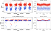 |
Fig. 2. ZTF long-term (left) and phase-folded (right) light curves for 2CXO J173118.6+224248 (top panel) and 2CXO J185603.2+021259 (bottom panel) in g (blue) and r (red) filters. |
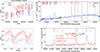 |
Fig. 3. ZTF long-term (top left) and phase-folded (bottom left) light curves in g and r filters and the DBSP optical spectrum of 2CXO J044048.3+292434 (right). The gray lines represent the Keck Telluric Line List. The optical spectrum (top right) shows the hydrogen Balmer and helium emission lines and high-excitation He II 4686 Å emission line, giving a high line ratio He II/Hβ ≈ 0.64 (see Table 3). Optical and X-ray properties indicate that the object is a polar. Bottom right panel: Since two spectra taken 1.4 h apart do not show a significant radial velocity shift (a ≈ 1000 km/s shift would be expected if this were half of the orbital period and the system were viewed edge-on), the 1.3 h period is preferable. However, time-resolved spectroscopy for 2.6 h would be the only way to confirm the orbital period of this system, leading us to currently label the orbital period as either 1.3 or 2.6 h (see Sect. 5.1.1 for more details). |
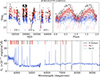 |
Fig. 4. ZTF long-term (top left) and phase-folded (top right) light curves in g, r, and i filters and the DBSP optical spectrum of 2CXO J123727.5+655211 (bottom). The gray lines represent the Keck Telluric Line List. The optical spectrum shows hydrogen, helium, and high-excitation He II 4686 Å emission lines, giving a line ratio of He II/Hβ ≈ 0.37 (see Table 3). Together with optical light curves, this indicates that the object is a polar (see Sect. 5.1.3 for more details). |
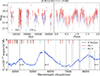 |
Fig. 5. ZTF long-term (top left) and phase-folded (top right) light curves in g and r filters and the DBSP optical spectrum of 2CXO J182117.2–131405 (bottom). The gray lines represent the Keck Telluric Line List. The optical spectrum is dominated by broad humps that correspond to cyclotron harmonics, and no significant Hβ and He II 4686 Å emission lines are detected. A combination of the cyclotron wavelengths seen in the spectrum and the large beaming amplitude constrains the magnetic field to B ≈ 54 − 63 MG. Optical and X-ray properties suggest that the object is a low accretion rate polar (see Sect. 5.1.4 for more details). |
Out of 14 sources, two objects were marked as variables with a Gaia flag (phot_variable_flag=VARIABLE). These objects show outbursting-type variability. Figure 6 shows optical light curves based on Gaia photometry (S/N ≥ 3). Table 1 (Col. 9) summarizes the variability properties of the sources in the final sample. We note that the number of spurious matches in our final sample is effectively zero due to the ∼1–2′ localization of X-ray sources made possible by Chandra. Furthermore, our candidates that show optical variability are even less likely to be false matches since optical variable sources, particularly accreting compact objects, are typically associated with X-ray emission (e.g., see Fig. 2 in Rodriguez 2024).
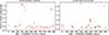 |
Fig. 6. Gaia long-term light curves in G band for two sources in our sample. Panels: 2CXO J063805.1–801854 (left) and 2CXO J165219.0–441401 (right). |
4. Data and analysis
4.1. Optical spectra
We performed optical spectroscopic follow-up observations for four sources in our sample, focusing on those located in the northern hemisphere that were accessible to our telescopes and exhibited strong optical variability and/or a high FX/Fopt ratio. We used both the Double Spectrograph (DBSP; Oke & Gunn 1982) on the 5 m Hale Telescope at Palomar Observatory and the Low-Resolution Imaging Spectrometer (LRIS; Oke et al. 1995) at the 10 m Keck I Telescope on Mauna Kea. During all DBSP observations, we used the 600/4000 grism on the blue side and the 316/7500 grating on the red side. A 1.5″ slit was used, and the seeing on all occasions was 1.5–2.0″. All P200/DBSP data were reduced with DBSP-DRP5, a Python-based pipeline built upon the existing PypeIt package (Prochaska et al. 2020) and optimized for reducing spectral data. During all LRIS observations, we used the 600/4000 grism on the blue side and the 600/7500 grating on the red side. We used a 1.0″ slit, and the seeing on all occasions was around 0.7″. LRIS data were reduced with lpipe, an IDL-based pipeline optimized for LRIS long-slit spectroscopy (Perley 2019). All data were flat-fielded and sky-subtracted using standard techniques, wavelength-calibrated with internal arc lamps, and flux-calibrated using a standard star. Table 2 shows all data acquired for the four CV candidates. Single spectra were taken at a time for each object (no coadds), with typical exposure times of 600 seconds for Keck I/LRIS and 900 seconds for P200/DBSP.
Data acquired for CV candidates.
Figure 7 shows Chandra X-ray images and optical images from Pan-STARRS (Chambers et al. 2016) of the same sky region for four spectroscopically confirmed CVs in our sample. Figures 3–5 and 8 show the optical spectra of these sources. We identified prominent emission lines and computed their equivalent widths (EWs) by fitting Gaussian profiles to them. Table 3 shows the EWs of selected lines and the He II(4686)/Hβ ratio6.
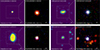 |
Fig. 7. X-ray and optical images for four new spectroscopically confirmed CVs from CSC2–Gaia DR3 catalog. Left: False-color Chandra X-ray images in the 0.5–7 keV energy band. The images were smoothed using a Gaussian kernel with different widths equal to 1 − 3 times the PSF radius, depending on the source counts. Right: Composite optical images based on Pan-STARRS i, r, and g filter data. The white boxes show the field of view of the optical images on the right. Circles: a PSF radius equal to the 90% of encircled counts fraction (solid white line), and a radius equal to the semimajor axis of the error ellipse (95% localization error) centered on the source X-ray position (dashed magenta line). |
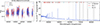 |
Fig. 8. ZTF long-term light curves in g and r filters (left) and DBSP optical spectrum of 2CXO J044147.9–015145 (right). The gray lines represent the Keck Telluric Line List. The optical spectrum shows WD Balmer absorption lines with no sign of the donor signature, weakly double-peaked hydrogen and helium emission lines, and no detectable He II 4686 Å emission line, giving a 3σ upper limit for the line ratio He II/Hβ < 0.05 (see Table 3). Optical and X-ray properties suggest that the object is a CV (WZ Sge type; see Sect. 5.1.2 for more details). |
Equivalent widths (−EW(Å)) of selected lines of four spectroscopically confirmed CVs.
We conducted an extensive cross-match analysis between our 14 objects and publicly available optical data from the Sloan Digital Sky Survey (SDSS) and the Dark Energy Spectroscopic Instrument (DESI) collaboration (DESI Collaboration 2016). With 2″ search radius, we found no matches between the SDSS/APOGEE catalogs (APOGEE DR17 StarHorse VAC, Queiroz et al. 2020; APOGEE DR17 astroNN VAC, Mackereth et al. 2019; APOGEE DR17 DistMass VAC, Stone-Martinez et al. 2024; APOGEE Net VAC Sprague et al. 2022; MaStar Stellar Parameters VAC, Lazarz et al. 2022); and our CV sample. We cross-matched our objects with the early data release (EDR) of DESI collaboration (DESI Collaboration 2024), which contains spectra of more than one million objects (DESI Collaboration 2024). We found no identification of our objects with this catalog.
4.2. X-ray spectra and luminosities
For each of the 14 sources in our sample, we queried the archival Chandra data using the observation identifier (obsid) from source observation summary results in the CSCview application7. For some objects we additionally searched for new Chandra observations within a 10′ search radius using the Chaser8 webtool and included them in our analysis. The Chandra archival observations were processed by following standard Chandra Interactive Analysis of Observations (CIAO; Fruscione et al. 2006) threads9 (CIAO version 4.16.0 and CALDB version 4.11.0). The chandra_repro tool was used to perform the initial calibration, to reprocess the data, and to create a level 2 event file. To extract the source and background spectra, we used the specextract tool in CIAO. A point-source aperture correction was applied for each source spectra by setting the parameter correctpsf = yes. We computed the radii of the Chandra point spread function (PSF) from the PSF map, which was constructed with mkpsfmap tool for 90% of encircled counts fraction (ECF) and the 2.3 keV energy (parameters ecf = 0.9 and energy = 2.3 respectively). Source and background regions were centered at source positions from CSC2. A circle with radius equal to the Chandra PSF radius was used for the source regions, and annuli with the inner and outer radii equal to two and four times the Chandra PSF radius were used for background regions.
We performed the spectral fit using the XSPEC v12.13 package (Arnaud 1996) in the 0.5–7 keV energy band. We binned the X-ray spectra to have at least three counts per bin, and used C-statistics (Cash 1979) to get best-fit results. We used the error command in XSPEC to compute 1σ confidence intervals for the parameters. For some sources in our sample, we estimated only the 1σ lower limit (or upper limit) of the parameters. Each spectrum was approximated using two spectral models: the power-law model (powerlaw in XSPEC) and the optically thin thermal plasma emission model (mekal in XSPEC). To take into account interstellar absorption, we used the Tuebingen-Boulder ISM absorption model (tbabs in XSPEC) and the solar elemental abundances from Wilms et al. (2000).
All sources in our sample are located at different distances, leading to various Galactic hydrogen column densities. We computed the distances of the sources from Gaia parallaxes, and their errors were calculated using the standard error propagation. Using the source distances, we adopted the E(B − V) values from the Bayestar dust map (Green et al. 2019). If data from the Bayestar dust map were not available, we utilized the Galactic plane reddening map (Chen et al. 2019). We computed the hydrogen column density by assuming Cardelli’s extinction law (RV ≈ 3.1) and the relation NH(map) ≈ RV × E(B − V)×2.21 × 1021 cm−2 (Cardelli et al. 1989; Güver & Özel 2009). For sources with more than 100 counts in their X-ray spectra, we computed the hydrogen column density (NH(fit)) and metal abundance directly from the fit. We found no significant deviation between the best-fit results of NH(fit) and NH(map) computed from the Bayestar dust map. For other sources, we approximated their spectra with a fixed NH(map) and assuming solar metallicity. In the cases when NH(map) was not available at the specified distance of the source or when the distance fell outside the interval classified as reliable, we fixed the hydrogen column density to the Galactic value (HI4PI Collaboration 2016).
The best-fit results obtained from approximating the X-ray spectra with powerlaw and mekal models are presented in Appendix C (see Table C.1 and Fig. C.1). For sources with more than one Chandra observation, we analyzed the X-ray spectra for each observation separately. However, we found no significant parameter variations between these separate observations, and subsequently performed a joint fit of the spectra in XSPEC by combining the parameters across multiple observations. We computed absorption corrected fluxes in the 0.5–7 keV energy band for the power-law model using the cflux command and converted them to luminosities. The approximate errors of the unabsorbed X-ray luminosities were computed from the uncertainties in the distances and fluxes using standard error propagation. Table 1 (Cols. 10 and 11) shows the distances and unabsorbed X-ray luminosities in the 0.5–7 keV energy band.
4.3. X-ray variability and timing analysis
We searched our sample of 14 CV candidates for X-ray variable sources using the CSC2 variability indices in the 0.5–7 keV energy band: var_intra_index_b ≥ 8 (variability within a single observation) and/or var_inter_index_b ≥ 8 (variability across multiple observations). We found only one source matching these criteria (2CXO J063805.1–801854). We also checked the significance of the difference between the maximum and minimum fluxes between observations using the ratio R = (Fmax − Fmin)/(σFmax2 + σFmin2)1/2 and found only one source having R ≥ 3 (2CXO J123727.5+655211).
Out of the 14 CV candidates in our sample, we performed an X-ray timing analysis for three sources with more than 300 source counts in their spectra (see Table 4). If sources had more than one archival Chandra observation, we used the observation with the longest exposure time for the timing analysis. We extracted the background-subtracted X-ray light curves with the dmextract tool in CIAO, using the same source and background regions as those used for the X-ray spectral analysis. Barycentric corrections were applied for the event files by using axbary tool in CIAO. We used the XRONOS subpackage in FTOOLS10 for timing analysis NASA High Energy Astrophysics Science Archive Research Center (HEASARC) (2014). First, we calculated the power spectrum density using a fast Fourier transform (powspec command in the XRONOS package) to search for periodic signal. The epoch-folding (EF) technique was then applied to constrain the period of the sources (Larsson 1996) using the efsearch command in the XRONOS package. We estimated the best-fit period from the EF method by fitting a Gaussian function to the χ2 versus period diagram. The period error was estimated using a bootstrap technique similar to that described in Boldin et al. (2013). To determine the significance of the detected period, we generated 1000 random Poisson nonperiodic light curves with mean source count rates, and applied the powspec and efsearch tools to these randomly generated light curves. We computed the maximum value of the power spectrum density and the χ2 (as defined in the EF method) for each generated light curve. A 3σ upper confidence level was calculated for the distributions of power spectrum densities and χ2 values. A strong signal was considered present in the observed X-ray light curves if the results from the powspec and efsearch tools exceeded the 3σ confidence level determined from the simulations. We then used the efold tool to construct X-ray light curves folded with the best-fit periods.
List of CV candidates used to search for X-ray periodic signals.
We found strong periodic X-ray signals only in one source out of three (see Table 4). Figure 8 shows the X-ray pulse profile normalized by the mean count rate of that source. The pulse fraction (PF) was computed using maximum and minimum count rates, where PF = (Fmax − Fmin)/(Fmax + Fmin). We discuss the nature of the X-ray periodic source in Sect. 5.2.
4.4. Hertzsprung-Russell and X-ray luminosity–orbital period diagrams
To compute extinction-corrected absolute G band magnitudes for CV candidates, we directly adopted the interstellar extinction AG (at 6000 Å) from Bayestar or the Galactic plane reddening maps when available. Otherwise, we converted the hydrogen column densities presented in Table C.1 for the mekal model (see Sect. 4.2) to interstellar extinction AG using the Cardelli et al. (1989) extinction function. Figure 9 shows the location of the CV candidates on the Hertzsprung-Russell (HR) diagram along with Gaia objects within 100 pc that have significantly measured parallaxes (parallax_over_error > 3).
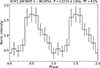 |
Fig. 9. Chandra X-ray pulse profile for 2CXO J063805–801854 normalized by mean count rate 0.01 cnt s−1. |
We constructed an X-ray luminosity–orbital period diagram for six objects in our sample with periods computed from the optical and X-ray data (see Fig. 10). To compare our objects with other known CVs, we cross-matched the CV catalog of Ritter and Kolb (final edition, frozen on 31 December 2015; Ritter & Kolb 2003) with the second ROSAT all-sky survey (2RXS) catalog (Boller et al. 2016), keeping only sources with a single match within 20″. We then cross-matched with Gaia DR3 (Gaia Collaboration 2023), keeping only sources with significant parallaxes and proper motions (5σ), which yielded 259 sources. Next we used the WebPimms11 tool to convert the ROSAT source count rates (0.1–2.4 keV) to unabsorbed X-ray luminosities in the 0.5–7 keV energy band, assuming a power-law model with a photon index of 1.7 and hydrogen column density of 3 × 1020 cm−2. To show different CV types in Fig. 10, we used the classification scheme of the Ritter and Kolb catalog, which categorizes them as polar (AM) or intermediate polar (DQ), or otherwise as nonmagnetic. In Fig. 10 we show different period minimum values for CVs from Gänsicke et al. (2009) (≈82 min) and Knigge (2006) (≈76 min) as well as CV orbital period gap values from Schreiber et al. (2024) (≈2.5 − 3.2 h) and Knigge (2006) (≈2.2 − 3.2 h).
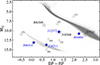 |
Fig. 10. Extinction-corrected Hertzsprung-Russell (HR) diagram. All Gaia sources within 100 pc with significantly measured parallaxes (parallax_over_error > 3) are shown in gray (Gaia Collaboration 2023). The star markers represent new spectroscopically confirmed CVs (blue) and variable CV candidates (white) from Table 1. The white circles indicate CV candidates selected by a FX/Fopt ratio and Gaia (BP–RP) color: (1) J165219.0–441401; (2) J173332.5–181735; (3) J094607.7–311550; (4) J155926.5–754311; (5) J190823.2+343328; (6) J173555.3–292530. |
5. Results and discussion
Table 1 shows the parameters of the 14 CV candidates found in the CSC2–Gaia DR3 catalog using the FX/Fopt and the Gaia BP–RP color diagram and the period search with ZTF optical photometry (see Sect. 3). Figure 9 shows that most of our CV candidates are located between the main sequence and the WD regions, which is consistent with the distribution of known CVs in the Gaia HR diagram (e.g., Abril et al. 2020). The X-ray luminosities of all our objects vary in the ≈1029 − 1032 erg s−1 range, which matches the range of X-ray luminosities of some known CVs (see Fig. 10). The X-ray spectra of our CV candidates can be approximated by a power-law model with photon indices in the Γ ≈ 1 − 3 range (or kT ∼ 1 − 70 keV for the optically thin thermal emission model). Such X-ray spectra are seen in some magnetic and nonmagnetic CVs (e.g., Galiullin & Gilfanov 2021; Schwope et al. 2022a,b; Rodriguez et al. 2023a; Galiullin et al. 2024).
Our variability search indicates that seven sources out of these 14 CV candidates are variable in nature. The X-ray luminosity–orbital period diagram shows that most of our variable sources have X-ray luminosities and periods typically seen for magnetic and nonmagnetic CVs (see Fig. 10). Only two sources (2CXO J182117.2–131405 and 2CXO J185603.2+021259) are located in a distinct region of the phase space compared to the main sample of CVs, and exhibit low X-ray luminosity. These two objects might be a low accretion rate CV and an eclipsing binary12. We spectroscopically confirm four objects in our sample as new CVs. Their optical spectra show prominent emission lines or cyclotron humps, features typically observed in CVs (see Figs. 3–5 and 8). Below we provide a detailed discussion of these CVs and other variable objects in our sample.
We note that some objects in our sample were previously suggested to be CV or quiescent low-mass X-ray binary (qLMXB) candidates, determined via a multiwavelength machine-learning method; however, the results have low confidence (Yang et al. 2022). Objects having Gaia optical light curves were also classified as possible CV candidates using a machine learning variability classifier in Gaia DR3 (Gaia Collaboration 2023). In Appendix B we discuss three recently discovered CVs, which we independently selected using the methods described in this paper. These examples demonstrate that the FX/Fopt and Gaia BP–RP color diagram, as suggested by Rodriguez (2024), can be a powerful method for searching and independently selecting accreting binary candidates. Without optical follow-up, it is challenging to distinguish between CVs and qLMXBs as they display similar FX/Fopt ratios and have overlapping X-ray luminosity ranges. Further spectroscopic follow-up to place constraints on the mass of the accreting object is required for the rest of the objects in our sample to clarify their nature.
5.1. Spectroscopically confirmed CVs
Here we discuss the nature of four objects from our final sample of CV candidates, for which we obtained optical spectra using Keck I/LRIS or Palomar/DBSP.
5.1.1. 2CXO J044048.3+292434, a new polar
We present the optical spectrum of 2CXO J044048.3+292434 (hereafter J04404) in the right panel of Fig. 3. It shows hydrogen Balmer and helium emission lines along with a high-excitation He II 4686 Å emission line, yielding a high line ratio of He II/Hβ ≈ 0.64, which is typically seen in polars (see Table 3).
J04404 shows a flux ratio of about FX/Fopt ≈ 0.6, and an X-ray luminosity LX ≈ 7.1 × 1030 erg s−1 (see Table 1). The X-ray spectrum can be approximated by a power-law model with an unusually shallow photon index Γ ≈ 0.5 (or kT ≳ 55.5 keV for an optically thin thermal emission model) (see Table C.1 and Fig. C.1), a characteristic observed in some magnetic CVs (e.g., Galiullin & Gilfanov 2021). J04404 is located close to the period minimum of CVs in the X-ray luminosity–period diagram (see Fig. 10). Its optical and X-ray properties indicate that J04404 is a polar near the CV period minimum.
In the left panels of Fig. 3, we present the long-term ZTF light curve of J04404 and the phase-folded light curve at the best period (1.30 h = 78 min). It is evident that J04404 underwent a state change, commonly observed in polars, around MJD = 59000, where the average optical r filter magnitude increased from r ∼ 21 to r ∼ 19 (see the top left panel of Fig. 3).
In some cases polars can show two peaks in their optical light curves within a single orbital period due to cyclotron beaming13. The phase-folded optical light curve of J04404 shows ∼2 mag peak-to-peak modulation, which is characteristic of cyclotron beaming following a state change in polars (see the bottom left panel of Fig. 3). In order to determine if the orbital period of J04404 is 1.30 h or 2.60 h, we utilized the fact that the hydrogen Balmer and He II emission lines in polars typically vary by ≈1000 km/s within a single orbital period (e.g., Rodriguez et al. 2023b). In the case of J04404, two spectra taken 1.4 h apart do not show a significant radial velocity shift. In the bottom right panel of Fig. 3, we show both spectra of J04404, taken 1.4 h apart. We also show a ≈1000 km/s shift, which would be expected if 1.4 h were approximately half of the orbital period. However, we note that if the system were viewed nearly perpendicular to the accretion stream, such a radial velocity shift would not be observed. Time-resolved spectroscopy for 2.6 h is necessary to confirm the orbital period of this system, leading us to currently label the orbital period as either 1.3 or 2.6 h.
5.1.2. 2CXO J044147.9–015145, a low accretion rate nonmagnetic CV
In Fig. 11 (left panel), we present the long-term ZTF optical light curve of 2CXO J044147.9–015145 (hereafter J04414). A preliminary Lomb-Scargle period analysis reveals no periodicity in the ZTF data, indicating that further data are required to determine the possible orbital period of this system. The optical spectrum of J04414 is shown in Fig. 11 (right panel). Hydrogen and helium emission lines are present, with no detectable He II 4686 Å emission line, giving a 3σ upper limit for the line ratio He II/Hβ < 0.05 (see Table 3). J04414 shows a flux ratio of FX/Fopt ≈ 0.3 and an X-ray luminosity LX ≈ 3.1 × 1029 erg s−1. The X-ray spectrum can be approximated by a power-law model with a photon index Γ ≈ 1.8 (or kT ≈ 4.5 keV for an optically thin thermal emission model) (see Table C.1 and Fig. C.1). The optical and X-ray properties suggest that J04414 is a low accretion rate nonmagnetic CV (WZ Sge type). This classification is based on the apparent WD Balmer absorption lines and weakly double-peaked central emission lines seen in the center of its optical spectrum. There is no sign of the donor signature in the optical spectrum. The Gaia HR diagram (see Fig. 9) also supports this classification, as J04414 is located in the WD region, where WZ Sge-type systems are concentrated (e.g., Abril et al. 2020).
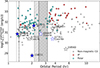 |
Fig. 11. Absorption-corrected X-ray luminosity (0.5–7 keV)–orbital period diagram for known CVs from the Ritter & Kolb (2003) catalog. X-ray luminosities were computed from fluxes in the ROSAT source catalog (2RXS) and distances in Gaia DR3. Circles represent CVs: known IP (red), polars (green), and nonmagnetic (gray). Vertical lines indicate the period minimum for CVs from Gänsicke et al. (2009, ≈82 min, dashed line) and Knigge (2006, ≈76 min, dotted line). The gray shaded regions show the CV orbital period gap from Schreiber et al. (2024, ≈2.5 − 3.2 h); and Knigge (2006, ≈2.2 − 3.2 h). The star markers denote new spectroscopically confirmed CVs (blue) and their candidates (white) from Table 1. We present two cases (Case A and Case B) for 2CXO J044048.3+292434 and 2CXO J173118.6+224248 as we cannot distinguish between the two orbital periods with our current data. For more details, see Sect. 5. |
5.1.3. 2CXO J123727.5+655211, a new polar
In Fig. 4 (top panels) we present the long-term ZTF light curve and the phase-folded light curve at the best period for 2CXO J123727.5+655211 (hereafter J12372). The ZTF light curve reveals a significant period at 2.12 h. The color dependence of cyclotron beaming is evident, with the ZTF i filter showing the highest modulation (peak-to-peak ∼2 mag) and the ZTF g filter showing the lowest (peak-to-peak ∼1 mag; see top left panel of Fig. 4).
We present the optical spectrum of J12372 in Fig. 4 (bottom panel). The spectrum shows hydrogen, helium, and high-excitation He II 4686 Å emission lines, yielding a line ratio of He II/Hβ ≈ 0.37 (see Table 3).
J12372 shows a flux ratio FX/Fopt ≈ 1.1 and an X-ray luminosity LX ≈ 4.4 × 1031 erg s−1 (see Table 1). The X-ray spectrum can be approximated by a power-law model with a photon index Γ ≈ 1.4 (or kT ≈ 38.3 keV for an optically thin thermal emission model) (see Table C.1 and Fig. C.1). X-ray timing analysis revealed no significant period in the longest exposure Chandra observation (see Table 4). J12372 shows significant X-ray flux variability (R ≈ 6; see Sect. 4.3), with a factor of ≈2 between the Chandra observations, but no statistically significant variability between the spectral parameters was found. J12372 lies close to the CV period gap in the X-ray luminosity–period diagram (see Fig. 10). Together with the optical light curves and spectrum, this indicates that J12372 is a polar.
5.1.4. 2CXO J182117.2–131405, low accretion rate polar
Figure 5 (top panels) shows the optical long-term ZTF light curve of 2CXO J182117.2–131405 (hereafter J18211) and the phase-folded light curve. We determined its best period to be 2.01 h using the Lomb–Scargle period analysis. The phase-folded optical light curve shows cyclotron beaming near phase 0.15 and ≈1 mag peak-to-peak modulation (see the top right panel of Fig. 5). This modulation could be either due to cyclotron beaming or to an eclipse of the WD by the donor star. High-speed photometry is needed to further investigate these scenarios.
J18211 has a low number of X-ray counts, and its spectrum can be approximately fitted by a power-law model, resulting in a large uncertainty for a photon index Γ ∼ 1.7 (or kT ≳ 1.6 keV for an optically thin thermal emission model) (see Table C.1 and Fig. C.1). J18211 shows a flux ratio FX/Fopt ≈ 0.15 and a lower X-ray luminosity (LX ≈ 6 × 1028 erg s−1) than typically seen in CVs (see Table 1). J18211 is located near the edge of the CV period gap in the X-ray luminosity–period diagram (see Fig. 10). In this part of the diagram, the canonical picture of CV evolution predicts that detached systems begin to undergo accretion again. Hence, J18211 could be a low accretion rate polar (previously referred to as a pre-polar).
We present the optical spectrum of J18211 in Fig. 5 (bottom panel). The spectrum is dominated by broad humps corresponding to cyclotron harmonics with no significant Hβ and He II 4686 Å emission lines detected. Using the equation for the electron gyration frequency around a magnetic field, we can define the wavelength of cyclotron harmonics as
 (2)
(2)
With the spacing of two harmonics, it is possible to constrain the magnetic field strength, as the spacing must always be the ratio of integers. We must assume a cyclotron beaming angle, which should be close to 90° since the amplitude of the cyclotron harmonics is so large. An angle θ > 60° is a good approximation for cyclotron beaming factors greater than 2 (e.g., Campbell et al. 2008). Detailed cyclotron modeling is beyond the scope of this paper. For this work we fixed the magnetic field at different values and approximately matched the location of the cyclotron humps in the spectrum to different cyclotron harmonics (see Fig. 5). This combination of the cyclotron wavelengths observed in the spectrum of J18211 and the large beaming amplitude constrains the magnetic field to be B ≈ 54 − 63 MG. This magnetic field strength is typical of low accretion rate polars (e.g., Parsons et al. 2021).
5.2. Variable CV candidates
Here, we discuss four CV candidates classified based on their X-ray and optical variability, but for which optical spectra are not yet available.
5.2.1. 2CXO J063805.1–801854, a possible magnetic CV
2CXO J063805.1–801854 (hereafter J06380) shows FX/Fopt ≈ 0.8 and X-ray luminosity LX ≈ 2.4 × 1031 erg s−1 (see Table 1). Its spectrum can be approximated by a power-law model with an unusually shallow photon index Γ ≈ 0.2 (or kT ≳ 75 keV for an optically thin thermal emission model; see Table C.1 and Fig. C.1). Such a shallow photon index is observed in the X-ray spectra of some magnetic CVs, such as polars or IPs (e.g., Galiullin & Gilfanov 2021). X-ray timing analysis revealed a ≈13 200 s periodicity (PF = 61%), which is consistent with the period previously found by Israel et al. (2016) in the same Chandra data (see Table 4 and Fig. 8). There is no available optical ZTF photometry for J06380. The Gaia optical light curve shows an outbursting-type variability with a ≈3 mag outburst lasting around ≈100 days and a possible recurrence time of approximately ≈500 days (see Fig. 6). Figure 10 shows that J06380 lies within main sample of known CVs. The X-ray periodicity (in the range of CV orbital periods), along with a high X-ray luminosity and hard spectrum, suggests that J06380 could be a magnetic CV, likely an IP.
5.2.2. 2CXO J165219.0–441401, a possible dwarf nova
2CXO J165219.0–441401 (hereafter J16521) shows FX/Fopt ≈ 1.2 and a high X-ray luminosity LX ≈ 3 × 1032 erg s−1 (see Table 1). The X-ray spectrum can be approximated by a power-law model with a photon index Γ ≈ 1.5 (or kT ≈ 5.8 keV for an optically thin thermal emission model; see Table C.1 and Fig. C.1). There is no ZTF photometry for J16521 and the Gaia optical light curve shows a ≈3 mag outburst with a possible ≈500-day recurrent time (see Fig. 6). This suggests that J16521 could be a dwarf nova.
5.2.3. 2CXO J173118.6+224248, a possible nonmagnetic CV
2CXO J173118.6+224248 (hereafter J17311) shows FX/Fopt ≈ 0.3 and an X-ray luminosity LX ≈ 2.4 × 1030 erg s−1 (see Table 1). The optical ZTF light curves show ≈0.5 mag variability with a period of about ≈1.8 h (see Fig. 2). However, the actual period may be twice this value, possibly due to ellipsoidal modulation. The X-ray spectrum can be approximated by a power-law model with a photon index Γ ≈ 2.2 (or kT ≈ 3.0 keV for an optically thin thermal emission model; see Table C.1 and Fig. C.1), a characteristic observed in nonmagnetic CVs. J17311 is located close to the main sequence of known CVs in the X-ray luminosity–orbital period diagram (see Fig. 10). The X-ray properties and optical variability suggest that J17311 is a nonmagnetic CV.
5.2.4. 2CXO J185603.2+021259, a possible eclipsing binary
2CXO J185603.2+021259 (hereafter J18560) shows FX/Fopt ≈ 0.05 and a lower X-ray luminosity (LX ≈ 2.5 × 1029 erg s−1) than observed in CVs (see Table 1). The ZTF optical light curve shows deep eclipses of approximately ≈1 mag in the r filter (or approximately ≈1.5 mag in the g filter) with a period of about 5.5 h (see Fig. 2). Out-of-eclipse sinusoidal variability of ≈0.1 mag is seen, possibly caused by the contribution from the donor. The X-ray spectrum can be approximated by a power-law model having a photon index Γ ≈ 2.8 (or kT ≈ 1 keV for an optically thin thermal plasma model; see Table C.1 and Fig. C.1). Figure 10 shows that J18560 is located below the main CV sample, similar to J18211. These observed properties suggest that J18560 could be an eclipsing binary.
6. Conclusions
We searched for new Galactic CV candidates among 25 887 sources in the CSC2, cross-matched them with Gaia DR3, and studied their optical and X-ray properties. We summarize our findings below:
-
We used a modern concept suggested by Rodriguez (2024) to classify new CVs among stellar objects based on a combination of FX/Fopt and Gaia BP–RP color (called the X-ray main sequence; see Fig. 1). We further defined a new threshold cut to compile a pure sample of CV candidates and minimize contamination from stellar objects (see Eq. 1 and Sect. 3).
-
We excluded known Galactic stellar objects by cross-matching the CSC2–Gaia DR3 catalog with the Simbad database and other publicly available CV catalogs (see Sect. 2). Out of 13 956 unclassified Galactic objects, we identified 14 new CV candidates using two different cuts on the X-ray main sequence (see Table 1 and Sect. 3).
-
All objects show X-ray luminosities in the range LX ≈ 1029 − 1032 erg s−1. Their X-ray spectra can be approximated by a power-law model with photon indices in the Γ ∼ 1 − 3 range or by an optically thin thermal emission model in the kT ∼ 1 − 70 keV range (see Fig. C.1 and Table C.1). These X-ray properties are mostly typical of CVs (both magnetic and nonmagnetic), but some objects might also be qLMXBs.
-
We performed optical follow-up observations with Keck I/LRIS and P200/DBSP and spectroscopically confirmed four objects as new CVs. Their optical spectra show prominent emission lines or cyclotron humps, typically seen in CVs (see Tables 2 and 3). We determined orbital periods for three of these objects using ZTF photometry. Among these, we discovered two polars, one low accretion rate polar and one nonmagnetic CV (WZ Sge type; see Sect. 5.1).
-
The X-ray and optical properties of four variable CV candidates suggest that three are potential magnetic systems or dwarf novae, while one may be an eclipsing binary (see Sect. 5.2). Further spectroscopic follow-up is required to confirm the nature of these objects.
Our analysis shows that a multiwavelength approach is a powerful tool for discovering new CVs and studying their properties. We illustrated that the X-ray main sequence presented in Rodriguez (2024) allows us to compile a sample of CV candidates for a detailed study. This approach can also be applied to other X-ray catalogs or upcoming all-sky SRG/eROSITA data to search for accreting binary systems. Further investigation of selection effects is necessary to use the X-ray main sequence to compile volume-limited samples of CVs and study their population.
For detailed flag descriptions see Evans et al. (2010) and CSC2 web-page: https://cxc.cfa.harvard.edu/csc/columns/flags.html
While creating the catalog of known systems, we had multiple matches (more than one) within the search radius for 810 of the 12 181 objects, giving about 7% of possible spurious associations in the catalog. However, for most objects with multiple matches a Simbad database provided a similar main object type (as defined in Table A.1). We adopted the Simbad object type from the nearest source for those objects.
Two periodic sources were already presented in the sample of 11 new CV candidates (selected by FX/Fopt and Gaia BP–RP color). Therefore, we added only three variable sources (out of five) in our final sample to include 14 CV candidates in total.
2CXO J044048.3+292434 was observed twice; both observations show equivalent width measurements that are in agreement to within 1σ. Therefore, in Table 3 we only report the values from the first exposure.
Such a binary would be an active binary, similar to RS CVn systems, which have orbital periods from as low as 5–6 hours to ∼10 days. In these systems X-rays originate from the hot corona of one or both stellar components (e.g., Walter & Bowyer 1981).
A two-component cyclotron model has been used to model the optical and near-infrared light curves of polars (e.g., Campbell et al. 2008). A two-component cyclotron model leads to two peaks in a single orbital period, and can be due to any of the following: two magnetic poles of different field strength, optical depth, and/or viewing angles.
We included this system in our analysis because it appears as an X-ray source (X) in Simbad, not explicitly as a CV.
Acknowledgments
This research has made use of data obtained from the Chandra Data Archive and software provided by the Chandra X-ray Center (CXC) in the application packages CIAO. This research has made use of the SIMBAD database, operated at CDS, Strasbourg, France. Based on observations obtained with the Samuel Oschin Telescope 48-inch and the 60-inch Telescope at the Palomar Observatory as part of the Zwicky Transient Facility project. ZTF is supported by the National Science Foundation under Grants No. AST-1440341 and AST-2034437 and a collaboration including current partners Caltech, IPAC, the Weizmann Institute of Science, the Oskar Klein Center at Stockholm University, the University of Maryland, Deutsches Elektronen-Synchrotron and Humboldt University, the TANGO Consortium of Taiwan, the University of Wisconsin at Milwaukee, Trinity College Dublin, Lawrence Livermore National Laboratories, IN2P3, University of Warwick, Ruhr University Bochum, Northwestern University and former partners the University of Washington, Los Alamos National Laboratories, and Lawrence Berkeley National Laboratories. Operations are conducted by COO, IPAC, and UW. The ZTF forced-photometry service was funded under the Heising-Simons Foundation grant No. 12540303 (PI: Graham). We are grateful to the staffs of the Palomar and Keck Observatories for their work in helping us carry out our observations. This work has made use of data from the European Space Agency (ESA) mission Gaia (https://www.cosmos.esa.int/gaia), processed by the Gaia Data Processing and Analysis Consortium (DPAC, https://www.cosmos.esa.int/web/gaia/dpac/consortium). Funding for the DPAC has been provided by national institutions, in particular the institutions participating in the Gaia Multilateral Agreement. This research made use of matplotlib, a Python library for publication quality graphics (Hunter 2007); NumPy (Harris et al. 2020); Astroquery (Ginsburg et al. 2019); Astropy, a community-developed core Python package for Astronomy (Astropy Collaboration 2013, 2018); and the VizieR catalogue access tool, CDS, Strasbourg, France. IG, AS, VD, NT acknowledge support from Kazan Federal University. ACR acknowledges support from the National Science Foundation via an NSF Graduate Research Fellowship. The authors thank the anonymous referee for useful and inspiring suggestions which helped to improve the manuscript.
References
- Abril, J., Schmidtobreick, L., Ederoclite, A., & López-Sanjuan, C. 2020, MNRAS, 492, L40 [NASA ADS] [CrossRef] [Google Scholar]
- Arnaud, K. A. 1996, ASP Conf. Ser., 101, 17 [Google Scholar]
- Astropy Collaboration (Robitaille, T. P., et al.) 2013, A&A, 558, A33 [NASA ADS] [CrossRef] [EDP Sciences] [Google Scholar]
- Astropy Collaboration (Price-Whelan, A. M., et al.) 2018, AJ, 156, 123 [Google Scholar]
- Bellm, E. C., Kulkarni, S. R., Graham, M. J., et al. 2019, PASP, 131, 018002 [Google Scholar]
- Boldin, P. A., Tsygankov, S. S., & Lutovinov, A. A. 2013, Astron. Lett., 39, 375 [NASA ADS] [CrossRef] [Google Scholar]
- Boller, T., Freyberg, M. J., Trümper, J., et al. 2016, A&A, 588, A103 [NASA ADS] [CrossRef] [EDP Sciences] [Google Scholar]
- Britt, C. T., Hynes, R. I., Johnson, C. B., et al. 2014, ApJS, 214, 10 [NASA ADS] [CrossRef] [Google Scholar]
- Campbell, R. K., Harrison, T. E., Schwope, A. D., & Howell, S. B. 2008, ApJ, 672, 531 [NASA ADS] [CrossRef] [Google Scholar]
- Cardelli, J. A., Clayton, G. C., & Mathis, J. S. 1989, ApJ, 345, 245 [Google Scholar]
- Cash, W. 1979, ApJ, 228, 939 [Google Scholar]
- Chambers, K. C., Magnier, E. A., Metcalfe, N., et al. 2016, ArXiv e-prints [arXiv:1612.05560] [Google Scholar]
- Chen, B. Q., Huang, Y., Yuan, H. B., et al. 2019, MNRAS, 483, 4277 [Google Scholar]
- Cordova, F. A., & Mason, K. O. 1984, MNRAS, 206, 879 [CrossRef] [Google Scholar]
- Cordova, F. A., Jensen, K. A., & Nugent, J. J. 1981, MNRAS, 196, 1 [Google Scholar]
- Dekany, R., Smith, R. M., Riddle, R., et al. 2020, PASP, 132, 038001 [NASA ADS] [CrossRef] [Google Scholar]
- DESI Collaboration (Adame, A. G., et al.) 2024, AJ, 168, 58 [NASA ADS] [CrossRef] [Google Scholar]
- DESI Collaboration (Aghamousa, A., et al.) 2016, ArXiv e-prints [arXiv:1611.00036] [Google Scholar]
- Downes, R. A., Webbink, R. F., Shara, M. M., et al. 2001, PASP, 113, 764 [Google Scholar]
- El-Badry, K., Conroy, C., Fuller, J., et al. 2022, MNRAS, 517, 4916 [NASA ADS] [CrossRef] [Google Scholar]
- Evans, I. N., Primini, F. A., Glotfelty, K. J., et al. 2010, ApJS, 189, 37 [NASA ADS] [CrossRef] [Google Scholar]
- Faulkner, J. 1971, ApJ, 170, L99 [NASA ADS] [CrossRef] [Google Scholar]
- Fruscione, A., McDowell, J. C., Allen, G. E., et al. 2006, SPIE Conf. Ser., 6270, 62701V [Google Scholar]
- Gaia Collaboration (Vallenari, A., et al.) 2023, A&A, 674, A1 [NASA ADS] [CrossRef] [EDP Sciences] [Google Scholar]
- Galiullin, I. I., & Gilfanov, M. R. 2021, Astron. Lett., 47, 587 [CrossRef] [Google Scholar]
- Galiullin, I., Rodriguez, A. C., Kulkarni, S. R., et al. 2024, MNRAS, 528, 676 [NASA ADS] [CrossRef] [Google Scholar]
- Gänsicke, B. T., Dillon, M., Southworth, J., et al. 2009, MNRAS, 397, 2170 [NASA ADS] [CrossRef] [Google Scholar]
- Ginsburg, A., Sipőcz, B. M., Brasseur, C. E., et al. 2019, AJ, 157, 98 [Google Scholar]
- Graham, M. J., Kulkarni, S. R., Bellm, E. C., et al. 2019, PASP, 131, 078001 [Google Scholar]
- Green, G. M., Schlafly, E., Zucker, C., Speagle, J. S., & Finkbeiner, D. 2019, ApJ, 887, 93 [NASA ADS] [CrossRef] [Google Scholar]
- Güver, T., & Özel, F. 2009, MNRAS, 400, 2050 [Google Scholar]
- Haberl, F., & Motch, C. 1995, A&A, 297, L37 [NASA ADS] [Google Scholar]
- Hameury, J. M. 2020, Adv. Space Res., 66, 1004 [Google Scholar]
- Harris, C. R., Millman, K. J., van der Walt, S. J., et al. 2020, Nature, 585, 357 [NASA ADS] [CrossRef] [Google Scholar]
- HI4PI Collaboration (Ben Bekhti, N., et al.) 2016, A&A, 594, A116 [NASA ADS] [CrossRef] [EDP Sciences] [Google Scholar]
- Hunter, J. D. 2007, Comput. Sci. Eng., 9, 90 [NASA ADS] [CrossRef] [Google Scholar]
- Inight, K., Gänsicke, B. T., Schwope, A., et al. 2023, MNRAS, 525, 3597 [NASA ADS] [CrossRef] [Google Scholar]
- Israel, G. L., Esposito, P., Rodríguez Castillo, G. A., & Sidoli, L. 2016, MNRAS, 462, 4371 [Google Scholar]
- Ivanova, N., Justham, S., Chen, X., et al. 2013, A&ARv, 21, 59 [Google Scholar]
- Jackim, R., Szkody, P., Hazelton, B., & Benson, N. C. 2020, Res. Notes Am. Astron. Soc., 4, 219 [Google Scholar]
- Khamitov, I. M., Bikmaev, I. F., Gilfanov, M. R., et al. 2023, Astron. Lett., 49, 271 [NASA ADS] [CrossRef] [Google Scholar]
- Knigge, C. 2006, MNRAS, 373, 484 [NASA ADS] [CrossRef] [Google Scholar]
- Knigge, C., Baraffe, I., & Patterson, J. 2011, ApJS, 194, 28 [Google Scholar]
- Kupfer, T., Korol, V., Littenberg, T. B., et al. 2024, ApJ, 963, 100 [NASA ADS] [CrossRef] [Google Scholar]
- Larsson, S. 1996, A&AS, 117, 197 [NASA ADS] [CrossRef] [EDP Sciences] [Google Scholar]
- Lazarz, D., Yan, R., Wilhelm, R., et al. 2022, A&A, 668, A21 [NASA ADS] [CrossRef] [EDP Sciences] [Google Scholar]
- Mackereth, J. T., Bovy, J., Leung, H. W., et al. 2019, MNRAS, 489, 176 [Google Scholar]
- Makarov, V. V., & Secrest, N. J. 2022, ApJ, 933, 28 [NASA ADS] [CrossRef] [Google Scholar]
- Maoz, D., Mannucci, F., & Nelemans, G. 2014, ARA&A, 52, 107 [Google Scholar]
- Masci, F. J., Laher, R. R., Rusholme, B., et al. 2019, PASP, 131, 018003 [Google Scholar]
- Merloni, A., Lamer, G., Liu, T., et al. 2024, A&A, 682, A34 [NASA ADS] [CrossRef] [EDP Sciences] [Google Scholar]
- NASA High Energy Astrophysics Science Archive Research Center (HEASARC) 2014, Astrophysics Source Code Library [record ascl:1408.004] [Google Scholar]
- Oke, J. B., & Gunn, J. E. 1982, PASP, 94, 586 [Google Scholar]
- Oke, J. B., Cohen, J. G., Carr, M., et al. 1995, PASP, 107, 375 [Google Scholar]
- Paczyński, B. 1967, Acta Astron., 17, 287 [NASA ADS] [Google Scholar]
- Paczynski, B. 1976, in Structure and Evolution of Close Binary Systems, eds. P. Eggleton, S. Mitton, & J. Whelan, 73, 75 [NASA ADS] [CrossRef] [Google Scholar]
- Parsons, S. G., Gänsicke, B. T., Schreiber, M. R., et al. 2021, MNRAS, 502, 4305 [CrossRef] [Google Scholar]
- Patterson, J. 1998, PASP, 110, 1132 [CrossRef] [Google Scholar]
- Perley, D. A. 2019, PASP, 131, 084503 [Google Scholar]
- Predehl, P., Andritschke, R., Arefiev, V., et al. 2021, A&A, 647, A1 [EDP Sciences] [Google Scholar]
- Pretorius, M. L., & Knigge, C. 2012, MNRAS, 419, 1442 [NASA ADS] [CrossRef] [Google Scholar]
- Prochaska, J., Hennawi, J., Westfall, K., et al. 2020, J. Open Source Softw., 5, 2308 [NASA ADS] [CrossRef] [Google Scholar]
- Queiroz, A. B. A., Anders, F., Chiappini, C., et al. 2020, A&A, 638, A76 [NASA ADS] [CrossRef] [EDP Sciences] [Google Scholar]
- Ramsay, G., Green, M. J., Marsh, T. R., et al. 2018, A&A, 620, A141 [NASA ADS] [CrossRef] [EDP Sciences] [Google Scholar]
- Rappaport, S., Verbunt, F., & Joss, P. C. 1983, ApJ, 275, 713 [Google Scholar]
- Ritter, H., & Kolb, U. 2003, A&A, 404, 301 [NASA ADS] [CrossRef] [EDP Sciences] [Google Scholar]
- Rodriguez, A. C. 2024, PASP, 136, 054201 [NASA ADS] [CrossRef] [Google Scholar]
- Rodriguez, A. C., Galiullin, I., Gilfanov, M., et al. 2023a, ApJ, 954, 63 [NASA ADS] [CrossRef] [Google Scholar]
- Rodriguez, A. C., Kulkarni, S. R., Prince, T. A., et al. 2023b, ApJ, 945, 141 [NASA ADS] [CrossRef] [Google Scholar]
- Schreiber, M. R., Zorotovic, M., & Wijnen, T. P. G. 2016, MNRAS, 455, L16 [NASA ADS] [CrossRef] [Google Scholar]
- Schreiber, M. R., Belloni, D., Gänsicke, B. T., Parsons, S. G., & Zorotovic, M. 2021, Nat. Astron., 5, 648 [NASA ADS] [CrossRef] [Google Scholar]
- Schreiber, M. R., Belloni, D., & Schwope, A. D. 2024, A&A, 682, L7 [NASA ADS] [CrossRef] [EDP Sciences] [Google Scholar]
- Schwope, A., Buckley, D. A. H., Kawka, A., et al. 2022a, A&A, 661, A42 [NASA ADS] [CrossRef] [EDP Sciences] [Google Scholar]
- Schwope, A., Buckley, D. A. H., Malyali, A., et al. 2022b, A&A, 661, A43 [NASA ADS] [CrossRef] [EDP Sciences] [Google Scholar]
- Smethurst, R. J., Masters, K. L., Simmons, B. D., et al. 2022, MNRAS, 510, 4126 [NASA ADS] [CrossRef] [Google Scholar]
- Souchay, J., Secrest, N., Lambert, S., et al. 2022, A&A, 660, A16 [NASA ADS] [CrossRef] [EDP Sciences] [Google Scholar]
- Sprague, D., Culhane, C., Kounkel, M., et al. 2022, AJ, 163, 152 [NASA ADS] [CrossRef] [Google Scholar]
- Spruit, H. C., & Ritter, H. 1983, A&A, 124, 267 [NASA ADS] [Google Scholar]
- Stone-Martinez, A., Holtzman, J. A., Imig, J., et al. 2024, AJ, 167, 73 [NASA ADS] [CrossRef] [Google Scholar]
- Sunyaev, R., Arefiev, V., Babyshkin, V., et al. 2021, A&A, 656, A132 [NASA ADS] [CrossRef] [EDP Sciences] [Google Scholar]
- Walter, F. M., & Bowyer, S. 1981, ApJ, 245, 671 [CrossRef] [Google Scholar]
- Warner, B. 2003, Cataclysmic Variable Stars (Cambridge: Cambridge University Press) [Google Scholar]
- Weisskopf, M. C., Tananbaum, H. D., Van Speybroeck, L. P., & O’Dell, S. L. 2000, SPIE Conf. Ser., 4012, 2 [Google Scholar]
- Weisskopf, M. C., Brinkman, B., Canizares, C., et al. 2002, PASP, 114, 1 [NASA ADS] [CrossRef] [Google Scholar]
- Wenger, M., Ochsenbein, F., Egret, D., et al. 2000, A&AS, 143, 9 [NASA ADS] [CrossRef] [EDP Sciences] [Google Scholar]
- Wevers, T., Torres, M. A. P., Jonker, P. G., et al. 2017, MNRAS, 470, 4512 [NASA ADS] [CrossRef] [Google Scholar]
- Wilms, J., Allen, A., & McCray, R. 2000, ApJ, 542, 914 [Google Scholar]
- Yang, H., Hare, J., Kargaltsev, O., et al. 2022, ApJ, 941, 104 [NASA ADS] [CrossRef] [Google Scholar]
Appendix A: General object types with a Simbad and FX/Fopt − (BP − RP) selection cut
Table A.1 shows our general object types based on the Simbad hierarchical structure. The columns are: (1) our main object type; (2) object subtype; (3) title of Simbad hierarchical structure used to define the main object type and its subtype; (4) number of sources per each object subtype, including known sources and their candidates. No source in our sample had an object type from the sixth Simbad’s hierarchy ("Gravitation"); therefore, it’s not shown in Table A.1.
Object types based on Simbad classification for 25,887 sources in the CSC2–Gaia DR3 catalog.
We investigated purity and completeness to construct a pure sample of new CV candidates and avoid contamination from stellar objects. Based on the Simbad hierarchical structure, we created two samples of known CVs (36 sources) and STARS (4781 sources; see Sect. 3.1).
Smethurst et al. (2022) computed purity and completeness for the red and blue galaxies classified by optical color. We applied a similar approach to define the purity and completeness as:
-
True positive (TP) = known CVs classified as CVs based on a given threshold (i.e., known CVs with an observed X-ray-to-optical ratio exceeding the threshold cut, (FX/Fopt)obs ≥ FX/Fopt)cut).
-
False positive (FP) = known STARS classified as CVs based on a given threshold (i.e., known STARS with an observed X-ray-to-optical ratio exceeding the threshold cut, (FX/Fopt)obs ≥ FX/Fopt)cut)).
-
False negative (FN) = known CVs classified as STARS (i.e., known CVs with an observed X-ray-to-optical ratio below the threshold cut, (FX/Fopt)obs < FX/Fopt)cut)).
Purity (P) is computed as the fraction of true identification to all identifications,
 (A.1)
(A.1)
and the completeness (C) is calculated as the fraction of true detections to all that should have been classified,
 (A.2)
(A.2)
To find the optimal combination of linear parameters (A, B) for Eq.1, we created a grid of parameters with the 0.1 steps in the range 0 ≲ A ≲ 3 and −8 ≲ B ≲ 3 and computed the purity and completeness.
Figure A.1 shows the purity and completeness as a function of linear parameters (A, B). For illustrative purposes, we show the purity and completeness only for three B parameters. The B = 0 case corresponds to the canonical selection cut based only on the X-ray-to-optical flux ratio without additional information from Gaia colors. For example, the cut FX/Fopt = 0.1 (where A = −1 and B = 0) gives ≈27% purity and ≈48% completeness. The drop of the purity above the A ≳ −0.2 is caused by a low number of sources and is not statistically significant. The Rodriguez (2024) empirical cut (A = −3.5 and B = 1) shows ≈25% purity and ≈78% completeness. In our study, we chose to use A = −1.5 and B = 0.7, which gives ≈100% purity and ≈52% completeness.
We note that our threshold is defined based only on a small sample of confirmed CVs (36 objects). To study the CV population and create a volume-limited sample, the FX/Fopt and Gaia BP–RP color diagram should be further investigated for selection effects with a large sample of confirmed CVs and stellar objects. A detailed investigation is beyond the scope of this paper.
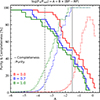 |
Fig. A.1. Purity (dotted line) and completeness (solid line) computed for different (A, B) parameters from Eq. 1. The vertical solid line corresponds to A = −1.5 (and B = 0.7), which is used to select a pure sample of CV candidates in this paper. The vertical dashed line shows A = −3.5 (and B = 1) for an empirical cut from Rodriguez (2024). |
Appendix B: Recently discovered CVs
We selected three objects from the CSC2–Gaia DR3 catalog using the X-ray main sequence as CV candidates (see Fig. 1 and Table B.1). In the course of this study, two of these objects (2CXO J024131.0+593630 and 2CXO J143435.3+334049) were recently discovered as CVs with SDSS spectra and ZTF light curves (Inight et al. 2023). Another object, 2CXO J174133.7–28403414, was confirmed as a CV via optical spectroscopy by Wevers et al. (2017). However, we included this object in our analyses to search for possible X-ray variability through timing and spectral analyses. Here, we individually discuss the X-ray and optical properties of these objects.
Previously known CVs independently found in our search of the CSC2–Gaia DR3 catalog.
 |
Fig. B.1. ZTF long-term light curves in g and r filters (left) and DBSP optical spectrum of 2CXO J024131.0+593630 (right). The gray lines represent the Keck Telluric Line List. The optical spectrum shows single-peaked hydrogen Balmer emission lines and a weak He II 4686Å emission line, giving a low line ratio He II/Hβ ≈ 0.12 (see Table B.2). Our analysis, based on optical and X-ray properties, suggests that J0241 is a new CV, likely nonmagnetic (see Sect. B.1 for more details). |
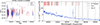 |
Fig. B.2. ZTF long-term (left) in g and r filters and the DBSP optical spectrum of 2CXO J143435.3+334049 (right). The gray lines represent the Keck Telluric Line List. The optical spectrum shows WD Balmer absorption lines with no sign of the donor signature in the optical spectrum and double-peaked, asymmetric Hα and Hβ emission lines. There is no detection of the high-excitation He II 4686Å emission line providing an upper limit for a line ratio He II/Hβ < 0.15 (see Table B.2). X-ray and optical properties suggest that the object is a low accretion rate CV (WZ Sge type; see Sect. B.2 for more details). |
B.1. 2CXO J024131.0+593630, a nonmagnetic CV
In the left panel of Fig. B.1, we present the long-term optical ZTF light curve of 2CXO J024131.0+593630 (hereafter J02413), which shows two significant (≈2 mag in r filter and ≈3 mag in g filter) short outbursts. A preliminary Lomb-Scargle period analysis reveals no periodicity in the ZTF and Gaia data, indicating that further observations are needed to determine the possible orbital period of this system.
We observed J02413 with P200/DBSP on 6 December 2023 for 900s. The optical spectrum of J02413 is presented in the right panel of Fig. B.1. Single-peaked hydrogen Balmer emission lines are clearly visible, and a weak He II 4686Å emission line is also present, giving a low line ratio He II/Hβ ≈ 0.12 (see Table B.2). However, as noted in Table B.2, the detection of He II 4686Å does not pass a visual inspection, so the value of the ratio should be interpreted as an upper limit. We also note that the detection (or nondetection) of He II 4686Å does not affect our final interpretation of this object.
J02413 shows a high flux ratio FX/Fopt ≈ 1.7 and an X-ray luminosity LX ≈ 1.5 × 1031 erg s−1 (see Table B.1). The X-ray spectrum of J02413 can be approximated by a power-law model with Γ ≈ 1.8 (or kT ≈ 5.5 keV for an optically thin thermal emission model; see Table C.1 and Fig. C.1). We found no significant period for J02413 from the X-ray timing analysis of the longest exposure Chandra observation (ObsID = 7152). J02413 also does not show X-ray flux variability and or changes in spectral parameters between observations. Our analysis, using optical and X-ray properties, suggests that J02413 is a CV, likely nonmagnetic. This agrees with Inight et al. (2023) conclusion, where J02413 is identified as a new nonmagnetic CV (U Gem type). The spectrum of this object is not shown in Inight et al. (2023), making our spectrum a useful addition to the literature.
Equivalent widths of selected lines of two previously known CVs.
B.2. 2CXO J143435.3+334049, a low accretion rate CV
In Fig. B.2 (left panel), we present the long-term ZTF light curve of 2CXO J143435.3+334049 (hereafter J14343). A preliminary Lomb-Scargle period analysis reveals no periodicity in the ZTF data, indicating that further observations are needed to determine the possible orbital period of this system.
We observed J14343 with P200/DBSP on 21 January 2023 for 900s. The optical spectrum of J14343 is presented in Fig. B.2 (right panel). The WD Balmer absorption lines are seen with double-peaked emission lines at the center, though the peaks appear to be asymmetric in height and width for both the Hα and Hβ lines. We do not detect the high-excitation He II 4686Å emission line providing an upper limit for a line ratio He II/Hβ < 0.15 (see Table B.2). There is no sign of the donor signature in the optical spectrum. The spectrum of this object in Fig. B.2 is different from the one shown in Inight et al. (2023), with the Balmer emission lines here being noticeably asymmetric. This could warrant future study of this system to further understand the nature of this source.
J14343 shows a flux ratio FX/Fopt ≈ 0.3 and a lower X-ray luminosity (LX ≈ 4.8 × 1029 erg s−1) than typically seen in CVs (see Table B.1). We have not detected statistically significant flux and spectral parameter variability between Chandra observations. The X-ray spectrum can be approximated by a power-law model with a photon index Γ ≈ 1.7 (or kT ≳ 5.2 keV for optically thin thermal emission model; see Table C.1 and Fig. C.1). X-ray and optical properties suggest that J14343 is a low accretion rate CV (WZ Sge type), similar to what Inight et al. (2023) concluded in their analysis.
B.3. 2CXO J174133.7–284034, a nonmagnetic CV
2CXO J174133.7–284034 (hereafter J17413 shows a flux ratio FX/Fopt ≈ 1.0 and an X-ray luminosity LX ≈ 4.4 × 1031 erg s−1 (see Table B.1). The X-ray spectrum of J17413 can be approximated by a power-law model with Γ ≈ 1.8 (or kT ≈ 5.6 keV for an optically thin thermal emission model; see Table C.1 and Fig. C.1). We have not detected statistically significant flux and spectral parameter variability between Chandra observations. We found no significant period for J17413 with the X-ray timing analysis for the longest exposure Chandra observation (ObsID = 9565). Britt et al. (2014) observed optical variability (≈1 mag) with no periodicity. Wevers et al. (2017) observed prominent emission lines and confirmed via optical spectroscopy that J17413 is a CV. Our X-ray analysis supports Britt et al. (2014) and Wevers et al. (2017) conclusions and also suggests that J17413 is likely a nonmagnetic system.
Appendix C: X-ray spectra figures
Figure C.1 shows Chandra X-ray spectra of all objects from Tables 1 and B.1. Table C.1 shows the results of the approximation of X-ray spectra with two spectral models: power-law (powerlaw in XSPEC with photon index parameter, Γ) and optically thin thermal plasma emission model (mekal in XSPEC with temperature kT, and metal abundance [Z] parameters).
Results of approximation of X-ray spectra of objects from Tables 1 and B.1 by different models.
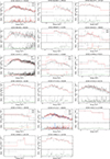 |
Fig. C.1. Chandra X-ray spectra of objects from Tables 1 and B.1 (top panel). The solid lines show the best-fit mekal model. The bottom panel shows the ratio of the data divided by the model in each energy channel. |
All Tables
Equivalent widths (−EW(Å)) of selected lines of four spectroscopically confirmed CVs.
Object types based on Simbad classification for 25,887 sources in the CSC2–Gaia DR3 catalog.
Previously known CVs independently found in our search of the CSC2–Gaia DR3 catalog.
Results of approximation of X-ray spectra of objects from Tables 1 and B.1 by different models.
All Figures
|
Fig. 1. X-ray-to-optical flux ratio vs Gaia (BP–RP) optical color (X-ray main sequence; Rodriguez 2024) for objects in the CSC2–Gaia DR3 catalog. Left panel: Known CVs (red) and stellar objects (STARS, blue) in the CSC2–Gaia DR3 catalog. The dashed black line shows an empirical cut from Rodriguez (2024). The solid red line shows a cut to select a pure sample of CV candidates. Right panel: Objects in the CSC2–Gaia DR3 catalog with the Simbad classifications (which may be imprecise). The colored symbols correspond to the different object types based on the Simbad hierarchical structure (see Table A.1). Objects above the solid red line and variable objects above the dashed black line are classified as new CV candidates (see Tables 1 and B.1). For more details, see Sect. 3. |
| In the text | |
|
Fig. 2. ZTF long-term (left) and phase-folded (right) light curves for 2CXO J173118.6+224248 (top panel) and 2CXO J185603.2+021259 (bottom panel) in g (blue) and r (red) filters. |
| In the text | |
|
Fig. 3. ZTF long-term (top left) and phase-folded (bottom left) light curves in g and r filters and the DBSP optical spectrum of 2CXO J044048.3+292434 (right). The gray lines represent the Keck Telluric Line List. The optical spectrum (top right) shows the hydrogen Balmer and helium emission lines and high-excitation He II 4686 Å emission line, giving a high line ratio He II/Hβ ≈ 0.64 (see Table 3). Optical and X-ray properties indicate that the object is a polar. Bottom right panel: Since two spectra taken 1.4 h apart do not show a significant radial velocity shift (a ≈ 1000 km/s shift would be expected if this were half of the orbital period and the system were viewed edge-on), the 1.3 h period is preferable. However, time-resolved spectroscopy for 2.6 h would be the only way to confirm the orbital period of this system, leading us to currently label the orbital period as either 1.3 or 2.6 h (see Sect. 5.1.1 for more details). |
| In the text | |
|
Fig. 4. ZTF long-term (top left) and phase-folded (top right) light curves in g, r, and i filters and the DBSP optical spectrum of 2CXO J123727.5+655211 (bottom). The gray lines represent the Keck Telluric Line List. The optical spectrum shows hydrogen, helium, and high-excitation He II 4686 Å emission lines, giving a line ratio of He II/Hβ ≈ 0.37 (see Table 3). Together with optical light curves, this indicates that the object is a polar (see Sect. 5.1.3 for more details). |
| In the text | |
|
Fig. 5. ZTF long-term (top left) and phase-folded (top right) light curves in g and r filters and the DBSP optical spectrum of 2CXO J182117.2–131405 (bottom). The gray lines represent the Keck Telluric Line List. The optical spectrum is dominated by broad humps that correspond to cyclotron harmonics, and no significant Hβ and He II 4686 Å emission lines are detected. A combination of the cyclotron wavelengths seen in the spectrum and the large beaming amplitude constrains the magnetic field to B ≈ 54 − 63 MG. Optical and X-ray properties suggest that the object is a low accretion rate polar (see Sect. 5.1.4 for more details). |
| In the text | |
|
Fig. 6. Gaia long-term light curves in G band for two sources in our sample. Panels: 2CXO J063805.1–801854 (left) and 2CXO J165219.0–441401 (right). |
| In the text | |
|
Fig. 7. X-ray and optical images for four new spectroscopically confirmed CVs from CSC2–Gaia DR3 catalog. Left: False-color Chandra X-ray images in the 0.5–7 keV energy band. The images were smoothed using a Gaussian kernel with different widths equal to 1 − 3 times the PSF radius, depending on the source counts. Right: Composite optical images based on Pan-STARRS i, r, and g filter data. The white boxes show the field of view of the optical images on the right. Circles: a PSF radius equal to the 90% of encircled counts fraction (solid white line), and a radius equal to the semimajor axis of the error ellipse (95% localization error) centered on the source X-ray position (dashed magenta line). |
| In the text | |
|
Fig. 8. ZTF long-term light curves in g and r filters (left) and DBSP optical spectrum of 2CXO J044147.9–015145 (right). The gray lines represent the Keck Telluric Line List. The optical spectrum shows WD Balmer absorption lines with no sign of the donor signature, weakly double-peaked hydrogen and helium emission lines, and no detectable He II 4686 Å emission line, giving a 3σ upper limit for the line ratio He II/Hβ < 0.05 (see Table 3). Optical and X-ray properties suggest that the object is a CV (WZ Sge type; see Sect. 5.1.2 for more details). |
| In the text | |
|
Fig. 9. Chandra X-ray pulse profile for 2CXO J063805–801854 normalized by mean count rate 0.01 cnt s−1. |
| In the text | |
|
Fig. 10. Extinction-corrected Hertzsprung-Russell (HR) diagram. All Gaia sources within 100 pc with significantly measured parallaxes (parallax_over_error > 3) are shown in gray (Gaia Collaboration 2023). The star markers represent new spectroscopically confirmed CVs (blue) and variable CV candidates (white) from Table 1. The white circles indicate CV candidates selected by a FX/Fopt ratio and Gaia (BP–RP) color: (1) J165219.0–441401; (2) J173332.5–181735; (3) J094607.7–311550; (4) J155926.5–754311; (5) J190823.2+343328; (6) J173555.3–292530. |
| In the text | |
|
Fig. 11. Absorption-corrected X-ray luminosity (0.5–7 keV)–orbital period diagram for known CVs from the Ritter & Kolb (2003) catalog. X-ray luminosities were computed from fluxes in the ROSAT source catalog (2RXS) and distances in Gaia DR3. Circles represent CVs: known IP (red), polars (green), and nonmagnetic (gray). Vertical lines indicate the period minimum for CVs from Gänsicke et al. (2009, ≈82 min, dashed line) and Knigge (2006, ≈76 min, dotted line). The gray shaded regions show the CV orbital period gap from Schreiber et al. (2024, ≈2.5 − 3.2 h); and Knigge (2006, ≈2.2 − 3.2 h). The star markers denote new spectroscopically confirmed CVs (blue) and their candidates (white) from Table 1. We present two cases (Case A and Case B) for 2CXO J044048.3+292434 and 2CXO J173118.6+224248 as we cannot distinguish between the two orbital periods with our current data. For more details, see Sect. 5. |
| In the text | |
|
Fig. A.1. Purity (dotted line) and completeness (solid line) computed for different (A, B) parameters from Eq. 1. The vertical solid line corresponds to A = −1.5 (and B = 0.7), which is used to select a pure sample of CV candidates in this paper. The vertical dashed line shows A = −3.5 (and B = 1) for an empirical cut from Rodriguez (2024). |
| In the text | |
|
Fig. B.1. ZTF long-term light curves in g and r filters (left) and DBSP optical spectrum of 2CXO J024131.0+593630 (right). The gray lines represent the Keck Telluric Line List. The optical spectrum shows single-peaked hydrogen Balmer emission lines and a weak He II 4686Å emission line, giving a low line ratio He II/Hβ ≈ 0.12 (see Table B.2). Our analysis, based on optical and X-ray properties, suggests that J0241 is a new CV, likely nonmagnetic (see Sect. B.1 for more details). |
| In the text | |
|
Fig. B.2. ZTF long-term (left) in g and r filters and the DBSP optical spectrum of 2CXO J143435.3+334049 (right). The gray lines represent the Keck Telluric Line List. The optical spectrum shows WD Balmer absorption lines with no sign of the donor signature in the optical spectrum and double-peaked, asymmetric Hα and Hβ emission lines. There is no detection of the high-excitation He II 4686Å emission line providing an upper limit for a line ratio He II/Hβ < 0.15 (see Table B.2). X-ray and optical properties suggest that the object is a low accretion rate CV (WZ Sge type; see Sect. B.2 for more details). |
| In the text | |
|
Fig. C.1. Chandra X-ray spectra of objects from Tables 1 and B.1 (top panel). The solid lines show the best-fit mekal model. The bottom panel shows the ratio of the data divided by the model in each energy channel. |
| In the text | |
Current usage metrics show cumulative count of Article Views (full-text article views including HTML views, PDF and ePub downloads, according to the available data) and Abstracts Views on Vision4Press platform.
Data correspond to usage on the plateform after 2015. The current usage metrics is available 48-96 hours after online publication and is updated daily on week days.
Initial download of the metrics may take a while.