| Issue |
A&A
Volume 690, October 2024
|
|
|---|---|---|
| Article Number | A381 | |
| Number of page(s) | 10 | |
| Section | The Sun and the Heliosphere | |
| DOI | https://doi.org/10.1051/0004-6361/202450714 | |
| Published online | 24 October 2024 | |
Derivation of a generalized Kappa distribution from the scaling properties of solar wind magnetic field fluctuations at kinetic scales
1
Department of Physics, University of Rome Tor Vergata, Via della Ricerca Scientifica 1, Rome 00133, Italy
2
INAF – Institute for Space Astrophysics and Planetology, Via del Fosso del Cavaliere 100, Rome 00133, Italy
⋆⋆ Corresponding author; simone.benella@inaf.it
Received:
14
May
2024
Accepted:
2
September
2024
Context. Kinetic-scale dynamics in weakly collisional space plasmas usually exhibits a self-similar statistics of magnetic field fluctuations. This implies the existence of an invariant probability density function (master curve).
Aims. We provide an analytical derivation of the master curve by assuming that perpendicular fluctuations can be modeled through a scale-dependent Langevin equation.
Methods. In our model, magnetic field fluctuations are the stochastic variable, and their scale-to-scale evolution is assumed to be a Langevin process. We propose a formal derivation of the master curve describing the statistics of the fluctuations at kinetic scales. The model predictions were tested on independent data samples of the fast solar wind measured near the Sun by Parker Solar Probe and near the Earth by Cluster.
Results. The master curve is a generalization of the Kappa distribution with two parameters: One parameter regulates the tails, and the other controls the asymmetry. The model predictions match the spacecraft observations up to 5σ and even beyond in the case of perpendicular magnetic field fluctuations.
Key words: magnetic fields / turbulence / waves / Sun: heliosphere / solar wind
© The Authors 2024
 Open Access article, published by EDP Sciences, under the terms of the Creative Commons Attribution License (https://creativecommons.org/licenses/by/4.0), which permits unrestricted use, distribution, and reproduction in any medium, provided the original work is properly cited.
This article is published in open access under the Subscribe to Open model. Subscribe to A&A to support open access publication.
1. Introduction
In the context of space and astrophysical plasmas, which encompass environments such as solar and stellar winds, planetary magnetospheres, and the interstellar medium, the dynamic interplay of energy fluctuations that are related to various physical processes unfolds across an extensive range of spatial and temporal scales. Diverse structures, including current sheets, plasmoids, and vortices, emerge as a consequence (Coleman 1968; Higdon 1984; Zhuravleva et al. 2014). Large-scale velocity and magnetic field fluctuations, where plasma behaves like a single fluid, show the typical hallmarks of fully developed turbulence (Belcher & Davis 1971; Biskamp 2003). Conversely, at scales smaller than the characteristic ion length (kinetic scales) where the motion of ions and electrons decouples, the interaction between different kinetic processes yields fluctuations with distinct spectral and statistical features (Cranmer & van Ballegooijen 2003; Bale et al. 2005; Chen et al. 2013; Bruno & Carbone 2016). Space missions have provided solar wind observations with an increasingly higher resolution over the past decades and still continue to do this. This enabled us to investigate the statistical properties of the magnetic field fluctuations from the fluid to the ion-kinetic regime (Chasapis et al. 2017; Chhiber et al. 2021).
In the attempt to understand the dynamics at kinetic scales in the solar wind, statistical methods have emerged as indispensable tools because they are closely related to fundamental physical quantities, such as the energy transfer, and they are the subject of theoretical predictions (Bruno & Carbone 2016). In turbulence, for example, the careful examination of the common statistical properties that are shared by flows in diverse systems, from fluids to laboratory and space plasmas, introduced the concept of universality (L’Vov 1998; Frisch 1995; Arnèodo et al. 2008). The idea of universality consists of the emergence of common statistical properties (e.g., scaling exponents and spectral slope) in a large set of independent data samples, indicating that statistical laws emerge regardless of the specific processes underlying energy injection or dissipation. In the case of space plasma turbulence, for instance, the emergence of a power law in the power spectra of velocity and magnetic fields, E(f)∼f−α as a function of frequency, is ubiquitous in spacecraft data, with α very close to 5/3 or 3/2 at inertial scales (i.e., at scales larger than the ion inertial length and smaller than the correlation length), in agreement with the predictions by Kolmogorov (1941) and Kraichnan (1965). Conversely, the scaling exponents of the spectral density that are routinely observed at kinetic scales do not show universal values and are therefore strongly dependent on the considered data sample (Sahraoui et al. 2013; Carbone et al. 2022; Sahraoui & Huang 2023). This suggests that at scales smaller than the ion inertial length, there is a transition towards a dynamical regime that is formed by processes of different nature with respect to the magnetohydrodynamic turbulence. The search for universal properties in this range would be important in order to test whether even kinetic-scale physics is characterized by the emergence of universal dynamics. However, universality is to be sought elsewhere because spectral exponents do not exhibit this property. In contrast to what is expected for a turbulent plasma, one of the striking features of kinetic scale dynamics that was highlighted from several data samples in both spacecraft measurements and numerical simulations is the self-similar statistics of magnetic field fluctuations, which implies the existence of a scale-invariant probability density function, the so-called master curve, in this range of scales (see, e.g., Consolini et al. 2005; Kiyani et al. 2009; Osman et al. 2015; Leonardis et al. 2016). Theoretical frameworks able to describe such properties and provide mathematical models for probability distribution functions (PDFs), scaling exponents, and so on, are therefore of primary importance in the search for universal behaviors at small scales. Among these, methods based on stochastic process theory are very effective in capturing and predicting the statistical properties of fluctuating time series (e.g, see the book Tabar 2019).
Descriptions of turbulent and kinetic dynamics based on stochastic processes have recently emerged in the field of astrophysical plasmas such as the solar photosphere (Asensio Ramos & Martínez González 2014; Gorobets et al. 2016), the solar wind (Strumik & Macek 2008; Carbone et al. 2021, 2022; Bian & Li 2022; Benella et al. 2022a; Bian & Li 2024a,b) and the Earth magnetosheath (Macek et al. 2023; Chiappetta et al. 2023; Macek & Wójcik 2023; Wójcik & Macek 2024). Many of these models are designed to predict PDFs and infer stochastic equations governing the fluctuations at different scales, thereby extending earlier findings from fluid turbulence (e.g., see Friedrich & Peinke 1997; Renner et al. 2001) to space plasmas. In the case of plasmas, both velocity and magnetic field increments at different scales can be envisioned as Langevin processes, in which the physics of the evolution and interaction of structures is enclosed within stochastic diffusion terms. The statistics of these processes offer a description that is equivalent to scaling models when the drift and diffusion terms are chosen appropriately (Nickelsen 2017; Friedrich & Grauer 2020). In this context, the aim of this work is to use the generalized Langevin equation to formally derive a master curve representative of the magnetic field fluctuations that are observed in space plasmas at kinetic scales. The derivation of an analytical expression for this distribution may be important in the search for new universal properties of kinetic-scale fluctuations. As we show, the PDF can be expressed as a Kappa distribution. Kappa distributions play a fundamental role in the field of space plasmas (Livadiotis 2017; Lazar & Fichtner 2021). Empirically introduced by Olbert (1968) and Vasyliunas (1968) to model electron fluxes observed by early space missions, these distributions have led to significant advancements in understanding and modeling space plasma dynamics related to various fundamental mechanisms such as particle acceleration (Zank et al. 2006; Fisk & Gloeckler 2014; Bian et al. 2014), turbulence (Leubner & Vörös 2005; Yoon 2012, 2014; Gravanis et al. 2019; Yoon 2020), systems in which the temperature, or other relevant thermodynamic quantities, vary according to a certain distribution and are not constant (i.e., superstatistics; Beck & Cohen 2003; Schwadron et al. 2010; Livadiotis 2019; Gravanis et al. 2020), or pick-up ion cooling (Livadiotis et al. 2012, 2024). Kappa distributions are particularly effective in describing different plasma populations in the heliosphere (Collier et al. 1996; Maksimovic et al. 1997; Pierrard et al. 1999; Mann et al. 2002; Marsch 2006; Zouganelis 2008; Livadiotis & McComas 2010; Pavlos et al. 2016; Livadiotis 2017; Lazar & Fichtner 2021).
Focusing on solar wind magnetic field fluctuations at kinetic scales, we aim to derive the Kappa distribution from the scaling properties of the magnetic field. To do this, we summarize in Section 2 some relevant scaling theories of turbulence and to highlight their connection with the Langevin description. In Section 3 we illustrate the solution of the associated stationary Fokker–Planck equation (FPE), which leads to the Kappa distribution. In Section 4 we test the predictions of our model against solar wind data, and in Section 5 we draw our conclusions.
2. Stochastic model for magnetic field increments
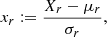
In magnetohydrodynamic turbulence, it is common practice to use velocity/magnetic field increments as a proxy of the amount of energy that is contained at a given scale r into the system. As the energy is transferred from the injection scales toward dissipative scales, the amount of energy, and thus the level of fluctuations, decreases for decreasing r. Statistical analysis involves high-order moments of increments Xr of a field F, defined as

at a scale separation r. If these increments exhibit a global scale invariance, large structures divide into increasingly smaller structures. When this process is homogeneous, each structure decays in the same manner and the field F is said to be globally self-similar or globally scale invariant. Formally, the global invariance can be expressed as
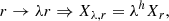
where h is the scaling exponent, and λ ∈ ℝ+ is a dilation parameter. This results in the power-law behavior of the individual realization Xr of the process and of the structure functions, Sq(r)∼rζq, with ζq as the scaling exponents. The self-similarity hypothesis was part of the first theory proposed by Kolmogorov (1941). In particular, he proposed the linear relation for the scaling exponents ζq = q/3, where q indicates the order of the moment. In this context, ζq signifies how increments at different scales contribute to the overall statistical behavior of turbulence. Given the fluctuation level Xr at the scale r, a simple choice accounting for the subtraction of energy in a self-similar way is represented by the damping equation,

where the drift term depends on the scale r and the process Xr. When we assume that m(r)∼h r−1, the solution of the damping equation is a power law,
Despite its simplicity, which makes it unsuitable for describing a typical turbulent dynamics, it has recently been pointed out that the damping trend may constitute a reasonable zeroth-order approximation of kinetic scale fluctuations in the solar wind (Benella et al. 2023). Nevertheless, Equation (4) produces deterministic trajectories that behave as power laws with a unique exponent h, whereas the typical dynamics of the magnetohydrodynamic regime is richer and chaotic, and it typically exhibits a set of h that depends on space and on the separation scale (Parisi et al. 1985; Frisch 1995). As a result, the scaling exponent ζq of the structure functions is a nonlinear function of the order q. This statistical signature is known as anomalous scaling, which is directly related to intermittency and which has been captured through a plethora of statistical models, for example, log-normal scaling, which is also known as the refined similarity hypothesis by Kolmogorov in 1962 (K62; Kolmogorov 1962; Obukhov 1962), a log-Poisson model (Dubrulle 1994), te She-Leveque model (She & Leveque 1994), random cascade models (Castaing & Dubrulle 1995), the Yakhot model (Yakhot 1998), and so forth. In terms of the energy cascade mechanism, intermittency is related to nonhomogeneity of the energy transfer/dissipation rate, that is, the efficiency of the energy cascade depends on space and time.
In the context of a stochastic description of the changing fluctuations across the scales, we can introduce a stochastic term that is characterized by pure multiplicative noise in Equation (4). This leads to a real Itô stochastic process that is defined through a generalized Langevin equation,
where Wr is a standard Wiener process with zero mean and unit variance, and D(Xr, r) = D(Xr) = αXr2/2 is the diffusion term1. The formal solution of Equation (5) is
Therefore, at an individual level, we ultimately have a stochastic variable driven by the Wiener process Wr. Moreover, since Wr is normally distributed, Equation (5) implies that Xr must follows a log-normal distribution, thus resembling, for instance, the K62 correction to scaling (Kolmogorov 1962; Obukhov 1962). From the perspective of a stochastic process, the log-normal scaling represents the easiest way to introduce stochasticity in the fluctuations and thus in the transfer of energy at the individual level (Nickelsen 2017; Fuchs et al. 2022). Nevertheless, a general second-order polynomial function can introduce interesting and more realistic features, for instance, additive noise over multiplicative noise, which resemble empirical observations at the cost of the simplicity of providing a formal solution to the stochastic differential equation with respect to the log-normal hypothesis (see Reinke et al. 2018, for further details). For the sake of generality, we thus introduce a first-order polynomial L and a second-order polynomial Q,


where Q0 > 0 and 4Q0Q2 > Q12, and we assume, when explicit computation is needed, that M ≡ L and D ≡ Q.
3. Analytical derivation of the master curve
In the case of the Langevin process, the probability density ρr(X) of finding Xr in the state X satisfies the FPE, which is thus the master equation of the process (Risken 1996)
![$$ \begin{aligned} \frac{\partial \rho _r(X)}{\partial r} = \frac{\partial }{\partial X}\biggl [\frac{\partial }{\partial X}(D(X,r)\rho _r(X)) - M(X,r)\rho _r(X)\biggr ]. \end{aligned} $$](/articles/aa/full_html/2024/10/aa50714-24/aa50714-24-eq9.gif)
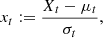
When we consider the standardized process
where μr and σr are the scale-dependent mean value and standard deviation, the probability density pr(x) of finding xr at x is given by

and satisfies the FPE with drift and diffusion terms
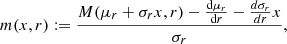
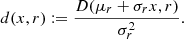
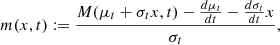
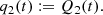
By choosing M ≡ L and D ≡ Q, we obtain m ≡ l and d ≡ q, where
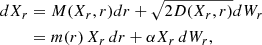
![$$ \begin{aligned} l(x,r)&:= - [q_0(r) + q_2(r)]x,\end{aligned} $$](/articles/aa/full_html/2024/10/aa50714-24/aa50714-24-eq14.gif)

The set of parameters {q0, q1, q2} refers to the drift and diffusion terms of the standardized variable and can be expressed in terms of the parameters {Q0, Q1, Q2} of Equation (8) as
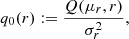
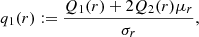
The evolution of the stochastic process (Eq. (5)) as a function of the scales therefore also implies a FPE for the standardized variable xr. This equation, with linear drift and quadratic diffusion, cannot be solved analytically without further hypotheses. Since the statistics of kinetic scales in the solar wind is observed to be monofractal, this implies that the probability density functions can be recast on a master curve by simply rescaling the variable with the standard deviation σr (Consolini et al. 2005; Kiyani et al. 2009; Osman et al. 2015; Benella et al. 2022a). In this spirit, we assumed the stationary condition of the standardized process (xr)r ≥ 0, that is, ∂pr/∂r ≡ 0, and we obtain the following analytical solution for the FPE:
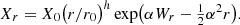
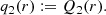
![$$ \begin{aligned} p_{\kappa ,\lambda }(x) = N_{\kappa ,\lambda }\biggl [1 + \frac{1}{\kappa }\frac{(x - \lambda )^2}{x_{\kappa ,\lambda }^2}\biggr ]^{-\kappa -1}\exp \biggl (- \frac{2\lambda \sqrt{\kappa }}{x_{\kappa ,\lambda }}\tan ^{-1}\biggl (\frac{x - \lambda }{\sqrt{\kappa }x_{\kappa ,\lambda }}\biggr )\biggr ), \end{aligned} $$](/articles/aa/full_html/2024/10/aa50714-24/aa50714-24-eq19.gif)
where
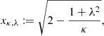
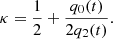
with i being the imaginary unit and Γ the Euler gamma function, and
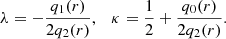
For a detailed formal derivation of these equations we refer to Appendix A. We note that 2κ > 1 + λ2 by construction. In particular, for λ = 0, we obtain the familiar Kappa distribution
The obtained stationary distribution (Eq. (23)) corresponds to the Kappa distribution, and for this reason, we refer to Equation (19) as the generalized Kappa distribution. We emphasize that the obtained Kappa distribution represents the probability measure of one-dimensional stochastic process xr and should not be confused with the conventional Kappa distribution in the velocity space defined in three dimensions (Olbert 1968; Vasyliunas 1968; Lazar & Fichtner 2021). The distribution (Eq. (19)) depends on two parameters: the shape parameter κ, which regulates the weight of the tails of the distribution, for instance, tending toward a Gaussian for κ → ∞ in Equation (23), and the symmetry parameter λ, representing an important and innovative generalization of a Kappa distribution, allowing the distribution to be asymmetric with respect to zero. A sketch of the stationary distribution (Eq. (19)) for three different values of the parameter λ = −0.2, 0, 0.2 and κ = 1 is illustrated in Figure 1. As long as the parameter λ is equal to zero, the distribution is symmetric. Conversely, when this parameter is positive/negative, one of the tails of the distribution tends to be higher than the other, thus producing nonvanishing odd moments (e.g., nonvanishing skewness). For the first- and second-order moments, we have
 |
Fig. 1. Example of a stationary distribution (Eq. (19)) with κ = 1 for different values of λ. The dashed line indicates λ = −0.2, the dotted line shows λ = 0.2, and the solid line shows the Kappa distribution (Eq. (23)). |
regardless of the values of κ and λ (provided 2κ > 1 + λ2), as required for the random variable xr in Eq. (10), by construction.
To summarize, when we consider a stochastic process Xr of the Langevin type defined by the drift and diffusion terms of Equations (7) and (8), the solution is the generalized Kappa distribution (Eq. (19)) when the density function pr(x) of the standardized process xr is stationary.
4. Results
In order to test these analytical results on spacecraft observations, we defined the longitudinal increment of the interplanetary magnetic field as ![$ b_r:=[\boldsymbol{B}(\boldsymbol{x}+\boldsymbol{r})-\boldsymbol{B}(\boldsymbol{x})]\cdot\hat{\boldsymbol{r}} $](/articles/aa/full_html/2024/10/aa50714-24/aa50714-24-eq25.gif) , where B is the magnetic field vector, and r is the separation vector between the two measurements. This quantity is our stochastic variable br ≡ Xr, and the variation of br as a function of the scale separations r defines a stochastic process. We considered two independent data samples of fast solar wind streams at different heliocentric distances as a test for the model introduced in the previous section. We describe the two samples below.
, where B is the magnetic field vector, and r is the separation vector between the two measurements. This quantity is our stochastic variable br ≡ Xr, and the variation of br as a function of the scale separations r defines a stochastic process. We considered two independent data samples of fast solar wind streams at different heliocentric distances as a test for the model introduced in the previous section. We describe the two samples below.
-
The first sample is an Alfvénic fast wind data interval gathered by the FIELDS suite (Bale et al. 2016) on board Parker Solar Probe (PSP) during its first perihelion between 02:00 UT and 04:00 UT on 2018 November 9 at a heliocentric distance of approximately 0.17 au. We used the merged fluxgate and search-coil magnetometers (SCaM) magnetic field data product. It is available with a time resolution of 146.5 samples/s (Bowen et al. 2020).
-
The second data sample was measured during a fast wind stream by the Cluster 3 (C3) spacecraft in the near-Earth environment, ∼1 au, between 12:00 UT and 14:00 UT on 2007 January 20 (Yordanova et al. 2015; Alberti et al. 2019). High-cadence magnetic field data were obtained by the merged measurements of fluxgate magnetometer (FGM) (Balogh et al. 1997) and spatio-temporal analysis of field fluctuations (STAFF) (Cornilleau-Wehrlin et al. 1997) instruments, reaching a time resolution of 450 samples/s.
More details of the average bulk plasma parameters related to the data samples selected for this study are summarized in Table 1.
Bulk solar wind parameters for the data samples.
The data used in this work are reported in Figure 2. To infer information about the spatial increment vector b = B(x + r)−B(x), we assumed that the Taylor hypothesis is valid. This hypothesis requires that the Alfvén velocity, which represents the fastest propagating perturbation in plasmas, must be lower than the flow speed. The average values of the Alfvén velocity are reported in Table 1. If V is the average flow speed, the timescale separation τ can be converted into the spatial separation vector through the relation r = Vτ, which fixes the sampling direction parallel to the solar wind velocity. The solar wind expands almost radially, and we therefore selected the radial component of both magnetic field data samples, that is, BR for PSP and the x component in the Geocentric Solar Ecliptic (GSE) reference frame for C3, as representative of the sampling direction, since C3 is in the Earth orbit. The power spectral densities of the two data samples we used in the analysis are presented in Figure 3. Typical spectral slopes of fully developed turbulence, that is, a Kolmogorov spectrum f−1.7, and kinetic scale fluctuations, with a steeper trend f−α, with α ∈ [2.5, 2.7], are reported for reference. The spectral frequency associated with the smallest scale used in the analysis is indicated by the vertical blue line, corresponding to τ = 0.020 s for PSP and τ = 0.027 s for C3. The Doppler-shifted frequencies associated with the ion inertial length fd = V/(2πdi) and ion gyroradius fρ = V/(2πρi) are also reported in the figure. By virtute of Taylor’s hypothesis, temporal scales can be interpreted as spatial scales and vice versa.
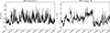 |
Fig. 2. Radial component of the magnetic field BR observed by PSP during the first perihelion (left), and magnetic field component Bx in the GSE coordinate system observed by the C3 spacecraft (right). |
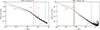 |
Fig. 3. Power spectral density of the 2018 November 9 PSP data interval (left) and of the 2007 January 20 C3 data sample (right). Vertical lines indicate frequencies associated with the ion inertial length (red) and the ion gyroradius (green). The blue lines indicate the smallest scales considered in the analysis. The typical slopes in the inertial and kinetic ranges are reported for reference (dotted lines). |
The magnetic field fluctuations developed by turbulence and kinetic-scale dynamics in the solar wind are inherently anisotropic (Horbury et al. 2012). The presence of a strong outward/inward mean field generated by the Sun sets a preferential direction in space that tends to inhibit strong parallel fluctuations. As a result, magnetic field fluctuations develop more intensely in the direction perpendicular to the magnetic field. We defined the local mean magnetic field as
![$$ \begin{aligned} \boldsymbol{B}_{loc}(s, t) = A_s \sum _{k=1}^{N} \boldsymbol{B}(t_k)\exp {\left[\frac{-(t_k - t)^2}{2s^2}\right]} , \end{aligned} $$](/articles/aa/full_html/2024/10/aa50714-24/aa50714-24-eq26.gif)
where s indicates the scale and As the normalization constant,
![$$ \begin{aligned} A_s^{-1} = \sum _{k=1}^{N} \exp {\left[\frac{-(t_k - t)^2}{2s^2}\right]}, \end{aligned} $$](/articles/aa/full_html/2024/10/aa50714-24/aa50714-24-eq27.gif)
and we estimated the angle θVB(x, r) with respect to the sampling direction (Horbury et al. 2008; Podesta 2009; Podesta & Gary 2011). We emphasize that this particular choice for defining the mean local magnetic field does not affect the results. We verified that the use of different prescriptions, such as the moving average of the magnetic field vector with a window of length 102di, did not affect the results significantly (not shown). We only considered fluctuations perpendicular to Bloc by introducing the condition 80° < θVB < 100° in the magnetic field increments b. The histograms of the angles θVB observed in the PSP and C3 data samples are shown in Figure 4. We note that the probability density associated with perpendicular fluctuations, that is, between the vertical lines, in the case of C3 is slightly higher than in the PSP data interval. The scale at which the statistics is displayed is τ = 0.03 s, but it is representative of the overall angle statistics due to the weak scale dependence of the probability density shown in Figure 4 (not shown).
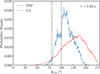 |
Fig. 4. Histograms of the angle θVB between the local mean magnetic field and the sampling direction for the PSP and C3 data samples. The statistics have been calculated at scale τ = 0.03 s, and the vertical lines delineate the region 80° < θVB < 100° around the perpendicular direction. |
The first step in the analysis was to estimate the scale-by-scale parameters κ and λ defined in Equation (22). These equations rely on the parameterization of the function D, which is assumed to be a quadratic polynomial Q(br, r). This assumption, justified in Section 2 as a rather general choice in order to describe turbulent fluctuations in terms of an advection/diffusion dynamics, constitutes well-documented empirical evidence in the small scales of the solar wind Benella et al. (2022a,b). By using magnetic field observations, we estimated all the scale-dependent parameters {Q0, Q1, Q2} appearing in Equations (7) and (8) by fitting the Kramers–Moyal (KM) coefficients D(br, r) scale by scale. This iterative procedure provides the entire set of functions DΔ(br, r) representing the finite-scale approximations of the true second-order KM coefficient D(br, r), where Δ indicates the small step used in the calculation. Therefore, when we use Equation (15) in order to link the set of parameters {Q0, Q1, Q2} to the parameters {q0, q1, q2} of the standardized fluctuation br, we must take the correction terms arising from the finite-scale approximation into account (Benella et al. 2022b). Further details on the correct estimation of finite-scale KM coefficients are reported in Appendix B.
The scale-dependent behavior of the parameters λ and κ of the generalized distribution (Eq. (19)) is depicted in Figure 5. The vertical lines indicate the ion-inertial length as a reference. Whereas large scale data points exhibit large uncertainty in their estimation, the trend of the κ and λ parameters can be resolved precisely on subsets of data samples of a few hours that were conditioned on the value of θVB. The parameter λ tends to values close to zero at kinetic scales in both data samples. This implies that the general solution (Eq. (19)) can be approximated by the Kappa distribution reported in Equation (23). The parameter κ shows a tendency toward stable positive values, which differs in the two considered data sets. PSP fluctuations are associated with a lower value of κ, which is about 1.33, whereas for C3 data, we find κ = 2.61.
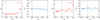 |
Fig. 5. PDF parameters as a function of the scale separation r. a) Trend of the parameter κ for the PSP data sample. The limit value of κ = 1.33 is highlighted by the horizontal line. b) Trend of the parameter λ for the PSP data sample. The value λ = 0 is indicated by the horizontal line. c) Trend of the parameter κ for the C3 data sample. The limit value of κ = 2.61 is highlighted by the horizontal line. d) Trend of the parameter λ for the C3 data sample. The value λ = 0 is indicated by the horizontal line. The vertical lines in all the panels mark the ion inertial length. |
Equation (23) provides a prediction for the PDF of magnetic field fluctuations at kinetic scales. The small-scale values assumed by κ in PSP and C3 data samples were used to draw this one-parameter distribution. A comparison to spacecraft observations is displayed in Figure 6. Starting from the smallest scales considered in the analysis (see Figure 3), we show the superposition of about one order of magnitude in scale separation, reaching scales of about di. The interval of the perpendicular fluctuation magnitude reported in the figure is ±10σr. The agreement between theoretical predictions and observation is remarkable especially for the interval within ±5σr. Because of the finite size of the samples, the heavy tails of the distributions are not well sampled, which results in slightly scattered points and/or cutoffs. However, from a physical point of view, a cutoff with respect to the ideal Kappa distribution must be observed as a consequence of the finite energy contained in the fluctuations, thus guaranteeing the finiteness of all high-order moments.
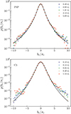 |
Fig. 6. Magnetic field fluctuation PDFs. The filled circles represent the statistics computed on PSP and C3 measurements at different scales and cover about one order of magnitude in the scale separation r. Theoretical predictions provided by the Kappa distribution are indicated by solid lines. |
The remarkable agreement between the model prediction and data reported in Figure 6 is a peculiar property of space-plasma kinetic fluctuations. At larger scales, the turbulent cascade generates an inhomogeneous energy transfer that is associated with the intermittency of fluctuations in a statistical sense. Intermittency is usually quantified by investigating the scale dependence of the flatness (Frisch 1995; Biskamp 2003). Changing values of the flatness can be associated with a scale-by-scale modification of the shape of the distribution function of the fluctuations, which means that it is impossible to obtain a master curve for the process by rescaling the stochastic variable with only one parameter (Sorriso-Valvo et al. 1999). Moreover, when we interpret the distribution (Eq. (23)) as an instantaneous stationary distribution at a fixed r, that is, by assuming the stationary solution of the FPE to be locally valid, the obtained stationary distributions do not capture the onset of the typical intermittent turbulent dynamics, with a tendency toward a dramatic underestimation of extreme fluctuations (Nickelsen & Engel 2013).
5. Discussion and conclusions
The multiscale approach developed by Friedrich & Peinke (1997) is effective in catching and reproducing the statistical properties of turbulent fluctuations that evolve across scales. This approach, previously extended to space plasma turbulence by Strumik & Macek (2008), was adapted to solar wind kinetic scales, where the statistics of magnetic field fluctuations is known to be globally self-similar (Kiyani et al. 2009; Osman et al. 2015). Therefore, starting from the hypothesis of self-similar scaling, we derived the master curve describing the distribution of magnetic field fluctuations, which is found to be a Kappa distribution. Efforts to link Kappa distributions observed in the statistics of the magnetic field fluctuations to the scale-to-scale stochastic process have recently been made by Benella et al. (2022a). Other authors later employed this framework to test the scale invariance of kinetic fluctuations observed in the magnetosheath and close to the magnetopause (Macek et al. 2023; Macek & Wójcik 2023; Wójcik & Macek 2024). The present work represents a step forward in this field, providing an analytical derivation of the master curve and linking the parameter κ of the Kappa distribution to the diffusion term D(br, r) associated with interplanetary magnetic field observations. The master curve derived in this work can be asymmetric with respect to zero, with the asymmetry controlled by the parameter λ, thus leading to a generalization of the standard Kappa distribution.
We excluded parallel fluctuations from statistics by selecting magnetic field increments within the 80° < θVB < 100° range. The reason for this is twofold. First, magnetic field fluctuations are strongly anisotropic and mostly develop in the perpendicular direction with respect to the local mean field, thus being representative of the global statistics. In this case, the master curve, obtained by introducing phenomenological arguments in the framework of stochastic processes, agrees with observations. The second reason is that parallel fluctuations encompass ion-resonant processes that might play a key role in mediating the collisionless dissipation of turbulent energy (Bowen et al. 2024). Whereas fluctuations associated with dominant circular polarized ion waves exhibit a global scale invariance, data samples with a weaker ion-resonant component may develop intermittency. The absence of circular ion waves is correlated with the occurrence of non-Gaussian intermittent fluctuations, which is indicative of small-scale current sheets. Hence, the hypothesis of stationary FPE, on which this work is based, may not always be satisfied for parallel fluctuations. From the physical side, the existence of a master curve can be related to the presence of homogeneous and globally self-similar fluctuations. The anomalous scaling observed in turbulence is associated with the inhomogeneity of the energy transfer. Therefore, the regularization of the scaling laws observed in the kinetic range and the emergence of a master curve suggest that energy transfer is homogenized at small scales. This scenario agrees with recent numerical results based on weak kinetic-Alfvén wave turbulence (David & Galtier 2019; David et al. 2024), but also with observations (Richard et al. 2024) of energy transfer/dissipation in near-Earth space plasmas.
The parameter κ of the master curve defined in Equation (22) measures the weight of q0(r) with respect to q2(r). In other words, κ represents the ratio of additive and multiplicative noise in the diffusion term (Eq. (13)) of the stochastic process br. The case of purely additive noise, that is, q2(r)→0, corresponds to the limit κ → ∞ where the master curve (Eq. (23)) tends toward a Gaussian density function. The heavy tails observed in the magnetic field statistics are thus associated with the multiplicative part of the stochastic dynamics, which plays a fundamental role in the stochastic modeling of kinetic-scale fluctuations. This finding helps us to advance this description, with the aim of assessing and understanding the meaning of the different terms appearing in the model. Benella et al. (2023) reported that the drift is the leading term in describing kinetic-scale fluctuations that are globally self-similar on average, thus being a proxy for a homogeneous energy transfer. In this case, the contribution of the diffusion term in determining average/global quantities, such as the scaling exponent, was neglected. We studied the probability density function instead of its moments, which allowed us to assess that the diffusion term plays a key role in defining the shape and asymmetry of the fluctuation PDF.
The derivation of κ and λ from the Langevin process provides a pair of parameters that are easily computed from spacecraft data that fully describe the statistics of kinetic-scale fluctuations. A systematic investigation of these parameters as a function of relevant quantities, such as radial distance from the Sun, Reynolds number, or the average magnitude of the magnetic field, is left as a future perspective, with the idea of relating it to a possible universal behavior of the fluctuations at these scales. Finally, we emphasize that the functional form of the drift and diffusion terms (empirical evidence) is based on the scaling arguments summarized in Section 2. The resulting stochastic process is associated with a master curve that resembles spacecraft in situ observations, thus providing interesting constraints on the phenomenology of small-scale dynamics. Future theoretical frameworks should include the statistical properties presented in this paper. The search for a phenomenology leading to Equations (7) and (8) thus represents the necessary and crucial step to take in future investigations.
Acknowledgments
Authors acknowledge Emiliya Yordanova for providing Cluster data and for the fruitful discussions. This work is supported by the mini-grant “The solar wind: a paradigm for complex system dynamics” financed by the National Institute for Astrophysics under the call “Fundamental Research 2022”. M.S acknowledges the mini-grant “Investigating the Universal Nature of Magnetic field Fluctuations in Solar Wind Turbulence: A Multifractal Approach” financed by the National Institute for Astrophysics under the call “Fundamental Research 2023”. PSP, Wind and SO data used in this study are available at the NASA Space Physics Data Facility (SPDF), https://spdf.gsfc.nasa.gov/index.html. The authors acknowledge the contributions of the FIELDS team to the Parker Solar Probe mission, the Cluster FGM, STAFF P.I.s and teams, and the ESA-Cluster Science Archive for making available the data used in this work.
References
- Alberti, T., Consolini, G., Carbone, V., et al. 2019, Entropy, 21, 320 [NASA ADS] [CrossRef] [Google Scholar]
- Arnèodo, A., Benzi, R., Berg, J., et al. 2008, Phys. Rev. Lett., 100, 254504 [CrossRef] [Google Scholar]
- Asensio Ramos, A., & Martínez González, M. J. 2014, A&A, 572, A98 [NASA ADS] [CrossRef] [EDP Sciences] [Google Scholar]
- Bale, S. D., Kellogg, P. J., Mozer, F. S., Horbury, T. S., & Reme, H. 2005, Phys. Rev. Lett., 94, 215002 [NASA ADS] [CrossRef] [Google Scholar]
- Bale, S. D., Goetz, K., Harvey, P. R., et al. 2016, Space Sci. Rev., 204, 49 [Google Scholar]
- Balogh, A., Dunlop, M. W., Cowley, S. W. H., et al. 1997, Space Sci. Rev., 79, 65 [CrossRef] [Google Scholar]
- Beck, C., & Cohen, E. G. D. 2003, Phys. A Stat. Mech. Appl., 322, 267 [NASA ADS] [CrossRef] [Google Scholar]
- Belcher, J. W., & Davis, L., Jr. 1971, J. Geophys. Res., 76, 3534 [NASA ADS] [CrossRef] [Google Scholar]
- Benella, S., Stumpo, M., Consolini, G., et al. 2022a, ApJ, 928, L21 [NASA ADS] [CrossRef] [Google Scholar]
- Benella, S., Stumpo, M., Consolini, G., et al. 2022b, Rendiconti Lincei. Scienze Fisiche e Naturali, 33, 721 [NASA ADS] [CrossRef] [Google Scholar]
- Benella, S., Stumpo, M., Alberti, T., et al. 2023, Phys. Rev. Res., 5, L042014 [NASA ADS] [CrossRef] [Google Scholar]
- Bian, N. H., & Li, G. 2022, ApJ, 941, 58 [NASA ADS] [CrossRef] [Google Scholar]
- Bian, N. H., & Li, G. 2024a, ApJ, 960, L15 [NASA ADS] [CrossRef] [Google Scholar]
- Bian, N. H., & Li, G. 2024b, ApJS, 273, 15 [NASA ADS] [CrossRef] [Google Scholar]
- Bian, N. H., Emslie, A. G., Stackhouse, D. J., & Kontar, E. P. 2014, ApJ, 796, 142 [NASA ADS] [CrossRef] [Google Scholar]
- Biskamp, D. 2003, Magnetohydrodynamic Turbulence (Cambridge: Cambridge University Press) [Google Scholar]
- Bowen, T. A., Bale, S. D., Bonnell, J. W., et al. 2020, J. Geophys. Res.: Space Phys., 125, e2020JA027813 [CrossRef] [Google Scholar]
- Bowen, T. A., Bale, S. D., Chandran, B. D. G., et al. 2024, Nat. Astron., 8, 482 [Google Scholar]
- Bruno, R., & Carbone, V. 2016, Turbulence in the Solar Wind, 928 [CrossRef] [Google Scholar]
- Carbone, V., Lepreti, F., Vecchio, A., Alberti, T., & Chiappetta, F. 2021, Front. Phys., 9, 18 [NASA ADS] [CrossRef] [Google Scholar]
- Carbone, V., Telloni, D., Lepreti, F., & Vecchio, A. 2022, ApJ, 924, L26 [NASA ADS] [CrossRef] [Google Scholar]
- Castaing, B., & Dubrulle, B. 1995, J. Phys. II, 5, 895 [NASA ADS] [Google Scholar]
- Chasapis, A., Matthaeus, W. H., Parashar, T. N., et al. 2017, ApJ, 844, L9 [NASA ADS] [CrossRef] [Google Scholar]
- Chen, C. H. K., Boldyrev, S., Xia, Q., & Perez, J. C. 2013, Phys. Rev. Lett., 110, 225002 [Google Scholar]
- Chhiber, R., Matthaeus, W. H., Bowen, T. A., & Bale, S. D. 2021, ApJ, 911, L7 [NASA ADS] [CrossRef] [Google Scholar]
- Chiappetta, F., Yordanova, E., Vörös, Z., Lepreti, F., & Carbone, V. 2023, ApJ, 957, 98 [NASA ADS] [CrossRef] [Google Scholar]
- Coleman, P. J., Jr. 1968, ApJ, 153, 371 [NASA ADS] [CrossRef] [Google Scholar]
- Collier, M. R., Hamilton, D. C., Gloeckler, G., Bochsler, P., & Sheldon, R. B. 1996, Geophys. Res. Lett., 23, 1191 [NASA ADS] [CrossRef] [Google Scholar]
- Consolini, G., Kretzschmar, M., Lui, A. T. Y., Zimbardo, G., & Macek, W. M. 2005, J. Geophys. Res. (Space Phys.), 110, A07202 [CrossRef] [Google Scholar]
- Cornilleau-Wehrlin, N., Chauveau, P., Louis, S., et al. 1997, Space Sci. Rev., 79, 107 [CrossRef] [Google Scholar]
- Cranmer, S. R., & van Ballegooijen, A. A. 2003, ApJ, 594, 573 [NASA ADS] [CrossRef] [Google Scholar]
- David, V., & Galtier, S. 2019, ApJ, 880, L10 [NASA ADS] [CrossRef] [Google Scholar]
- David, V., Galtier, S., & Meyrand, R. 2024, Phys. Rev. Lett., 132, 085201 [NASA ADS] [CrossRef] [Google Scholar]
- Dubrulle, B. 1994, Phys. Rev. Lett., 73, 959 [NASA ADS] [CrossRef] [Google Scholar]
- Fisk, L. A., & Gloeckler, G. 2014, J. Geophys. Res. (Space Phys.), 119, 8733 [CrossRef] [Google Scholar]
- Friedrich, J., & Grauer, R. 2020, Atmosphere, 11, 1003 [NASA ADS] [CrossRef] [Google Scholar]
- Friedrich, R., & Peinke, J. 1997, Phys. Rev. Lett., 78, 863 [NASA ADS] [CrossRef] [Google Scholar]
- Frisch, U. 1995, Turbulence. The legacy of A.N. Kolmogorov (Cambridge: Cambridge University Press) [CrossRef] [Google Scholar]
- Fuchs, A., Herbert, C., Rolland, J., et al. 2022, Phys. Rev. Lett., 129, 034502 [NASA ADS] [CrossRef] [Google Scholar]
- Gorobets, A. Y., Borrero, J. M., & Berdyugina, S. 2016, ApJ, 825, L18 [NASA ADS] [CrossRef] [Google Scholar]
- Gravanis, E., Akylas, E., Panagiotou, C., & Livadiotis, G. 2019, Entropy, 21, 1093 [NASA ADS] [CrossRef] [Google Scholar]
- Gravanis, E., Akylas, E., & Livadiotis, G. 2020, EPL, 130, 30005 [NASA ADS] [CrossRef] [EDP Sciences] [Google Scholar]
- Higdon, J. C. 1984, ApJ, 285, 109 [Google Scholar]
- Horbury, T. S., Forman, M., & Oughton, S. 2008, Phys. Rev. Lett., 101, 175005 [Google Scholar]
- Horbury, T. S., Wicks, R. T., & Chen, C. H. K. 2012, Space Sci. Rev., 172, 325 [Google Scholar]
- Kiyani, K., Chapman, S., Khotyaintsev, Y. V., Dunlop, M., & Sahraoui, F. 2009, Phys. Rev. Lett., 103, 075006 [NASA ADS] [CrossRef] [Google Scholar]
- Kolmogorov, A. 1941, Akademiia Nauk SSSR Doklady, 30, 301 [Google Scholar]
- Kolmogorov, A. N. 1962, J. Fluid Mech., 13, 82 [Google Scholar]
- Kraichnan, R. H. 1965, Phys. Fluids, 8, 1385 [Google Scholar]
- Lazar, M., & Fichtner, H. 2021, Astrophys. Space Sci. Lib., 464 [CrossRef] [Google Scholar]
- Leonardis, E., Sorriso-Valvo, L., Valentini, F., et al. 2016, Phys. Plasmas, 23, 022307 [CrossRef] [Google Scholar]
- Leubner, M. P., & Vörös, Z. 2005, ApJ, 618, 547 [NASA ADS] [CrossRef] [Google Scholar]
- Livadiotis, G. 2017, Kappa Distributions: Theory and Applications in Plasmas (Elsevier) [Google Scholar]
- Livadiotis, G. 2019, ApJ, 886, 3 [NASA ADS] [CrossRef] [Google Scholar]
- Livadiotis, G., & McComas, D. J. 2010, Phys. Scr., 82, 035003 [CrossRef] [Google Scholar]
- Livadiotis, G., McComas, D. J., Randol, B. M., et al. 2012, ApJ, 751, 64 [NASA ADS] [CrossRef] [Google Scholar]
- Livadiotis, G., McComas, D. J., & Shrestha, B. L. 2024, ApJ, 968, 66 [NASA ADS] [CrossRef] [Google Scholar]
- L’Vov, V. S. 1998, Nature, 396, 519 [CrossRef] [Google Scholar]
- Macek, W. M., & Wójcik, D. 2023, MNRAS, 526, 5779 [CrossRef] [Google Scholar]
- Macek, W. M., Wójcik, D., & Burch, J. L. 2023, ApJ, 943, 152 [NASA ADS] [CrossRef] [Google Scholar]
- Maksimovic, M., Pierrard, V., & Lemaire, J. F. 1997, A&A, 324, 725 [NASA ADS] [Google Scholar]
- Mann, G., Classen, H. T., Keppler, E., & Roelof, E. C. 2002, A&A, 391, 749 [NASA ADS] [CrossRef] [EDP Sciences] [Google Scholar]
- Marsch, E. 2006, Liv. Rev. Sol. Phys., 3, 1 [Google Scholar]
- Nickelsen, D. 2017, J. Stat. Mech: Theory Exp., 7, 073209 [NASA ADS] [CrossRef] [Google Scholar]
- Nickelsen, D., & Engel, A. 2013, Phys. Rev. Lett., 110, 214501 [NASA ADS] [CrossRef] [Google Scholar]
- Obukhov, A. M. 1962, J. Geophys. Res., 67, 3011 [NASA ADS] [CrossRef] [Google Scholar]
- Olbert, S. 1968, Astrophys. Space Sci. Lib., 10, 641 [NASA ADS] [CrossRef] [Google Scholar]
- Osman, K. T., Kiyani, K. H., Matthaeus, W. H., et al. 2015, ApJ, 815, L24 [NASA ADS] [CrossRef] [Google Scholar]
- Parisi, G., & Frisch, U. 1985, in Fully Developed Turbulence and Intermittency, eds. M. Ghil, R. Benzi, & G. Parisi, (New York: North-Holland), 84 [Google Scholar]
- Pavlos, G. P., Malandraki, O. E., Pavlos, E. G., Iliopoulos, A. C., & Karakatsanis, L. P. 2016, Phys. A Stat. Mech. Appl., 464, 149 [NASA ADS] [CrossRef] [Google Scholar]
- Pierrard, V., Maksimovic, M., & Lemaire, J. 1999, J. Geophys. Res., 104, 17021P [NASA ADS] [CrossRef] [Google Scholar]
- Podesta, J. J. 2009, ApJ, 698, 986 [NASA ADS] [CrossRef] [Google Scholar]
- Podesta, J. J., & Gary, S. P. 2011, ApJ, 734, 15 [NASA ADS] [CrossRef] [Google Scholar]
- Reinke, N., Fuchs, A., Nickelsen, D., & Peinke, J. 2018, J. Fluid Mech., 848, 117 [NASA ADS] [CrossRef] [Google Scholar]
- Renner, C., Peinke, J., & Friedrich, R. 2001, J. Fluid Mech., 433, 383 [NASA ADS] [CrossRef] [Google Scholar]
- Richard, L., Sorriso-Valvo, L., Yordanova, E., Graham, D. B., & Khotyaintsev, Y. V. 2024, Phys. Rev. Lett., 132, 105201 [NASA ADS] [CrossRef] [Google Scholar]
- Risken, H. 1996, Fokker-Planck Equation (Springer), 63 [CrossRef] [Google Scholar]
- Sahraoui, F., & Huang, S. 2023, ApJ, 956, 89 [NASA ADS] [CrossRef] [Google Scholar]
- Sahraoui, F., Huang, S. Y., Belmont, G., et al. 2013, ApJ, 777, 15 [NASA ADS] [CrossRef] [Google Scholar]
- Schwadron, N. A., Dayeh, M. A., Desai, M., et al. 2010, ApJ, 713, 1386 [Google Scholar]
- She, Z.-S., & Leveque, E. 1994, Phys. Rev. Lett., 72, 336 [Google Scholar]
- Sorriso-Valvo, L., Carbone, V., Veltri, P., Consolini, G., & Bruno, R. 1999, J. Geophys. Res., 26, 1801 [NASA ADS] [Google Scholar]
- Strumik, M., & Macek, W. M. 2008, Phys. Rev. E, 78, 026414 [NASA ADS] [CrossRef] [Google Scholar]
- Tabar, M. R. R. 2019, Analysis and Data-based Reconstruction of Complex Nonlinear Dynamical Systems (Springer), 730 [CrossRef] [Google Scholar]
- Vasyliunas, V. M. 1968, J. Geophys. Res., 73, 2839 [NASA ADS] [CrossRef] [Google Scholar]
- Wójcik, D., & Macek, W. M. 2024, Phys. Rev. E, 110, 025203 [CrossRef] [Google Scholar]
- Yakhot, V. 1998, Phys. Rev. E, 57, 1737 [NASA ADS] [CrossRef] [Google Scholar]
- Yoon, P. H. 2012, Phys. Plasmas, 19, 052301 [NASA ADS] [CrossRef] [Google Scholar]
- Yoon, P. H. 2014, J. Geophys. Res. (Space Phys.), 119, 7074 [CrossRef] [Google Scholar]
- Yoon, P. H. 2020, Eur. Phys. J. Special Top., 229, 819 [NASA ADS] [CrossRef] [Google Scholar]
- Yordanova, E., Perri, S., Sorriso-Valvo, L., & Carbone, V. 2015, EPL, 110, 19001 [NASA ADS] [CrossRef] [EDP Sciences] [Google Scholar]
- Zank, G. P., Li, G., Florinski, V., et al. 2006, J. Geophys. Res. (Space Phys.), 111, A06108 [CrossRef] [Google Scholar]
- Zhuravleva, I., Churazov, E., Schekochihin, A. A., et al. 2014, Nature, 515, 85 [Google Scholar]
- Zouganelis, I. 2008, J. Geophys. Res. (Space Phys.), 113, A08111 [CrossRef] [Google Scholar]
Appendix A: Derivation of the master curve
For general purposes and a more clear connection with the literature, we will use here t ≥ 0 as independent “time” variable for the Fokker-Planck description of a real Itô stochastic process (Xt)t ≥ 0 satisfying

with (Wt)t ≥ 0 being a standard Wiener process. All the formulas in the remaining text can be obtained via some suitable change of variable, such as r = r0e−t/τ, or r = r0 − Vt, together with a redefinition of the drift M and the diffusion coefficient D. Notice that r decreases while t increases.
The probability density ρt(X) of finding Xt in the state X is defined by the relation
for any subset I ⊆ ℝ and it has a unitary integral over the definition domain
Assuming the initial density function ρ0(X) to be known, the generalized Langevin equation (A.1) is equivalent to the FPE (Risken 1996)
![$$ \begin{aligned} \frac{\partial \rho _r(X)}{\partial t} = \frac{\partial }{\partial X}\biggl [\frac{\partial }{\partial X}(D(X,t)\rho _t(X)) - M(X,t)\rho _t(X)\biggr ]. \end{aligned} $$](/articles/aa/full_html/2024/10/aa50714-24/aa50714-24-eq31.gif)
The derivation of Equation (A.3) with respect to t gives the following condition on the boundary terms:
![$$ \begin{aligned} \biggl [\frac{\partial }{\partial X}(D(X,t)\rho _t(X)) - M(X,t)\rho _t(X)\biggr ]^{+\infty }_{-\infty } = 0. \end{aligned} $$](/articles/aa/full_html/2024/10/aa50714-24/aa50714-24-eq32.gif)
We define the mean and the variance of Xt as
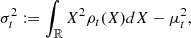
respectively, and we assume that both are finite. By deriving μt and σt2 with respect to t, we obtain
![$$ \begin{aligned} \frac{d\mu _t}{dt} = \int _{\mathbb{R} } M(X,t)\rho _t(X)dX - \biggl [D(X,t)\rho _t(X)\biggr ]^{+\infty }_{-\infty } \end{aligned} $$](/articles/aa/full_html/2024/10/aa50714-24/aa50714-24-eq35.gif)
and
![$$ \begin{aligned} \frac{d\sigma ^2_t}{dt}&= 2\int _{\mathbb{R} } (D(X,t) + XM(X,t))\rho _t(X)dX - 2\mu _t\frac{d\mu _t}{dt}\nonumber \\&\quad - 2\biggl [XD(X,t)\rho _t(X)\biggr ]^{+\infty }_{-\infty }, \end{aligned} $$](/articles/aa/full_html/2024/10/aa50714-24/aa50714-24-eq36.gif)
where Equation (A.5) has been used. Assuming the polynomial drift and diffusion terms introduced in Equations (7) and (8) and assuming vanishing boundary terms in Equations (A.8, A.9), we get the following closed system of differential equations
![$$ \begin{aligned} \frac{d\sigma ^2_t}{dt} = 2[L_1(t) + Q_2(t)]\sigma ^2_t + 2Q(\mu _t,t), \end{aligned} $$](/articles/aa/full_html/2024/10/aa50714-24/aa50714-24-eq38.gif)
whose solutions are
and
![$$ \begin{aligned} \sigma ^2_t&= \sigma ^2_0\exp \biggl (2\int _0^t[L_1(u) + Q_2(u)]du\biggr )\nonumber \\&+ 2\int _0^tQ(\mu _s,s)\exp \biggl (2\int _s^t[L_1(u) + Q_2(u)]du\biggr )ds. \end{aligned} $$](/articles/aa/full_html/2024/10/aa50714-24/aa50714-24-eq40.gif)
By introducing the standardized process (xt)t ≥ 0
the probability density pt(x) of finding xt at x is given by

It satisfies the following FPE
![$$ \begin{aligned} \frac{\partial p_t(x)}{\partial t} = \frac{\partial }{\partial x}\biggl [ \frac{\partial }{\partial x}(d(x,t)p_t(x)) - m(x,t)p_t(x)\biggr ], \end{aligned} $$](/articles/aa/full_html/2024/10/aa50714-24/aa50714-24-eq43.gif)
with drift and diffusion coefficients given by
In the special case of M ≡ L and D ≡ Q, e.g., see Equations (7) and (8), we get m ≡ l and d ≡ q, where
![$$ \begin{aligned}&l(x,t) := - [q_0(t) + q_2(t)]x \end{aligned} $$](/articles/aa/full_html/2024/10/aa50714-24/aa50714-24-eq46.gif)

where the terms q0, q1 and q2 are
If the process (xt)t ≥ 0 is stationary, viz., ∂pt/∂t ≡ 0, we can write pt(x)≡p(x) and hence
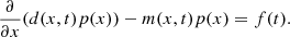
Furthermore, f(t) must vanish identically, as a consequence of (A.8). The solution can then be written as
![$$ \begin{aligned} p(x) = p(\bar{x})\exp \biggl [\int _{\bar{x}}^x\frac{m(y,t) - \partial d(y,t)/\partial y}{d(y,t)} dy\biggr ], \end{aligned} $$](/articles/aa/full_html/2024/10/aa50714-24/aa50714-24-eq52.gif)
with some arbitrary  , which can be suitably chosen. The probability density p is called a master curve.
The explicit dependence on t in (A.25) must be completely reabsorbed, for the probability density to be stationary, thus we obtain the condition
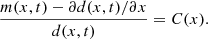
In the special case when m ≡ l and d ≡ q, we get C ≡ Cκ, λ, with
![$$ \begin{aligned} C_{\kappa ,\lambda }(x) := \frac{2[\lambda - (\kappa +1)x]}{2\kappa - 1 - 2\lambda x + x^2}, \end{aligned} $$](/articles/aa/full_html/2024/10/aa50714-24/aa50714-24-eq55.gif)
where 2κ − 1 > λ2, leading to

In this case, by choosing  , the corresponding stationary probability density follows to be

where
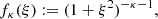
with i being the imaginary unit and Γ the Euler gamma function:
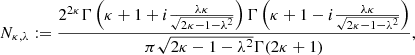
To get the normalization constant Nκ, λ we made use of the following identity

together with
which has been found as a condition for the integral (A.34) to be real, where the incomplete beta function is defined as
Appendix B: Finite-scale estimation of KM coefficients
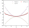 |
Fig. B.1. Example of finite scale KM coefficient estimation. Filled circles represent non parametrical estimation of DΔ(b, r), purple, ϵΔ(b, r), beige, and σr2 DΔ(x, r), red. Solid lines indicate the second-order polynomial fits. |
An interesting feature in the derivation of the drift-diffusion parameters for the standardized variable x is their dependence upon the diffusion coefficient D of the magnetic field fluctuations only. All the relations derived in Section 3 are based on the calculation of the KM coefficients, which are the limit of the conditional moments (Risken 1996). Hence, the second-order KM coefficient (viz., diffusion term) can be written as
![$$ \begin{aligned} D(b,r)=\lim _{\Delta \rightarrow 0}\frac{1}{2!\Delta }\mathbb{E} [(b(r-\Delta )-b(r))^2|b(r)]. \end{aligned} $$](/articles/aa/full_html/2024/10/aa50714-24/aa50714-24-eq66.gif)
The limit of vanishing separation Δ is a daunting task when dealing with "real-world" timeseries. In this work we set the separation Δ to be finite and small, close to the resolution of the data, but large enough to avoid effect due to the instrumental noise at high frequencies. When the values of Δ is finite, although arbitrary small, we need to consider the correction terms appearing in the change from the variable b to the standardized variable x = b/σr. In the ideal case of vanishing Δ we used the relation
According to Benella et al. (2022b), in the case of finite and arbitrary small Δ, we must introduce the following correction

with ϵΔ(br, r) defined as (Benella et al. 2022b)
![$$ \begin{aligned} \epsilon _\Delta (b_r,r)&= \frac{1}{2\Delta }\biggl (\frac{\sigma _r^2}{\sigma _r^{\prime 2}}-1\biggr )\,\mathbb{E} [b^2(r-\Delta )|b(r)]\nonumber \\&+\frac{1}{\Delta }\biggl (1-\frac{\sigma _r}{\sigma _r^{\prime }}\biggr )\,\mathbb{E} [b(r-\Delta )b(r)|b(r)]. \end{aligned} $$](/articles/aa/full_html/2024/10/aa50714-24/aa50714-24-eq69.gif)
The correction term ϵΔ(br, r) exhibits a quadratic trend as the diffusion term DΔ(br, r), thus we can introduce a quadratic parametrization also for ϵΔ(br, r). An graphical example of the transformation between DΔ(b, r) and DΔ(x, r) calculated on C3 data at the fixed scale r = 0.1 di is shown in Figure B.1. Circles indicate DΔ(b, r = 0.1 di) in purple, the correction ϵΔ(b, r = 0.1 di) in beige, and the diffusion term of the standardized variable σr2 DΔ(x, r = 0.1 di) in red, while solid lines show their second-order polynomial fits.
All Tables
All Figures
|
Fig. 1. Example of a stationary distribution (Eq. (19)) with κ = 1 for different values of λ. The dashed line indicates λ = −0.2, the dotted line shows λ = 0.2, and the solid line shows the Kappa distribution (Eq. (23)). |
| In the text | |
|
Fig. 2. Radial component of the magnetic field BR observed by PSP during the first perihelion (left), and magnetic field component Bx in the GSE coordinate system observed by the C3 spacecraft (right). |
| In the text | |
|
Fig. 3. Power spectral density of the 2018 November 9 PSP data interval (left) and of the 2007 January 20 C3 data sample (right). Vertical lines indicate frequencies associated with the ion inertial length (red) and the ion gyroradius (green). The blue lines indicate the smallest scales considered in the analysis. The typical slopes in the inertial and kinetic ranges are reported for reference (dotted lines). |
| In the text | |
|
Fig. 4. Histograms of the angle θVB between the local mean magnetic field and the sampling direction for the PSP and C3 data samples. The statistics have been calculated at scale τ = 0.03 s, and the vertical lines delineate the region 80° < θVB < 100° around the perpendicular direction. |
| In the text | |
|
Fig. 5. PDF parameters as a function of the scale separation r. a) Trend of the parameter κ for the PSP data sample. The limit value of κ = 1.33 is highlighted by the horizontal line. b) Trend of the parameter λ for the PSP data sample. The value λ = 0 is indicated by the horizontal line. c) Trend of the parameter κ for the C3 data sample. The limit value of κ = 2.61 is highlighted by the horizontal line. d) Trend of the parameter λ for the C3 data sample. The value λ = 0 is indicated by the horizontal line. The vertical lines in all the panels mark the ion inertial length. |
| In the text | |
|
Fig. 6. Magnetic field fluctuation PDFs. The filled circles represent the statistics computed on PSP and C3 measurements at different scales and cover about one order of magnitude in the scale separation r. Theoretical predictions provided by the Kappa distribution are indicated by solid lines. |
| In the text | |
|
Fig. B.1. Example of finite scale KM coefficient estimation. Filled circles represent non parametrical estimation of DΔ(b, r), purple, ϵΔ(b, r), beige, and σr2 DΔ(x, r), red. Solid lines indicate the second-order polynomial fits. |
| In the text | |
Current usage metrics show cumulative count of Article Views (full-text article views including HTML views, PDF and ePub downloads, according to the available data) and Abstracts Views on Vision4Press platform.
Data correspond to usage on the plateform after 2015. The current usage metrics is available 48-96 hours after online publication and is updated daily on week days.
Initial download of the metrics may take a while.