| Issue |
A&A
Volume 690, October 2024
|
|
|---|---|---|
| Article Number | A353 | |
| Number of page(s) | 9 | |
| Section | Astrophysical processes | |
| DOI | https://doi.org/10.1051/0004-6361/202450581 | |
| Published online | 22 October 2024 | |
Discovery of SRGA J144459.2−604207 with the SRG/ART-XC telescope: A well-tempered bursting accreting millisecond X-ray pulsar
1
Space Research Institute, Russian Academy of Sciences, Profsoyuznaya 84/32, 117997 Moscow, Russia
2
Department of Physics and Astronomy, FI-20014 University of Turku, Turku, Finland
3
Institut für Astronomie und Astrophysik, Universität Tübingen, Sand 1, D-72076 Tübingen, Germany
Received:
1
May
2024
Accepted:
6
September
2024
We report the discovery of the new accreting millisecond X-ray pulsar SRGA J144459.2−604207 using data of the SRG/ART-XC. The source was observed twice in February 2024 during the declining phase of the outburst. The timing analysis revealed a coherent signal near 447.9 Hz modulated by the Doppler effect due to the orbital motion. The derived parameters for the binary system are consistent with a circular orbit with a period of ∼5.2 h. The pulse profiles of the persistent emission, showing a sine-like part during half a period with a plateau in between, can be well modeled by emission from two circular spots that are partially eclipsed by the accretion disk. Additionally, during our observations with an exposure of 133 ks, we detected 19 thermonuclear X-ray bursts. All bursts have similar shapes and energetics, and none show any signs of an expanding photospheric radius. The burst recurrence times decreases linearly from ∼1.6 h at the beginning of observations to ∼2.2 h at the end and anticorrelate with the persistent flux. The spectral evolution during the bursts is consistent with the models of the neutron star atmospheres that are heated by accretion and implies a neutron star radius of 11–12 km and a distance to the source of 8–9 kpc. We also detected coherent pulsations during the bursts and showed that the pulse profiles differ substantially from those observed in the persistent emission. However, we could not find a simple physical model explaining the pulse profiles detected during the bursts.
Key words: binaries: general / stars: neutron / stars: oscillations / pulsars: individual: SRGA J144459.2–604207
© The Authors 2024
 Open Access article, published by EDP Sciences, under the terms of the Creative Commons Attribution License (https://creativecommons.org/licenses/by/4.0), which permits unrestricted use, distribution, and reproduction in any medium, provided the original work is properly cited.
This article is published in open access under the Subscribe to Open model. Subscribe to A&A to support open access publication.
1. Introduction
Accreting millisecond X-ray pulsars (AMXPs) constitute a relatively small group of binary systems featuring a rapidly rotating neutron star (NS) and a low-mass optical companion (see Patruno & Watts 2021; Di Salvo & Sanna 2022, for recent reviews). The NSs in these systems, which are thought to be progenitors of rotation-powered millisecond pulsars, exhibit spin periods ranging from ∼1.7 to ∼10 ms and possess relatively weak magnetic fields (around 108–109 G). Thus, these objects play an important role in the stellar evolutionary processes, but the current sample of known AMXPs comprises only about two dozen sources. Therefore, a search for these objects and their discoveries is a quite important task. Moreover, this task is highly nontrivial and demands extraordinary technical capabilities of X-ray instruments, including a large effective area and a high time resolution.
The Mikhail Pavlinsky ART-XC telescope (Pavlinsky et al. 2021) on board the Spectrum-Roentgen-Gamma observatory (SRG; Sunyaev et al. 2021) discovered a new AMXP, SRGA J144459.2−604207 (hereafter SRGA J1444) during the ongoing all-sky survey. The source was found on 2024 February 21 at a position close to the Galactic plane with coordinates (l, b) ≃ ( ) and a flux of ∼100 mCrab in the 4–12 keV energy band (Mereminskiy et al. 2024).
The intense follow-up campaign carried out immediately after the discovery revealed that SRGA J1444 is a new accreting millisecond pulsar with a spin period of 447.9 Hz (Ng et al. 2024a) showing regular type I X-ray bursts (Mariani et al. 2024; Ray et al. 2024; Sanchez-Fernandez et al. 2024). Subsequent observations of SRGA J1444 with the Neutron star Interior Composition Explorer (NICER) and the Hard X-ray Modulation Telescope (Insight-HXMT) unveiled a clear sinusoidal Doppler shift of the spin frequency that allowed us to determine an orbital period of ∼5.2 h, indicating that the companion star mass exceeds 0.255 M⊙ (Ray et al. 2024; Li et al. 2024).
The improved coordinates of SRGA J1444, RA (J2000) = , Dec (J2000)
  , were obtained with the High Resolution Camera on board the Chandra observatory (Illiano et al. 2024). Despite the accurate localization of the source, no optical or IR counterpart was found (Sokolovsky et al. 2024; Cowie et al. 2024; Baglio et al. 2024; Saikia et al. 2024). A radio counterpart was discovered at the position of SRGA J1444 using the Australia Telescope Compact Array (Russell et al. 2024). Its spectral index is consistent with the emission from either a compact jet or discrete ejecta from an X-ray binary. It is interesting that the retrospective analysis of the Monitor of All-sky X-ray Image (MAXI) and the International Gamma-Ray Astrophysics Laboratory (INTEGRAL) archival data revealed past X-ray activity of SRGA J1444. Particularly, an increase in the flux from the sky position coincident with that of the SRGA J1444 was observed in the beginning of January 2022 and mid-December 2023 (Negoro et al. 2024; Sguera & Sidoli 2024).
In this paper, we report the discovery of a new AMXP SRGA J1444 using the ART-XC telescope data. The results of the timing and spectral analysis of both the persistent emission and its evolution during multiple type I bursts are presented, as is the modeling of the bursts and the pulse profile.
2. Observations and data reduction
SRGA J1444 was first detected in the data downlinked from the ART-XC telescope on 2024 February 21 using a near-real-time data-processing chain. It was quickly identified as a new X-ray source located in the Galactic plane. At the time of detection, the source flux was about (1.9 ± 0.1)×10−9 erg cm−2 s−1 in the 4–12 keV band (Mereminskiy et al. 2024, see also Fig. 1). Two extended observations were conducted with the ART-XC telescope as part of the follow-up program. The first observation began on 2024 February 24 and lasted for 28 ks, while the second observation started on 2024 February 26 and continued for 105 ks.
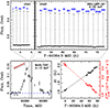 |
Fig. 1. Temporal evolution of the SRGA J1444 emission during the 2024 outburst. Upper panel: ART-XC light curve during two observations. The time and mean flux of the type I X-ray bursts are shown with the dashed line and thick streak. Bottom left: Flux evolution as observed by MAXI/GSC in the 4–10 keV energy band. Bottom right: X-ray burst recurrence time (in black, left axis) and the mean persistent flux between the bursts in the 4–25 keV energy band |

The ART-XC telescope is an imaging instrument consisting of seven modules and operating in the photon-counting mode (Pavlinsky et al. 2021) in the 4–30 keV energy band. The time resolution of the instrument is ∼23 μs. The data were processed using the ARTPRODUCTS v1.0 software with the latest CALDB V20220908. For the spectral and timing analysis, we extracted photons from a circle with a radius of 1 8 around the source position, and we also applied an energy filtering when needed. The background was estimated by collecting photons from a circular region with a radius of 3
 6 on the detectors that did not overlap with the region in which the source photons were extracted. Due to the limited energy band of ART-XC, which does not permit a reliable determination of a moderate interstellar absorption, we employed models with the fixed equivalent hydrogen column density of 2.7 × 1022 cm−2 to fit the energy spectra. This column density was determined from the NICER data (Ng et al. 2024a). All reported flux values in the paper are unabsorbed unless explicitly stated otherwise.
3. Persistent emission and bursting behavior
Observations of SRGA J1444 with the ART-XC telescope were carried out soon after the maximum of the outburst in the declining phase (Fig. 1, lower left panel). In total, a total of 19 type I X-ray bursts were registered in two observations, each lasting about 45 s and occurring at approximately equal intervals of about two hours. However, a detailed study showed that the recurrence time Δt between the bursts is not constant. It increases linearly from ∼1.6 h at the beginning of observations to ∼2.2 h at the end (Fig. 1, lower right panel), while the energy release during the bursts remains approximately at the same level (Fig. 1, upper panel).
To trace the evolution of the persistent emission, we split our observations into intervals of about 800 s and excluded X-ray bursts from the analysis. Then, we determined the average count rate in the 4–25 keV energy band for each interval. The resulting light curve in Crab flux units is presented in the upper panel of Fig. 1. The X-ray flux between consecutive bursts varies within 5%.
To quantify the rate of change in the persistent flux and to establish its relation with the burst generation frequency, we first reconstructed the energy spectra during intervals between the bursts. Then, we fit these spectra with a simple analytical model consisting of the absorbed power law with a high-energy cutoff, tbabs × cutoffpl in XSPEC (Arnaud 1996), and estimated the corresponding fluxes. All spectra have a similar shape and are well approximated by this model with a photon index of Γ ∼ 1.8 and a high-energy cutoff Ecut ∼ 25 keV, and they only differ in their normalizations. As an example, one of the spectra of the persistent emission extracted between bursts II and III is shown in Fig. 2. The evolution of the flux between the bursts is presented in the lower right panel in Fig. 1 (in red). It clearly shows that this flux is anticorrelated with the recurrence time of the bursts. At the same time, the total energy released between the bursts in the 4–25 keV energy band remains approximately constant, with the fluence being Ebet_brst ≃ 1.48 × 10⁻⁵ erg cm−2.
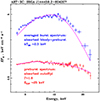 |
Fig. 2. Average energy spectrum of all type I X-ray bursts observed by ART-XC during the first observation (blue crosses) and the spectrum of the persistent emission extracted between bursts II and III (red crosses). The pink curves represent the spectral model of the absorbed blackbody and the cutoff power law. |
3.1. Type I X-ray bursts
First of all, the averaged energy spectrum for each of the bursts was analyzed. We reconstructed ART-XC spectra in the 4–25 keV energy band that were collected during 45 s time intervals starting from the beginning of the burst. The total spectrum of the source during the burst consists of the persistent emission and of the spectrum of a thermonuclear flash itself. The contribution of the persistent emission to the total burst spectrum was estimated by constructing the energy spectrum of the source during the 800 s preceding the burst. All pre-burst spectra are well approximated by the cutoff power-law model and the same parameters within the uncertainties as for the persistent emission (see Sect. 3). In order to describe the energy spectra of thermonuclear bursts, we approximated them with the two-component model, including a blackbody and a cutoff power law (modified by interstellar absorption with a fixed equivalent hydrogen column density; see above). The parameters of the second component, excluding normalization, were fixed at the values obtained for the persistent emission.
This model describes all 19 bursts relatively well with the same blackbody flux of F4 − 25 ≃ 8 × 10⁻⁹ erg cm−2 s−1 and the temperature, kTbb ≃ 2.3 keV, within the error bars (see Fig. 2). The fluence released per burst in the 4–25 keV energy band is about 3.6 × 10⁻⁷ erg cm−2.
We also investigated the morphology of the bursts and found that all the bursts have a similar shape, with a fast rise that transforms into a plateau-like phase, which in turn changes to exponential decay (see the upper part of Fig. 3). The similarity of the burst profiles and their spectral parameters gives us the opportunity to analyze not each burst individually, but their sum, which significantly improves the statistical errors and allows us to study emission properties with a better time resolution. In the lower panel of Fig. 3, we present an average burst profile with a time resolution of 1 s. Below, we study the spectral evolution during the bursts in more detail.
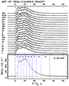 |
Fig. 3. Light curves of all detected type I X-ray bursts in the 4–25 keV energy band. The bottom panel shows the averaged burst profile. The dashed vertical lines represent the time intervals we used for the time-resolved spectral analysis (see Sect. 3.2). |
3.2. Time-resolved spectral analysis of the bursts
In order to investigate the spectral evolution of the radiation during X-ray bursts, we divided the averaged burst profile into nine time intervals (see the bottom panel of Fig. 3) and reconstructed energy spectra for them. The contribution of the persistent emission was taken into account in the same way as described above, that is, using it as background for approximating the bursts spectra. To describe these spectra, we used the blackbody model (modified by the fixed interstellar absorption), which adequately describes the spectra for all time intervals. The evolution of the blackbody parameters during the bursts is shown in Fig. 4. The blackbody normalization Kbb was converted into the radius of the emission region for the distance of 10 kpc:  . In the lower part of the figure, we also show the flux evolution in the energy range of 4–25 keV. There are no signatures of a photospheric radius expansion during the bursts. The burst peak bolometric luminosity Lpk ≃ 3.2 × 1038 erg s−1 (obtained from the peak flux of F4 − 25 ≃ 2.4 × 10⁻⁸ erg cm−2 s−1) is reached in about ten seconds, and the total energy release during the burst is approximately Ebst ≃ 5.1 × 1039 erg (again, a distance of 10 kpc is assumed).
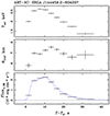 |
Fig. 4. Time-resolved spectroscopy of the averaged X-ray burst emission. The dotted blue line in the bottom panel shows the rescaled in amplitude count-rate light curve in 4–25 keV to match the measured fluxes. The pre-burst rate is subtracted. |
4. Timing properties
In this section, we investigate the timing properties of SRGA J1444, including pulsations, orbital motion, and the evolution of the pulse profile with time and energy both for the persistent emission and during the type I X-ray bursts.
4.1. Orbital parameters and coherent timing
A coherent signal near 447.8 Hz from SRGA J1444 was discovered by NICER (Ng et al. 2024a), and the later parameters of the binary motion were preliminarily determined based on the long set of NICER observations (Ray et al. 2024). Pulsations along with the sinusoidal modulation of its frequency with time are also clearly detected in the ART-XC data. To determine the spin period and orbital parameters, our observations were divided into segments of approximately 800 s for the subsequent analysis (type I X-ray bursts were excluded). Power spectra were then computed for each data segment to measure the frequency associated with this spin period. The resulting spin-frequency evolution is presented in Fig. 5. Furthermore, assuming a circular motion, we obtain the following orbital parameters for the binary system: an orbital period of Porb = 0.217649(5) d, a projected semi-major axis ax sin i = 0.6513(2) lt-s, a time of passage through the ascending node Tasc= MJD 60 361.64126(5), and a spin frequency ν = 447.8718(2) Hz. These values agree well with the parameters obtained from NICER (Ray et al. 2024) and Insight-HXMT (Li et al. 2024) data. Then, we corrected all photon arrival times for binary motion using this model and again calculated the frequency for each segment. We found that the resulting spin period evolves with time in a complex way, which may indicate that our orbital solution is not accurate enough and that the period does change. At first, we folded the data for each time segment with the corresponding spin period with the same epoch time (Tepoch= MJD 60 361.0). The resulting segment-by-segment folding is presented in the upper panel of Fig. 6. The pulsations are reliably detected, but their phase floats from one segment to the next. For the further phase-resolved analysis, it is necessary either to build a more accurate model of the orbital motion and take possible intrinsic spin variations in time into account, or to use the existing model for individual segments, but simply introduce a correction for phase shift for each segment. The former, that is, the analysis connected to the proper phase, is much more complicated, and among other things, it requires a well-calibrated or well-modeled onboard clock for the entire observation time, which in our case has not yet been done1. The second approach is much simpler, but at the same time, it allows us to perform a full-fledged phase-resolved analysis. Therefore, we followed the second way and attributed not only the corresponding period, but also the phase shift necessary for phase alignment to each segment. To determine the shifts, we folded the data for each interval with the corresponding period starting from the epoch time (Tepoch= MJD 60 361.0) and approximated the resulting profile with the simple sine model. Using the phase values at which the sine turns to zero, we aligned the solutions for the intervals so that the sine equaled a zero value at phase zero. The folding of the data using this phase-aligned model is shown in the bottom panel of Fig. 6. Below, this model is used to reconstruct pulse profiles for the persistent emission.
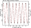 |
Fig. 5. Variations in the measured frequency of the NS rotation due to an orbital motion in the binary system according to the ART-XC data (black points). The model is shown with the dashed red line. |
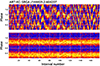 |
Fig. 6. Variations in the phase of pulsations from segment to segment for two folding models. The light curves for each of the segments folded with the period determined for this interval assuming the same epoch time (Tepoch= MJD 60 361.0) (upper panel) and when phase-aligned model is used (bottom panel). |
4.2. Pulse profile evolution
4.2.1. Pulse profiles of the persistent emission
As the first step, we investigated the change in the pulse profile with the flux for the persistent emission. To do this, we used 17 time intervals between successive type I X-ray bursts and folded the 4–25 keV source light curve using the phase-aligned model (see Sect. 4.1). The folded curves are shown in Fig. 7a. We then estimated the pulsed fraction (PF) using a standard expression PF =(Cmax − Cmin)/(Cmax + Cmin), where C is the count rate within the bin, for each of the intervals and traced its value with the flux. The dependence of the PF on the flux in the energy range of 4–25 keV is shown in Fig. 7c. The PF is consistent with being constant at low and medium fluxes, 0.112(4) and 0.113(3), respectively, and it decreases to the value of 0.091(3) at high fluxes. It follows from Fig. 7a that the pulse profiles in a wide energy range differ only very little. Particularly, at lower fluxes, the profile can be described by a sine wave at phases 0.0–0.5 and as a plateau in the range of 0.5–1.0. At higher fluxes, a small bump (interpulse) appears instead of the plateau. To demonstrate the difference more clearly, we made pulse profiles for three flux levels (Fig. 7b). The smaller pulsating fraction in high state is probably due to the presence of the interpulse.
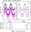 |
Fig. 7. Evolution of the pulse profile (panels a and b) and pulsed fraction (panel c) with the source intensity. |
In the next step, an evolution of the pulsed emission with the energy was investigated. We divided the 4–25 keV energy range of the ART-XC telescope into four bands (4–8, 8–12, 12–17, and 17–25 keV) and reconstructed light curves for all observations in each band, excluding data intervals containing X-ray bursts. We also considered an additional channel of 25–35 keV (technically, the telescope mirrors can focus photons with an energy of up to 35 keV). In a normal situation, this range is not used because the event registration is not efficient and the absolute flux calibrations are difficult, but for a qualitative analysis, it can be quite representative. The resulting pulse profiles in different energy bands are presented in Fig. 8. The pulse shape clearly depends weakly on the energy. Additionally, in all energy ranges, the sine-like wave part is present, while the shape of the plateau is varied. There is also a small but noticeable phase shift Δϕ with energy, with the harder photons arriving earlier than the softer photons, for example, Δϕ = −0.05 for the 17–25 keV photons relative to 4–8 keV photons (i.e., the slope of the linear relation of Δϕ(E) is −0.003(1) keV−1).
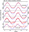 |
Fig. 8. Pulse profiles of the persistent emission from the source in five energy bands. The blue lines show the approximations with a sine wave in the phase interval 0.0–0.5. |
4.2.2. Pulse profiles during X-ray bursts
To track the possible evolution of the pulse profile during the bursts, we divided the bursts into four time intervals counting from the beginning of each burst: 0–3, 3–12, 12–18, and 18–36 s. The left part of Fig. 9 shows the light curve of the source averaged over all X-ray bursts, and the selected intervals are highlighted by different colors. The results of applying the folding procedure to the light curves extracted from these time intervals are shown in the right panels of Fig. 9. In addition, we also provide the folded light curve of the persistent emission of intervals of 1000 s before and after the bursts (the bottom right panel). The pulse profiles practically do not change during the burst and have a sinusoidal shape with a steeper left wing. This shape differs significantly from the shape of the pulse profile of the persistent emission. The fraction of pulsating emission in the 4–25 keV energy range remains constant during the bursts, about 11%, and it is similar to the value of the pulsed fraction for the persistent emission in the same energy band.
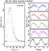 |
Fig. 9. Pulse profile evolution during type I X-ray bursts. The appropriate time intervals are coded by color. The pulse profile of the persistent emission is shown in black in the bottom right panel. |
5. Discussion
We have reported the discovery of SRGA J1444, a new member of a small class of AMXPs. We clearly detected pulsations from the source at a frequency of about 447.9 Hz and determined the binary ephemeris based on the evolution of this frequency over time. Our solution agrees well with the ephemerides obtained from the data of NICER (Ray et al. 2024) and Insight-HXMT (Li et al. 2024) observatories. Based on the ephemeris, it is possible to obtain a pulsar mass function fx ≃ 0.006 M⊙, which in turn gives the estimate for the mass of a normal companion in this system, M2 > 0.25 M⊙ (assuming the NS mass of MNS = 1.4 M⊙).
5.1. Constraints from the burst and persistent X-ray emission
Based on the observational values, we can estimate some parameters of the binary system or accretion flow. In particular, using the peak burst luminosity value, we estimated the distance to the system. When we take the empirical value of the Eddington luminosity (2.2–3.8)×1038 erg s−1, which only depends on the hydrogen abundance in the burst fuel (Kuulkers et al. 2003) and the burst peak bolometric flux Fpk = 2.67 × 10⁻⁸ erg cm−2 s−1, then the upper limit on the distance to the system is D < 8–11 kpc (a more advanced approach is presented in the next section).
Our data provide an opportunity to evaluate another key parameter, the α ratio of accretion to thermonuclear energy, which allowed us to evaluate the composition of the bursting fuel, namely the mean hydrogen fraction at ignition,  . In other words, α shows by how much the efficiency of the energy release during the accretion process is higher than in a thermonuclear reaction, and it can be calculated as the ratio of the energy that is released between two consecutive bursts to the energy that is released per burst. In observational terms, this parameter can be expressed as follows:
where Δt is the burst recurrence time,  is the mean persistent flux between bursts, Cbol is the coefficient to convert the persistent flux from a narrow energy band into bolometric flux, and Eb is the burst fluence (see Galloway et al. 2022, and references there for more details). From the 17 pairs of consecutive bursts, we can estimate the products
  , which are all consistent within the errors with the value 1.468(3)×10−5 erg cm−2 (Fig. 10). We estimated Cbol using the model describing the spectrum of persistent emission and extended the energy range to 0.2–60 keV (in which the vast majority of energy is released). According to the model, the flux in this energy range is about three times higher than the flux in the range 4–25 keV (Cbol = 3). Based on time-resolved spectroscopy of the burst, we calculated the bolometric fluence Eb = 4.18 × 10⁻⁷ erg cm−2. Substituting the values obtained above into Eq. (1), we obtain α ≃ 105. From the measured value of α, we can estimate the hydrogen mass fraction
  in the ignition layer using Eq. (11) in Galloway et al. (2022). We obtain
  assuming an NS radius RNS = 11.2 km and a mass MNS = 1.4 M⊙, indicating that the fuel is rich in helium.
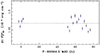 |
Fig. 10. Dependence of the product |

5.2. Spectral evolution of the X-ray bursts
The spectra of X-ray bursting NSs are well fit by a diluted blackbody and can be described by the model spectra of hot NS atmospheres (London et al. 1986; Lewin et al. 1993; Suleimanov et al. 2012). The spectral evolution of X-ray bursts that occurred during the hard persistent spectral state can be described with sequences of model atmosphere spectra of decreasing relative luminosities (Suleimanov et al. 2012; Kajava et al. 2014). In the late burst stages, the atmospheres of the X-ray bursting NSs can be heated by renewed accretion, which leads to certain changes in the emergent spectrum (Suleimanov et al. 2018).
A model of hot NS atmosphere spectra can be approximated by a diluted blackbody (see, e.g., Suleimanov et al. 2011)
where the effective temperature Teff is the parameter of the model atmosphere, w is the dilution factor, and fc is the color-correction factor, c is the speed of light, and h is the Planck constant. The values of w and fc depend on Teff, the surface gravity, and the chemical composition of the atmosphere. Extended tables of w and fc for three chemical compositions (pure He, solar abundance, and solar H/He mix with the metal abundances reduced by a factor of 100), nine surface gravities, and more than 20 relative luminosities were computed using the model atmospheres by Suleimanov et al. (2012). The effective temperature for a given relative luminosity ℓ = L/LEdd depends on the surface gravity and on the chemical composition. The tables of w and fc can be used to interpret the spectral evolution of the X-ray burst after the maximum flux when the observed spectra are fit with a blackbody.
From the parameters of the blackbody fits shown in Fig. 4, we constructed a dependence of the blackbody normalization Kbb (in units (km/10 kpc)2) on the bolometric flux Fbb (in erg cm−2 s−1) (see Figs. 11 and 12). This observed dependence can be fit with a model  using the direct cooling tail method (Suleimanov et al. 2017a). The theoretical models depend on the NS mass MNS and radius RNS, which therefore can be constrained for the given X-ray bursting NS. The observed data for the X-ray bursts of the investigated source are not good enough to use the direct cooling method. Therefore, we fixed the NS mass MNS = 1.5 M⊙ and considered the model curves computed for the fixed surface gravity, log g = 14.3. In this case, we obtained two fitting parameters: the observed Eddington flux FEdd, and the geometrical dilution factor Ω. They depend on the distance to the source D, the NS radius RNS, and the gravitational redshift z at the NS surface,
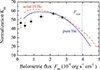 |
Fig. 11. Evolution of the spectral parameters of the averaged X-ray burst from SRGA J1444. The best-fit model curves for solar H/He mix (dashed red curve) and pure He atmospheres (solid blue curve) are shown. The vertical dashed line corresponds to the Eddington flux for a pure He atmosphere model. |
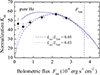 |
Fig. 12. Same as Fig. 11, but showing the best fits to the data with the accretion-heated pure He atmosphere models of various accretion luminosities Lacc/LEdd = 0 (solid line), 0.03 (dotted), and 0.05 (dashed) (Suleimanov et al. 2017a). The vertical dashed line gives the Eddington flux for the model with Lacc/LEdd = 0.03. |
where κT = 0.2(1 + X) cm2 g−1 is the electron-scattering opacity, and X is the hydrogen mass fraction in the atmosphere.
We first tried to describe the data with the models computed for two chemical compositions, pure He and solar H/He mix. The results are presented in Fig. 11 and in the first two columns of Table 1. We note that the obtained distances and the NS radii are only rather rough estimates. However, we can conclude that a pure He composition of the NS atmosphere is preferred because the radius estimate is closer to the commonly accepted values of 11–13 km (Nättilä et al. 2016, 2017; Suleimanov et al. 2017a,b; Abbott et al. 2019; Riley et al. 2021). This conclusion also agrees with the low X obtained on the base of the α value.
Parameters of the NS atmosphere models fit to the spectral evolution of the bursts.
We used only two observational points in the estimates presented above. The deviations of other points from the model curves can be explained by the accretion heating (Suleimanov et al. 2018). Moreover, we can suggest that accretion heats the NS atmosphere during the whole burst duration, because we observe the pulsations during all burst phases (see Fig. 9). Therefore, we tried to fit the observed data with the models computed for pure He, log g = 14.3, and two accretion rates corresponding to Lacc/LEdd = 0.03 and 0.05. The results are presented in Fig. 12 and in the two rightmost columns of Table 1. These fits give even more acceptable NS radii of about 11–12 km. We note, however, that the cooling tail method is based on the assumption that the NS surface emission is uniform. This is not correct for the investigated source, because it shows pulsations during the bursts, and therefore, the obtained estimates are approximate.
5.3. Modeling the pulse profiles
We found that the pulse profiles of the persistent emission of SRGA J1444 have interesting shapes. They exactly follow the sine wave in the phase interval 0.0–0.5 and show a plateau at phases 0.5–1.0 (Fig. 7). The plateau shape also depends on energy to some degree. At high fluxes, a small bump appears in the middle of the plateau (Fig. 8).
The simplest explanation for the observed behavior is that two hotspots (associated with the magnetic poles) contribute to the total emission. At phases 0.0–0.5, only the primary spot, closest to the observer, produces the signal, while at phases 0.5–1.0, there is an additional contribution from the secondary antipodal hotspot. Because of the large compactness, two antipodal spots can be seen together, and when their emission pattern is close to the blackbody, the two sine waves coming out of phase cancel each other and produce a plateau (Beloborodov 2002; Poutanen & Beloborodov 2006).
However, the emission in the ART-XC energy range is clearly not a blackbody, but is produced by Comptonization in an optically thin region (Poutanen & Gierliński 2003). Thus, the emission diagram is different, and it is not then obvious why the pulse profile has a plateau. An alternative explanation involves the effects of a partial eclipse of the secondary (southern) hotspot by the accretion disk (Poutanen et al. 2009). For a stable accretion to proceed, the inner radius of the accretion disk is expected to lie within the corotation radius, which for a 447.9 Hz pulsar is Rco ≈ 29 (MNS/1.4 M⊙)1/3 km. This is just a factor of 2.2 larger than the NS radius. Thus, the line of sight toward the southern magnetic pole can pass through the accretion disk. The eclipse of the secondary hotspot by the disk likely caused a complex evolution of the pulse profiles during the outburst of SAX J1808.4−3658 (Ibragimov & Poutanen 2009; Poutanen et al. 2009; Kajava et al. 2011).
In order to model the pulse profiles, we considered two circular antipodal hotspots at the NS surface, with the primary spot being at a colatitude θ. The angular size of the spot is ρ, the observer inclination relative to the NS spin is i, and the inner radius of the accretion disk is Rin. The angular emission pattern of the intensity of radiation in the spot frame is parameterized through the linear relation I(μ)∝1 + h cos α′, where α′ is the angle relative to the local normal in the spot comoving frame. Parameter h takes the value of 0 for the blackbody emission, while a negative h corresponds to the Comptonized emission from an optically thin slab (Poutanen & Gierliński 2003; Viironen & Poutanen 2004; Bobrikova et al. 2023). For simplicity, we considered a Schwarzschild metric and a spherical shape of the NS surface. We used the code described in Poutanen & Gierliński (2003) and Poutanen & Beloborodov (2006) to model the light curves accounting for disk eclipse following formalism from Ibragimov & Poutanen (2009). We fit the data corresponding to the high state by eye (Fig. 7b). We fixed the NS mass to 1.4 M⊙ and the radius to 12 km. We obtained a good description of the data for the pulsar inclination i = 58°, colatitude of the spot center of 14°and its angular radius of 33°, the inner disk radius of 24.6 km, the anisotropy parameter h = −0.63, and the phase shift of 0.43 (see Fig. 13). We do not provide the errors on the parameters because we did not properly analyze the full parameter space. It is well possible that a reasonably good fit can be obtained with a slightly different set of parameters. However, we note that changing any of the parameters by even 10% leads to a substantial change in the pulse profile that makes it inconsistent with the data. The obtained spot colatitude and the anisotropy parameter are similar to the values estimated from the pulse profiles of SAX J1808.4−3654 (Poutanen & Gierliński 2003; Poutanen et al. 2009), which has a similar PF. The inner disk radius lies within the corotation radius, as expected for a source in accretion phase. Its value is not far from the value of 21.3 km obtained by Poutanen et al. (2009) for SAX J1808.4−3654 when it showed a very similar pulse profile with a plateau.
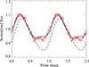 |
Fig. 13. Normalized pulse profiles of the persistent emission of SRGA J1444 during the high state (upper data point at Fig. 7b shown with red crosses) together with an example two-spot model (solid black curve). The dashed curve gives the contribution from the primary spot. |
As we noted above, the pulse profiles during the bursts (Fig. 9) differ substantially from those in the persistent emission. This is very different from other bursting AMXPs, for instance, XTE J1814−338 and MAXI J1816−195 (Strohmayer et al. 2003; Ji et al. 2024), which show nearly identical profiles. As a result, the same two-spot model with the disk eclipses does not reproduce the data. Clearly, some model modifications are required.
6. Summary
We presented the results of the analysis of 133 ks of SRG/ART-XC data, which led to the discovery of a new AMXP, SRGA J1444. Our main results can be summarized as follows:
-
The timing analysis revealed a coherent signal near 447.9 Hz modulated by the Doppler effect due to the orbital motion. The derived parameters for the binary system are consistent with a circular orbit with a period of ∼5.2 h.
-
The pulse profiles of the persistent emission, showing a sine-like part during half a period with a plateau in between, can well be modeled by emission from two circular spots that are partially eclipsed by the accretion disk.
-
Nineteen thermonuclear X-ray bursts were detected during the observations. All bursts have similar shapes and energetics, and none show any signs of a photospheric radius expansion. The X-ray burst recurrence time increases linearly with time from ∼1.6 h at the beginning of observations to ∼2.2 h at the end, and it is anticorrelated with the persistent flux.
-
The spectral evolution during the bursts is consistent with the models of NS atmospheres that are heated by accretion, and it implies an NS radius of 11–12 km and a distance to the source of 8–9 kpc.
-
Pulsations during the bursts were detected. We showed that the pulse profiles differ substantially from those observed in the persistent emission. However, we were unable to find a simple physical model that would explain the pulse profiles detected during the bursts.
After our article was sent to the journal, Ng et al. (2024b) published a more accurate orbital solution, which also showed that the spin period does not change with time. This prompted us to carry out additional calibrations of the onboard clock and make a phase-connected analysis. The newly obtained orbital model (to be published elsewhere) perfectly describes the ART-XC data. Interestingly, this model gives an identical pulse profile shape to that obtained from the phase-alignment model considered here.
Acknowledgments
This work is based on observations with the Mikhail Pavlinsky ART-XC telescope, hard X-ray instrument on board the SRG observatory. The SRG observatory was created by Roskosmos in the interests of the Russian Academy of Sciences represented by its Space Research Institute (IKI) in the framework of the Russian Federal Space Program, with the participation of Germany. The ART-XC team thanks Lavochkin Association (NPOL) with partners for the creation and operation of the SRG spacecraft (Navigator). This work was supported by the Ministry of Science and Higher Education grant 075-15-2024-647. VFS thanks the Deutsche Forschungsgemeinschaft (DFG) for financial support (grant WE 1312/59-1).
References
- Abbott, B. P., Abbott, R., Abbott, T. D., et al. 2019, Phys. Rev. X, 9, 011001 [Google Scholar]
- Arnaud, K. A. 1996, ASP Conf. Ser., 101, 17 [Google Scholar]
- Baglio, M. C., Russell, D. M., Saikia, P., et al. 2024, ATel, 16487, 1 [NASA ADS] [Google Scholar]
- Beloborodov, A. M. 2002, ApJ, 566, L85 [Google Scholar]
- Bobrikova, A., Loktev, V., Salmi, T., & Poutanen, J. 2023, A&A, 678, A99 [NASA ADS] [CrossRef] [EDP Sciences] [Google Scholar]
- Cowie, F. J., Gillanders, J. H., Rhodes, L., et al. 2024, ATel, 16477, 1 [NASA ADS] [Google Scholar]
- Di Salvo, T., & Sanna, A. 2022, ASSL, 465, 87 [NASA ADS] [Google Scholar]
- Galloway, D. K., Johnston, Z., Goodwin, A., & He, C.-C. 2022, ApJS, 263, 30 [NASA ADS] [CrossRef] [Google Scholar]
- Ibragimov, A., & Poutanen, J. 2009, MNRAS, 400, 492 [CrossRef] [Google Scholar]
- Illiano, G., Zelati, F. C., Marino, A., et al. 2024, ATel, 16510, 1 [NASA ADS] [Google Scholar]
- Ji, L., Ge, M., Chen, Y., et al. 2024, ApJ, 596, L67 [Google Scholar]
- Kajava, J. J. E., Ibragimov, A., Annala, M., Patruno, A., & Poutanen, J. 2011, MNRAS, 417, 1454 [NASA ADS] [CrossRef] [Google Scholar]
- Kajava, J. J. E., Nättilä, J., Latvala, O.-M., et al. 2014, MNRAS, 445, 4218 [NASA ADS] [CrossRef] [Google Scholar]
- Kuulkers, E., den Hartog, P. R., in’t Zand, J. J. M., et al. 2003, A&A, 399, 663 [NASA ADS] [CrossRef] [EDP Sciences] [Google Scholar]
- Lewin, W. H. G., van Paradijs, J., & Taam, R. E. 1993, Space Sci. Rev., 62, 223 [CrossRef] [Google Scholar]
- Li, Z., Kuiper, L., Falanga, M., et al. 2024, ATel, 16548, 1 [Google Scholar]
- London, R. A., Taam, R. E., & Howard, W. M. 1986, ApJ, 306, 170 [Google Scholar]
- Mariani, I., Motta, S., Baglio, M. C., et al. 2024, ATel, 16475, 1 [NASA ADS] [Google Scholar]
- Mereminskiy, I. A., Semena, A. N., Molkov, S. V., et al. 2024, ATel, 16464, 1 [NASA ADS] [Google Scholar]
- Nättilä, J., Steiner, A. W., Kajava, J. J. E., Suleimanov, V. F., & Poutanen, J. 2016, A&A, 591, A25 [CrossRef] [EDP Sciences] [Google Scholar]
- Nättilä, J., Miller, M. C., Steiner, A. W., et al. 2017, A&A, 608, A31 [NASA ADS] [CrossRef] [EDP Sciences] [Google Scholar]
- Negoro, H., Mihara, T., Serino, M., et al. 2024, ATel, 16483, 1 [NASA ADS] [Google Scholar]
- Ng, M., Sanna, A., Strohmayer, T. E., et al. 2024a, ATel, 16474, 1 [NASA ADS] [Google Scholar]
- Ng, M., Ray, P. S., Sanna, A., et al. 2024b, ApJ, 968, L7 [NASA ADS] [CrossRef] [Google Scholar]
- Patruno, A., & Watts, A. L. 2021, ASSL, 461, 143 [NASA ADS] [Google Scholar]
- Pavlinsky, M., Tkachenko, A., Levin, V., et al. 2021, A&A, 650, A42 [EDP Sciences] [Google Scholar]
- Poutanen, J., & Gierliński, M. 2003, MNRAS, 343, 1301 [NASA ADS] [CrossRef] [Google Scholar]
- Poutanen, J., & Beloborodov, A. M. 2006, MNRAS, 373, 836 [NASA ADS] [CrossRef] [Google Scholar]
- Poutanen, J., Ibragimov, A., & Annala, M. 2009, ApJ, 706, L129 [NASA ADS] [CrossRef] [Google Scholar]
- Ray, P. S., Strohmayer, T. E., Sanna, A., et al. 2024, ATel, 16480, 1 [NASA ADS] [Google Scholar]
- Riley, T. E., Watts, A. L., Ray, P. S., et al. 2021, ApJ, 918, L27 [CrossRef] [Google Scholar]
- Russell, T. D., Carotenuto, F., Eijnden, J. V. D., et al. 2024, ATel, 16511, 1 [NASA ADS] [Google Scholar]
- Saikia, P., Russell, D. M., Baglio, M. C., et al. 2024, ATel, 16489, 1 [NASA ADS] [Google Scholar]
- Sanchez-Fernandez, C., Kuulkers, E., Ferrigno, C., & Chenevez, J. 2024, ATel, 16485, 1 [NASA ADS] [Google Scholar]
- Sguera, V., & Sidoli, L. 2024, ATel, 16493, 1 [NASA ADS] [Google Scholar]
- Sokolovsky, K., Korotkiy, S., & Zalles, R. 2024, ATel, 16476, 1 [NASA ADS] [Google Scholar]
- Strohmayer, T. E., Markwardt, C. B., Swank, J. H., & in’t Zand, J. 2003, ApJ, 596, L67 [NASA ADS] [CrossRef] [Google Scholar]
- Suleimanov, V., Poutanen, J., & Werner, K. 2011, A&A, 527, A139 [NASA ADS] [CrossRef] [EDP Sciences] [Google Scholar]
- Suleimanov, V., Poutanen, J., & Werner, K. 2012, A&A, 545, A120 [NASA ADS] [CrossRef] [EDP Sciences] [Google Scholar]
- Suleimanov, V. F., Poutanen, J., Nättilä, J., et al. 2017a, MNRAS, 466, 906 [Google Scholar]
- Suleimanov, V. F., Kajava, J. J. E., Molkov, S. V., et al. 2017b, MNRAS, 472, 3905 [NASA ADS] [CrossRef] [Google Scholar]
- Suleimanov, V. F., Poutanen, J., & Werner, K. 2018, A&A, 619, A114 [NASA ADS] [CrossRef] [EDP Sciences] [Google Scholar]
- Sunyaev, R., Arefiev, V., Babyshkin, V., et al. 2021, A&A, 656, A132 [NASA ADS] [CrossRef] [EDP Sciences] [Google Scholar]
- Viironen, K., & Poutanen, J. 2004, A&A, 426, 985 [NASA ADS] [CrossRef] [EDP Sciences] [Google Scholar]
All Tables
Parameters of the NS atmosphere models fit to the spectral evolution of the bursts.
All Figures
|
Fig. 1. Temporal evolution of the SRGA J1444 emission during the 2024 outburst. Upper panel: ART-XC light curve during two observations. The time and mean flux of the type I X-ray bursts are shown with the dashed line and thick streak. Bottom left: Flux evolution as observed by MAXI/GSC in the 4–10 keV energy band. Bottom right: X-ray burst recurrence time (in black, left axis) and the mean persistent flux between the bursts in the 4–25 keV energy band |
| In the text | |
|
Fig. 2. Average energy spectrum of all type I X-ray bursts observed by ART-XC during the first observation (blue crosses) and the spectrum of the persistent emission extracted between bursts II and III (red crosses). The pink curves represent the spectral model of the absorbed blackbody and the cutoff power law. |
| In the text | |
|
Fig. 3. Light curves of all detected type I X-ray bursts in the 4–25 keV energy band. The bottom panel shows the averaged burst profile. The dashed vertical lines represent the time intervals we used for the time-resolved spectral analysis (see Sect. 3.2). |
| In the text | |
|
Fig. 4. Time-resolved spectroscopy of the averaged X-ray burst emission. The dotted blue line in the bottom panel shows the rescaled in amplitude count-rate light curve in 4–25 keV to match the measured fluxes. The pre-burst rate is subtracted. |
| In the text | |
|
Fig. 5. Variations in the measured frequency of the NS rotation due to an orbital motion in the binary system according to the ART-XC data (black points). The model is shown with the dashed red line. |
| In the text | |
|
Fig. 6. Variations in the phase of pulsations from segment to segment for two folding models. The light curves for each of the segments folded with the period determined for this interval assuming the same epoch time (Tepoch= MJD 60 361.0) (upper panel) and when phase-aligned model is used (bottom panel). |
| In the text | |
|
Fig. 7. Evolution of the pulse profile (panels a and b) and pulsed fraction (panel c) with the source intensity. |
| In the text | |
|
Fig. 8. Pulse profiles of the persistent emission from the source in five energy bands. The blue lines show the approximations with a sine wave in the phase interval 0.0–0.5. |
| In the text | |
|
Fig. 9. Pulse profile evolution during type I X-ray bursts. The appropriate time intervals are coded by color. The pulse profile of the persistent emission is shown in black in the bottom right panel. |
| In the text | |
|
Fig. 10. Dependence of the product |
| In the text | |
|
Fig. 11. Evolution of the spectral parameters of the averaged X-ray burst from SRGA J1444. The best-fit model curves for solar H/He mix (dashed red curve) and pure He atmospheres (solid blue curve) are shown. The vertical dashed line corresponds to the Eddington flux for a pure He atmosphere model. |
| In the text | |
|
Fig. 12. Same as Fig. 11, but showing the best fits to the data with the accretion-heated pure He atmosphere models of various accretion luminosities Lacc/LEdd = 0 (solid line), 0.03 (dotted), and 0.05 (dashed) (Suleimanov et al. 2017a). The vertical dashed line gives the Eddington flux for the model with Lacc/LEdd = 0.03. |
| In the text | |
|
Fig. 13. Normalized pulse profiles of the persistent emission of SRGA J1444 during the high state (upper data point at Fig. 7b shown with red crosses) together with an example two-spot model (solid black curve). The dashed curve gives the contribution from the primary spot. |
| In the text | |
Current usage metrics show cumulative count of Article Views (full-text article views including HTML views, PDF and ePub downloads, according to the available data) and Abstracts Views on Vision4Press platform.
Data correspond to usage on the plateform after 2015. The current usage metrics is available 48-96 hours after online publication and is updated daily on week days.
Initial download of the metrics may take a while.