© The Authors 2024

1. Introduction

The concept of coronal heating is tightly linked to wave dynamics. The fact of the matter is that the temperature jump from the solar photosphere to the solar corona is not just a simple gradual elevation process. This rapid temperature enhancement roots in the physics of magnetohydrodynamic (MHD) waves. Studying MHD waves is important because of the presence of magnetic fields within the solar atmosphere, which make the existence of MHD waves possible. Overall, MHD waves are driven by the tension and in general by gradients of the plasma pressure and magnetic pressure (Goossens 2003). Furthermore, MHD waves in the solar atmosphere experience various physical processes that may either lead to damping or amplification, thereby enhancing our knowledge of the coronal heating process across all its aspects.

One particular feature in the solar atmosphere that enables us to study various aspects of MHD waves are solar atmospheric magnetic plasma structures that host all types of MHD waves. By focusing on MHD oscillations especially in loops, jets, or plumes from their origin to their damping, basic and practical physics is bound to be extracted. This facilitates the diagnostics of solar atmospheric plasmas, laying the groundwork for coronal seismology. Before proceeding, it is worth pointing out a selection of observations regarding MHD waves in solar atmospheric plasma structures. For instance, kink oscillations were observed using the imaging telescope on board the TRACE spacecraft in a loop length about 130 × 10⁶ m and diameter about 2 × 10⁶ m (Nakariakov et al. 1999). Furthermore, using the SDO/AIA it was noticed that the period of kink oscillations scales with the loop lengths (Goddard et al. 2016). Nonetheless these waves experience damping by various physical processes, for instance, resonant absorption (Goossens et al. 1992; Terradas et al. 2006). It is worth noting that the driver of kink oscillations is an interesting aspect of MHD wave dynamics, which (from a statistical point of view) is suggested to be due to neighbouring eruptions that deviate loop positions from their equilibrium (Goddard et al. 2016). Meanwhile, Ruderman & Petrukhin (2021) suggested a model with either random or harmonic wave drivers; however, the study of wave drivers requires further focus (Vasheghani Farahani et al. 2009; Mandal et al. 2022). Regarding coronal plumes, it has been shown that the damping of propagating slow waves is dependent on the wave-length and, hence, the frequency. In a sense, this suggests that shorter-period oscillations experience longer damping lengths (Mandal et al. 2018). Magnetoacoustic slow waves (Edwin & Roberts 1983) that are either standing (e.g. Pant et al. 2017) or propagating (e.g. Duckenfield et al. 2021; Arregui et al. 2023) have been observed in loops as well as in multi-mode, using EIS/Hinode and AIA/SDO, and experiencing damping (Wang et al. 2009; Krishna Prasad et al. 2012). The damping effect could be due to anisotropic thermal conduction (Mandal et al. 2016). However, it is always of interest to elucidate the mechanisms resulting in the damping or amplification of waves (Pourjavadi et al. 2021; Riedl et al. 2021). Kohutova et al. (2020) presented an alternate Doppler shift propagating outward of the solar surface at the speed about 140 km/s in an erupting prominence and interpreted it as a torsional wave.

In the context of the present study, focus is being put on the interplay of damping actors and non-linear effects connected to torsional Alfvén waves propagating in solar atmospheric plumes. The observed transverse MHD waves in coronal plumes have also been reported to contribute towards coronal heating and solar wind acceleration (Banerjee et al. 2009; Thurgood et al. 2014). The energy flux associated with damping Alfvén waves in polar coronal holes has a decay rate while elevating upwards, which has been shown to be an adequate candidate for coronal heating (Bemporad & Abbo 2012). However, it is not yet fully known up to what extent MHD waves propagating in open magnetic flux tubes are able to interact with the solar atmosphere (Cranmer 2009); however, their main contribution towards coronal heating takes place at lower altitudes in coronal holes (Hahn et al. 2012).

Alfvén waves experience shocks in the non-linear regime (Gruszecki et al. 2011; Farahani et al. 2021). Since shocks are connected with energy transfer (Houston et al. 2020), Alfvén wave shocks serve as fine agents for the study of magnetic energy, representing a sort of energy dissipation process contributing towards coronal heating. Prior to the present study, a series of models regarding Alfvén wave propagation in various solar magnetic structures were proposed, each of which has, in turn, elevated our knowledge of the character of Alfvén waves, besides their simply having seismological aspects (Nakariakov 2004; Stepanov et al. 2012). The dissipation factors that are specifically examined in the present study are viscosity and stratification. This is due to the fact that with regard to longitudinal waves, the consideration of stratification for instance in loops causes an additional reduction of the damping time from 10–20 percent in comparison to the case where only plasma viscosity is taken under consideration (Mendoza-Briceño et al. 2004). Since loop length enables thermal and dissipative effects to enhance the dissipation rates of longitudinal magnetoacoustic waves that are compressive, a question arises regarding the scaling behaviour of the dissipative processes; in particular, this behaviour is in addition to amplification processes of Alfvén waves, which are transverse and in-compressive in the linear regime (Van Doorsselaere et al. 2008) but do perturb the magnetic flux tube density in the non-linear regime (e.g. Vasheghani Farahani et al. 2011; Vasheghani Farahani & Hejazi 2017; Ghoraba & Farahani 2018).

Before proceeding it is interesting to note that the perpendicular profile considered in the present study is given by a step function, which excludes the effect of phase mixing (e.g. Ruderman & Petrukhin 2018; McMurdo et al. 2023) in the linear regime (Boocock & Tsiklauri 2022). However, the dependence of the phase speed of a torsional wave on the amplitude, while experiencing a density variation near the flux tube boundary may lead to the non-linear phase mixing (Shestov et al. 2017). This effect is out of scope of the present paper due to the fact that it addresses long-wavelength torsional waves. It must also be pointed out that the parallel structuring may significantly enhance the damping of phase-mixed Alfvén waves (Ruderman et al. 1998). This effect is excluded from the current study because of the step-function perpendicular profile.

A theoretical study carried out by Ruderman & Roberts (2002) represented a solar loop in coronal conditions as an initially magnetoacoustic wave transferred its energy to transverse waves (Zaqarashvili 2003), where an explicit relation for the damping time was obtained. Although the loop was considered dissipative in the sense of viscosity, the damping process has been mainly directed towards resonant absorption taking place in the resonant layer (Goossens et al. 1992; Ofman & Davila 1995); this is mainly due to inhomogeneities observed in the loop (Ruderman & Roberts 2002). The inhomogeneities in solar loops cause variations in the Alfvén frequency that may result in coronal heating (Zaqarashvili & Murawski 2007). The question that arises is related to the non-linear regime, where the torsional Alfvén wave experiences wave steeping resulting in shocks (Vasheghani Farahani et al. 2012; Farahani et al. 2021), and considers how damping and amplitude amplification would interplay. The answer to this question would shed light on the scale in which the distributed energy associated with Alfvén waves in solar magnetic cylindrical structures contributes towards coronal heating.

The context of the present study and associated model represented here is inspired by a series of studies regarding the propagation and damping of slow magnetoacoustic waves in coronal plumes (Ofman et al. 2000) and Alfvén waves (Nakariakov et al. 2000) in coronal holes using spherical coordinates. This investigation is informed by studies carried out by Vasheghani Farahani et al. (2012), Ghoraba & Farahani (2018),; Farahani et al. (2021), regarding the non-linear torsional wave propagation in solar magnetic cylindrical structures, using the second order thin flux tube approximation (Zhugzhda 1996). The interest in Nakariakov et al. (2000) is focussed on non-linear Alfvén wave propagation in coronal holes; hence, only parallel structuring has been taken into consideration. These studies showed that when the wave periods are less than 300 s the deviation of the amplitudes of physical perturbations in the non-linear regime differs from that in the linear regime at around eight solar radii. The fact of the matter is that the deviation from the linear regime is dependent on the wave amplitude and period. Meanwhile, the wave steepening due to non-linear effects is reduced 20 percent for an increase of viscosity by as much as an order of magnitude. In the present study, since solar plumes are of main interest, in addition to parallel structuring, transverse structuring needs also to be considered. Regarding Vasheghani Farahani et al. (2012) and Farahani et al. (2021), by only considering transverse structuring the aim was studying the non-linear cascade regarding torsional Alfvén waves in ideal loops or jets. Ghoraba & Farahani (2018) employed the second-order thin flux tube approximation in the ideal regime in the non-linear regime, with only transverse structuring in terms of the application to loops and jets; however, their aim was to highlight the interplay of equilibrium twist and rotation on the physical perturbations. Mozafari Ghoraba et al. (2018) used the second-order thin flux tube approximation with transverse structuring in the application to loops or jets in the presence of viscosity and gravity and obtained an analytic dispersion relation enabling a direct understanding on the effects of equilibrium conditions besides the resistive terms, but the results where limited to the linear case.

In Sects. 2 and 3, the MHD theory, model, and equilibrium conditions applicable to coronal plumes are presented. In Sect. 4, we describe how we obtained the evolutionary equations to provide insights into the resistive and structural effects, in addition to the non-linear effects on the perturbations of the physical variables. In Sect. 5, the results are discussed based on the snapshots extracted from the parametric studies connected with the governing equations, followed by conclusions regarding the scaling behaviour of shock formation and energy transfer in the context of coronal seismology in Sect. 6.

2. Theory and MHD set of equations

The solar atmosphere is structured both along and across the background magnetic field. To provide a model of the Alfvén wave shocks in coronal plumes that contributes to coronal heating besides the dissipative terms, the second-order thin flux tube approximation (Zhugzhda 1996; Zhugzhda & Nakariakov 1999; Vasheghani Farahani et al. 2010) in the context of MHD theory was applied to the resistive MHD set of equations (Goossens 2003), where we have (Mozafari Ghoraba et al. 2018):

$$\begin{array}{c}\hfill \frac{\partial \mathrm{\Omega }}{\partial t}+2\mathrm{\Omega }V+u\frac{\partial \mathrm{\Omega }}{\partial z}+\frac{J}{4\pi \rho }\frac{\partial B_z}{\partial z}-\frac{B_z}{4\pi \rho }\frac{\partial J}{\partial z}-\nu \frac{{\partial }^2\mathrm{\Omega }}{\partial z^2}=0,\end{array}$$(1)

$$\begin{array}{cc}& \rho (\frac{\partial u}{\partial t}+u\frac{\partial u}{\partial z})+\frac{\partial P}{\partial z}-\frac{4}{3}\rho \nu \frac{{\partial }^{2}u}{\partial z^2}-\frac{2}{3}\rho \nu \frac{\partial V}{\partial z}+g\rho \hfill \\ \hfill & =-\frac{R^2}{4\pi }J\frac{\partial J}{\partial z},\hfill \end{array}$$(2)

$$\begin{array}{cc}& P+\frac{B_z^2}{8\pi }-\frac{A}{2\pi }[\rho (\frac{\partial V}{\partial t}+u\frac{\partial V}{\partial z}+V^2-{\mathrm{\Omega }}^2-\nu \frac{{\partial }^{2}V}{\partial z^2})\hfill \\ \hfill & +\frac{1}{4\pi }(J^2+\frac{B_z}{2}\frac{{\partial }^2{B}_z}{\partial z^2}-\frac{1}{4}{\left(\frac{\partial B_z}{\partial z}\right)}^2)]=P_T^{\mathrm{ext}},\hfill \end{array}$$(3)

$$\begin{array}{c}\hfill \frac{\partial \rho }{\partial t}+2\rho V+\frac{\partial \left(\rho u\right)}{\partial z}=0,\end{array}$$(4)

$$\begin{array}{c}\hfill \frac{\partial J}{\partial t}+\frac{\partial (uJ)}{\partial z}-B_z\frac{\partial \mathrm{\Omega }}{\partial z}+2JV=0,\end{array}$$(5)

$$\begin{array}{c}\hfill \frac{\partial B_z}{\partial t}+u\frac{\partial B_z}{\partial z}+2B_{z}V=0,\end{array}$$(6)

$$\begin{array}{c}\hfill (\frac{\partial }{\partial t}+u\frac{\partial }{\partial z})\frac{P}{{\rho }^{\gamma }}=0.\end{array}$$(7)

Here, Ω represents the vorticity and J stands for the current density of the plume at a radius, r, which is the radial distance from the plume axis. The plasma density is denoted by ρ, while P represents the gas pressure. Additionally, $P_T^{\mathrm{ext}}$ signifies the external total pressure and V corresponds to the radial derivative of the radial component of the velocity. The radial and axial components of the velocity and magnetic field intensity are represented by u and B_z, respectively. The parameter g denotes the solar gravity acceleration while the cross-sectional area of the plume is denoted by A. Finally, we use ν to represent the kinematic viscosity and γ to denote the adiabatic index of the system. It is instructive to note that in case where the parallel structuring is absent and the perturbations of the external medium are neglected, besides complying with ideal conditions; Eqs. (1)–(7) are simplified to Eq. (3) of Vasheghani Farahani et al. (2010). It is worth noting that as of the series of studies prior to the present study concerning torsional Alfvén wave propagation in solar twisted magnetic cylindrical structures where we have axial symmetry, (∂/∂φ = 0), the zeroth-order value for the current density, J, is utilised in place of the azimuthal magnetic field divided by the tube radius, (B_φ/r), while the zeroth-order value for the vorticity, Ω, is employed instead of the azimuthal velocity divided by the tube radius, (V_φ/r), as in, for instance, Vasheghani Farahani et al. (2010).

3. Model and equilibrium conditions

To model a coronal plume hosting Alfvén waves, consider an initially static plume embedded in a static medium where the equilibrium density and plasma pressure internal and external to the plume are respectively represented by ρ₀, p₀ and ρ_0e, p_0e. Meanwhile, the equilibrium magnetic fields internal and external to the plume are parallel to the plume axis, respectively, represented by B_z0 and B_z0e. Now, by complying with the pressure balance at the plume boundary together with the radial velocity continuity at the tube boundary, we obtain:

$$\begin{array}{c}\hfill \begin{array}{cc}& \frac{\partial \mathrm{\Omega }}{\partial t}-\frac{B_0(z)}{4\pi {\rho }_{{}_0}(z)}\frac{\partial J}{\partial z}-\nu \frac{{\partial }^2\mathrm{\Omega }}{\partial z^2}\hfill \\ \hfill & =\frac{B_0(z)}{4\pi {\rho }_{{}_0}(z)}[\frac{B_z}{B_0(z)}-\frac{\rho }{{\rho }_{{}_0}(z)}]\frac{\partial J}{\partial z}-2V\mathrm{\Omega }\hfill \\ \hfill & -u\frac{\partial \mathrm{\Omega }}{\partial z}-\frac{J}{4\pi {\rho }_{{}_0}(z)}\frac{\partial B_z}{\partial z},\hfill \end{array}\end{array}$$(8)

$$\begin{array}{cc}\hfill {\rho }_{{}_0}(z)\frac{\partial u}{\partial t}& +C_s^2\frac{\partial \rho }{\partial z}-\frac{4}{3}{\rho }_{{}_0}(z)\nu (\frac{{\partial }^{2}u}{\partial z^2}-\frac{1}{2}\frac{\partial V}{\partial z})\hfill \\ \hfill & =-g\rho -\frac{R^2}{4\pi }J\frac{\partial J}{\partial z},\hfill \end{array}$$(9)

$$\begin{array}{c}\hfill \begin{array}{cc}& P+\frac{B_0(z)B_z}{4\pi }-\frac{A_0{\rho }_{{}_0}(z)}{2\pi }[\frac{\partial V}{\partial t}-\nu \frac{{\partial }^{2}V}{\partial z^2}+\frac{B_0(z)}{8\pi {\rho }_{{}_0}(z)}\frac{{\partial }^2{B}_z}{\partial z^2}]\hfill \\ \hfill & ={\kappa }^2\rho +\frac{A_0}{8{\pi }^2}{J}^2-\frac{A_0{\rho }_{{}_0}(z)}{2\pi }{\mathrm{\Omega }}^2,\hfill \end{array}\end{array}$$(10)

$$\begin{array}{c}\hfill \frac{\partial \rho }{\partial t}+2{\rho }_{{}_0}(z)V+{\rho }_{{}_0}(z)\frac{\partial u}{\partial z}=0,\end{array}$$(11)

$$\begin{array}{c}\hfill \frac{\partial J}{\partial t}-B_0(z)\frac{\partial \mathrm{\Omega }}{\partial z}=B_z\frac{\partial \mathrm{\Omega }}{\partial z}-\frac{\partial }{\partial z}(Ju)-2JV,\end{array}$$(12)

$$\begin{array}{c}\hfill \frac{\partial B_z}{\partial t}+2B_0(z)V=0,\end{array}$$(13)

where A₀ represents the area of the plume at equilibrium. An interesting aspect of Eqs. (8)–(13) is that for conditions where the perturbations of external pressure and parallel structuring are not of interest and ideal conditions apply; they simplify to the set equations expressed in Vasheghani Farahani et al. (2011) and Vasheghani Farahani et al. (2012), where the aim of those studies was to find the induced frequencies, density saturation, and non-linear cascade.

It is noteworthy that the perturbation of the total pressure in the external medium, $P_T^{\mathrm{ext}}$, can be derived from the gas pressure, magnetic pressure, and the plasma-β of the external medium, serving as terms within the compressive perturbations inside the flux tube as:

$$\begin{array}{c}\hfill P_T^{\mathrm{ext}}={\kappa }^2{\rho }_{\mathrm{in}},\end{array}$$(14)

where the parameter κ represents the physical matching coefficient in a velocity scale, elucidating the relationship between external pressure and internal density, expressed as:

$$\begin{array}{c}\hfill {\kappa }^2=\frac{\chi C_{\mathrm{se}}^2({\beta }_{\mathrm{ext}}+1)}{{\beta }_{\mathrm{ext}}}.\end{array}$$

where we have χ = ρ_ext/ρ_in, β_ext = 2C_se²/γC_Ae², while C_se is the external sound speed. The parameter κ is obtained by complying with the continuity of the pressure balance at the plume boundary together with the continuity of the Lagrangian displacement at the plume boundary (Vasheghani Farahani et al. 2017). The most interesting aspect of Eq. (14) is because it provides understanding on how the plume boundary is balanced based on the total pressure external and the density internal to the plume, see also Vasheghani Farahani et al. (2017) and Farahani et al. (2021). In other words, it expresses the external total pressure based on the plume density, which itself acts as an important tool for coronal seismology.

It is imperative to note that Eqs. (8)–(13) are generalisations of the equations presented in Vasheghani Farahani et al. (2011) and Vasheghani Farahani et al. (2012). Interestingly, the model studied by Ghoraba & Farahani (2018) dealt with initially non-static jets in the linear regime concerning the impact of compressible and shear viscosity on torsional fast magnetoacoustic waves in the solar atmosphere. However, their aim was to study the effects of viscosity on the interplay of the equilibrium twist and rotation on the phase speed of the fast magnetoacoustic waves and hence their damping. The gravity in their study was also taken as a constant value without depending on height and consequently the equilibrium density was considered constant. In contrast, in the present study, the effects connected with the varying gravity with respect to the height as parallel structuring (Nakariakov et al. 2000) is of particular interest, in addition to the second thin flux tube approximation of transverse structuring (Edwin & Roberts 1983) in the non-linear regime for a coronal hole plumes. This is while for coronal holes studied by Nakariakov et al. (2000), only parallel structuring was needed. The profile for the stratification under consideration in the present study is also based on the profile presented by Nakariakov et al. (2000), as follows:

$$\begin{array}{c}\hfill {\rho }_{{}_0}(z)={\rho }_{{}_0}(0)\exp (-\frac{R_{\odot }}{H}\frac{z}{z+R_{\odot }})\equiv {\rho }_{{}_0},\end{array}$$(15)

where the R_⊙ is the solar radius and H represents the height scale. It is assumed that the atmosphere is isothermal, maintaining a constant temperature denoted as T, along with a sound speed denoted as C_s. Both the height scale, H, and sound speed, C_s, are contingent upon the temperature, T. In the solar corona, approximate relationships are employed: H(Mm) = 50T(MK) and $C_s({\mathrm{Mms}}^{-1})=0.152T^{\frac{1}{2}}(\mathrm{MK})$. It is important to note that this model is applicable to coronal plumes where the temperature is considered to be constant with altitude. The equilibrium magnetic field B₀ is presumed to be locally strictly vertical to the solar surface and is governed by:

$$\begin{array}{c}\hfill B_0(z)=\frac{B_0(0)R_{\odot }^2}{{(z+R_{\odot })}^2}\equiv B_0.\end{array}$$(16)

To ensure the divergence of the background magnetic field (Eq. (16)) is equal to zero and to make sure the magnetic flux is conserved, the cross-sectional area of the flux tube, denoted as A₀, is then determined as:

$$\begin{array}{c}\hfill A_0(z)=A_0(0){(1+\frac{z}{R_{\odot }})}^2\equiv A_0.\end{array}$$(17)

The equilibrium tube area, A₀(z), is defined as πR(z)², where R(z) represents the radius of the plume and is varying with respect to height from the solar surface as

$$\begin{array}{c}\hfill R(z)=R_0(1+\frac{z}{R_{\odot }})\equiv R,\end{array}$$(18)

where R₀ is the radius of the flux tube at the base of the corona. Equations (15) and (16) yield the longitudinal profile of the Alfvén speed, C_A:

$$\begin{array}{c}\hfill C_{{}_A}(z)=\frac{B_0(0)R_{\odot }^2}{{(z+R_{\odot })}^2{[4\pi {\rho }_{{}_0}(0)]}^{\frac{1}{2}}}\exp \left(\frac{R_{\odot }}{2H}\frac{z}{z+R_{\odot }}\right)\equiv C_{{}_A}.\end{array}$$(19)

In typical coronal scenarios, the temperature, T, hovers around 1.0–1.4 MK, thereby resulting in H ≪ R_⊙. Equations (15), (16), and (19) represent the cylindrical mutual expressions corresponding to Eqs. (1)–(3) of Nakariakov et al. (2000). In Fig. 1(a), the profile of the stratified Alfvén speed is depicted, whereas Fig. 1(b) shows the tube speed versus the normalized altitude by the radius of the sun, R_⊙. Figure 1(c) illustrates how the cross-section of the tube expands within the stratified plasma modelled in this article to height. As for Eqs. (15)–(19), in the subsequent calculations and formulas, ρ₀, B₀, A₀, R, and C_A are used as a shorthand notation for ρ₀(z), B₀(z), A₀(z), R(z), and C_A(z), respectively.

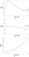Fig. 1. Vertical profiles of the equilibrium properties of a waveguiding magnetic flux tube based on the stratified density and magnetic field intensity models described by Eqs. (15) and (16). (a) Stratified Alfvén speed (CA(z)) inside the flux tube (Eq. (19)) with maximum at around 1.5 solar radii. (b) Stratified tube speed inside the flux tube $(C_{{}_T}(z)\equiv \frac{C_A^2{C}_s^2}{C_A^2+C_s^2})$. (c) Profile of the normalized equilibrium cross-section of the flux tube (Eq. (17)) relative to the tube cross-section at the base of the corona $\left(\frac{A_0(z)}{A_0(0)}\right)$, as a function of height which is normalized by the radius of the sun. The Alfvén speed near the corona’s base is 1000 km/s.

4. Wave equation for stratified coronal hole plumes

In this study, we solely focus on shear viscosity, even though compressive viscosity is considered in the perturbed equations. The reason is that the compressive part of the viscosity affects Alfvén waves through the compressive perturbations induced non-linearly; as the non-linearity is assumed to be weak, its impact is expected to be weak and thus negligible. Moreover, non-linear effects are presumed to be weak (B_φ/B₀ ≪ 1) and we confined the derivation to short wavelength motions; specifically, λ ≪ H. This enables us to consider the effect of stratification as weak perturbations as well. As such by implementing Eqs. (8)–(13) the non-linear effects connected with the Alfvén wave propagation on the density perturbations of the tube could be obtained as:

$$\begin{array}{c}\hfill \begin{array}{cc}& (C_{{}_A}^2+C_{{}_S}^2)D_{{}_T}\rho +\frac{A_0}{4\pi }{D}_{{}_A}{D}_{{}_S}\rho -{\kappa }^2\frac{{\partial }^2\rho }{\partial t^2}\hfill \\ \hfill & =\frac{A_0}{2\pi }\frac{{\partial }^2}{\partial t^2}(\frac{J^2}{4\pi }-{\rho }_0{\mathrm{\Omega }}^2)+\frac{R^2{C}_{{}_A}^2}{4\pi }\frac{\partial }{\partial z}\left(J\frac{\partial J}{\partial z}\right),\hfill \end{array}\end{array}$$(20)

where

$$\begin{array}{c}\hfill D_{{}_{T,S,A}}=\frac{{\partial }^2}{\partial t^2}-C_{{}_{T,S,A}}^2\frac{{\partial }^2}{\partial z^2},C_{{}_T}^2=\frac{C_{{}_A}^2{C}_{{}_S}^2}{C_{{}_A}^2+C_{{}_S}^2},C_{{}_A}=\frac{B_{{}_0}}{\sqrt{4\pi {\rho }_{{}_0}}}.\end{array}$$(21)

Equation (20) enables a qualitative understanding on the signature of the non-linear effects connected with the torsional Alfvén wave, namely, J and Ω on the density, which represents compressive perturbation. When the context of study is focused only on the plasma internal to the plume with lack of external interference, the third term on the LHS of Eq. (20) disappears. The outcome aligns with Eq. (15) of Vasheghani Farahani et al. (2012). On the other hand, the equation corresponding to Eq. (20) in the context of solar jets is Eq. (6) from Farahani et al. (2021). By deeming the effects of stratification and weak non-linearity, we can employ the method of slow-varying amplitudes, facilitating the transition to a moving frame of reference through the following variables:

$$\begin{array}{c}\hfill \xi =z,\tau =t-{\displaystyle \int \frac{\mathit{dz}}{C_{{}_A}}},\end{array}$$(22)

where the parameter ξ is a representative for the slowly varying small spatial scale of the system, which is associated with the non-linearity and inhomogeneity of the plasma. Also, τ represents the temporal non-linear scale of the system and C_A is a shorthand notation for C_A(z).

Given the linear relationship between the incompressible parameters, vorticity (Ω), and magnetic twist (J), we may utilise the linear form of Eq. (12) and apply the relations expressing the changing variables (Eq. (22)), resulting in:

$$\begin{array}{c}\hfill J=-\frac{B_{{}_0}}{C_{{}_A}}\mathrm{\Omega }.\end{array}$$(23)

By applying the changing variables Eq. (22) and the use of the relation Eq. (23) to Eq. (20), we provide a relation that expresses the direct effects connected with the Alfvén wave in the non-linear regime represented by the vorticity (Ω) on the compressive perturbations of the coronal plume as

$$\begin{array}{c}\hfill \rho =\frac{R^2{B}_0^2}{8\pi C_{{}_A}^2(C_{{}_A}^2-{\kappa }^2)}{\mathrm{\Omega }}^2.\end{array}$$(24)

Hence, the effects connected with the vorticity, which is the signature of the Alfvén wave in the context of the present study, could readily be obtained from the set equations numbered between (8)–(13) and Eq. (24) as:

$$\begin{array}{c}\hfill \begin{array}{cc}\hfill u& =\frac{R^2(C_{{}_A}^2+C_{{}_S}^2-{\kappa }^2)}{2C_{{}_A}(C_{{}_A}^2-{\kappa }^2)}{\mathrm{\Omega }}^2,V=\frac{R^2(C_{{}_S}^2-{\kappa }^2)}{4C_{{}_A}^2(C_{{}_A}^2-{\kappa }^2)}\frac{\partial {\mathrm{\Omega }}^2}{\partial \xi },\hfill \\ \hfill B_z& =\frac{-R^2{B}_0(C_{{}_S}^2-{\kappa }^2)}{2C_{{}_A}^2(C_{{}_A}^2-{\kappa }^2)}{\mathrm{\Omega }}^2.\hfill \end{array}\end{array}$$(25)

Regarding the corresponding relations expressed by Eqs. (24) and (25) pertaining to the effects connected with the torsional Alfvén wave on compressive perturbations in solar jets, we refer to Vasheghani Farahani & Hejazi (2017) and Farahani et al. (2021).

Finally, for the wave equation, employing Eqs. (8) and (12) gives:

$$\begin{array}{c}\hfill \frac{{\partial }^2\mathrm{\Omega }}{\partial t^2}-C_{{}_A}^2\frac{{\partial }^2\mathrm{\Omega }}{\partial z^2}=\nu \frac{{\partial }^3\mathrm{\Omega }}{\partial z^2\partial t}+\frac{\partial N_1}{\partial t}+\frac{B_0}{4\pi {\rho }_{{}_0}}\frac{\partial N_4}{\partial z}.\end{array}$$(26)

By applying the changing variables expressed in Eq. (22) and the expressions describing the non-linear dependency of compressive perturbations on the vorticity (Eqs. (24) and (25)), to the non-linear parts of Eq. (8), named as N₁, and Eq. (12) named as N₄, where

$$\begin{array}{c}\hfill \begin{array}{cc}\hfill N_1=& \frac{B_0(z)}{4\pi {\rho }_{{}_0}(z)}[\frac{B_z}{B_0(z)}-\frac{\rho }{{\rho }_{{}_0}(z)}]\frac{\partial J}{\partial z}-2V\mathrm{\Omega }-u\frac{\partial \mathrm{\Omega }}{\partial z}\hfill \\ \hfill & -\frac{J}{4\pi {\rho }_{{}_0}(z)}\frac{\partial B_z}{\partial z},\hfill \end{array}\end{array}$$

and

$$\begin{array}{c}\hfill N_4=B_z\frac{\partial \mathrm{\Omega }}{\partial z}-\frac{\partial }{\partial z}(Ju)-2JV,\end{array}$$

together with Eq. (26) gives

$$\begin{array}{c}\hfill \frac{\partial \mathrm{\Omega }}{\partial \xi }-\frac{C_{{}_A}}{2}\left[\frac{\partial }{\partial \xi }\left(\frac{1}{C_{{}_A}}\right)\right]\mathrm{\Omega }-\frac{3R^2}{4C_{{}_A}(C_{{}_A}^2-{\kappa }^2)}{\mathrm{\Omega }}^2\frac{\partial \mathrm{\Omega }}{\partial \tau }-\frac{\nu }{2C_{{}_A}^3}\frac{{\partial }^2\mathrm{\Omega }}{\partial {\tau }^2}=0,\end{array}$$(27)

To highlight the parallel structuring in the wave equation, Eq. (19) is implemented to present the desired wave equation for coronal plumes as

$$\begin{array}{c}\hfill \begin{array}{cc}& \frac{\partial \mathrm{\Omega }}{\partial \xi }-\left(\frac{R_{\odot }^2-4H(\xi +R_{\odot })}{4H{(\xi +R_{\odot })}^2}\right)\mathrm{\Omega }\hfill \\ \hfill & -\frac{R^2}{4C_{{}_A}(C_{{}_A}^2-{\kappa }^2)}\frac{\partial {\mathrm{\Omega }}^3}{\partial \tau }-\frac{\nu }{2C_{{}_A}^3}\frac{{\partial }^2\mathrm{\Omega }}{\partial {\tau }^2}=0.\hfill \end{array}\end{array}$$(28)

Equation (28) is of Cohen–Kulsrud–Burgers type, applicable to viscous stratified plasmas in the context of solar cylindrical structures, especially coronal plumes. However, due to the difference in geometry and the consideration of the transverse structure considered as external pressure effects, the coefficients are different. As Eq. (19) of Nakariakov et al. (2000) corresponds to solar coronal holes where transverse structures are not needed, Eq. (28) corresponds to coronal hole plumes where, in addition to parallel structuring, transverse structuring is required.

5. Results and discussion

As a matter of fact, it is convenient to utilize a large-scale normalized coordinate of $\overline{\xi }$ ( ≡ ξ/R_⊙) to depict changes in the Alfvén speed in the vertical stratified flux tube in the solar atmosphere. Thus, the expression for the Alfvén speed within the solar atmospheric layers with the new dimensionless coordinate can be readily derived from Eq. (19) as:

$$\begin{array}{c}\hfill C_{{}_A}(\overline{\xi })=\frac{C_A(0)}{{(\overline{\xi }+1)}^2}\exp \left(\frac{R_{\odot }}{2H}\frac{\overline{\xi }}{\overline{\xi }+1}\right).\end{array}$$(29)

We note that C_A is also used in subsequent equations as the short form of $C_{{}_A}(\overline{\xi })$. To provide a more presentable expression for Eq. (28), we also introduce dimensionless variables as:

$$\begin{array}{c}\hfill \begin{array}{cc}& \overline{\mathrm{\Omega }}=\frac{R_0\mathrm{\Omega }}{C_{{}_A}(0)},\overline{\tau }=\frac{C_{{}_A}(0)}{R_{\odot }}\tau ,\overline{H}=\frac{H}{R_{\odot }},\overline{\kappa }=\frac{\kappa }{C_{{}_A}(0)},\hfill \end{array}\end{array}$$(30)

This provides a more readable solution and enhances our physical understanding of the responses. Furthermore, we need to define a dimensionless viscosity as $\overline{\nu }=\frac{\nu }{R_{\odot }{C}_{{}_A}(0)}$. In dimensionless variables, Eq. (28) takes the following normalized form (bars are omitted):

$$\begin{array}{c}\hfill \frac{\partial \mathrm{\Omega }}{\partial \xi }-\frac{1-4H(\xi +1)}{4H{(\xi +1)}^2}\mathrm{\Omega }-\frac{{(\xi +1)}^2}{4C_{{}_A}(C_{{}_A}^2-{\kappa }^2)}\frac{\partial {\mathrm{\Omega }}^3}{\partial \tau }-\frac{\nu }{2C_{{}_A}^3}\frac{{\partial }^2\mathrm{\Omega }}{\partial {\tau }^2}=0.\end{array}$$(31)

Equation (31) reveals that the second term amplifies or reduces the amplitude of Ω(ξ, τ), indicating the effect of stratification. The sign of the coefficient of this term is changed at about 1.5 solar radii, implying that the stratification has the roles of either amplifying or attenuating the amplitude of the wave. Meanwhile, the third term accounts for the non-linear effects. The fourth term represents the impact of shear viscosity. Nonetheless, an explicit analytic solution for Eq. (31) is non-trivial. Therefore, by examining its geometrical qualitative aspects and numerical solutions, we can gain insight from a physical perspective on the influence of each term and contributions towards physics on the propagation of torsional Alfvén waves in coronal hole plumes.

Although the evolution equation presented by Eq. (31) provides an overview regarding the various actors namely, non-linear effects, dissipative effects, stratification effects, and equilibrium effects. However, to see their qualitative effects together with their interplay, we decided to plot the snapshots of the wave evolution represented by Eq. (31), solved numerically for both Gaussian and harmonic profiles for various dissipative values and heights.

Figures 2 and 3 respectively illustrate the temporal evolution of initially Gaussian and harmonic non-linear torsional Alfvén waves as a function of the distance from the Sun in the ideal approximation when the viscosity coefficient is negligible and the impact of stratification is insufficient to manifest as a significant amplitude amplifier, since the temporal evolution of the vorticity is selected for the visualisation. The blue line represents the dimensionless vorticity perturbations at the base of the solar corona, the green line at a distance of approximately 70 Mm, and the red line at a distance of around 140 Mm from the base level marked as the bottom of the solar corona. The initial wave period is about 50 seconds and the initial amplitude is 0.1, which corresponds to the initial azimuthal velocity of 100 km/s; we also refer to Petrova et al. (2024) regarding observations of rotational motions as signatures of torsional Alfvén waves. The atmosphere maintains an isothermal condition with a temperature of 1.4 MK, and the Alfvén speed near the corona’s base is considered 1000 km/s. It could be readily noticed that the increase of amplitude is observed and accompanied by wave steepening. As only non-linear effects are taken under consideration, the pulses (as expected) experience amplitude growth. However, we consider how pronounced the non-linear effects will be. This could be answered by positing that the interplay of dissipative terms stands against, while stratification plays a significant role in both amplifying and attenuating the amplitude of the waves depending on the height. This is evident when comparing Figs. 2 and 3 with Figs. 4 and 5.

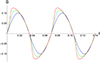Fig. 3. Temporal evolution of initially harmonic non-linear torsional Alfvén waves as a function of the distance from the Sun. The blue line represents the normalized vorticity variation at the base of the solar corona, the green line at a distance of approximately 70 Mm, and the red line at a distance of roughly 140 Mm from the base. The initial wave period is about 50 seconds, and the initial amplitude is 0.1 which corresponds to the initial azimuthal velocity of 100 km/s. The atmosphere maintains an isothermal condition with a temperature of 1.4 MK. The Alfvén speed near the corona’s base is 1000 km/s.

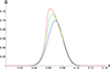Fig. 2. Temporal evolution of initially Gaussian non-linear torsional Alfvén waves as a function of the distance from the Sun. The blue line represents the dimensionless vorticity variation at the base of the solar corona, the green line at a distance of approximately 70 Mm, and the red line at a distance of roughly 140 Mm from the base coronal level. The pulse width is taken about 100 seconds, and the initial amplitude is 0.1 which corresponds to the initial azimuthal velocity of 100 km/s. The atmosphere maintains an isothermal condition with a temperature of 1.4 MK. The Alfvén speed near the corona’s base is 1000 km/s.

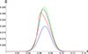Fig. 4. Evolution of an initially Gaussian profile of an Alfvén wave is shown at increasing distances from the Sun, firstly at the base of the corona (depicted by blue line), 1.5 solar radii (the green line), 2.5 solar radii (the black line), and 3.5 solar radii (illustrated by the red line). By considering the impact of the stratification term coefficient in the second term of Eq. (31), the stratified Alfvén speed configuration in Eq. (29), as well as the influence of external pressure denoted by the κ parameter, it becomes evident that the wave’s amplitude gradually decreases with increasing distance from about 1.5 solar radii. At about 3.5 solar radii, the wave experiences a backward shock. The pulse width is taken around 100 seconds and its initial amplitude measures 0.02, which corresponds to the initial azimuthal velocity of 20 km/s. The Alfvén speed near the corona’s base is maintained at 1000 km/s.

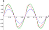Fig. 5. Evolution of an initially harmonic profile of an Alfvén wave is shown at increasing distances from the Sun. Firstly at the base of the corona (depicted by blue line), 1.5 solar radii (the green line), 2.5 solar radii (the black line), and 3.5 solar radii (illustrated by the red line). By considering the impact of the stratification term coefficient in second term of Eq. (31), the stratified Alfvén speed configuration in Eq. (29), as well as the influence of external pressure denoted by the κ parameter, it becomes evident that the wave’s amplitude gradually decreases with increasing distance from about the 1.5 solar radii. At about 3.5 solar radii, the wave experiences a backward shock. The initial wave period is around 50 seconds and its initial amplitude measures 0.02, which corresponds to the initial azimuthal velocity of 20 km/s. The Alfvén speed near the corona’s base is maintained at 1000 km/s.

Figures 6 and 7 illustrate the temporal evolution of initially Gaussian and harmonic non-linear torsional Alfvén wavesm respectively, at a specific distance from the Sun; for instance, about 140 Mm from the coronal base, the vorticity perturbation is visualised for three values of the dimensionless viscosity, $\overline{\nu }$. The selected dimensionless viscosities in increasing order are: $\overline{\nu }=5\times {10}^{-6}$, $\overline{\nu }=5\times {10}^{-5}$, and $\overline{\nu }=5\times {10}^{-4}$. It could be readily noticed that the red curves in both figures, which correspond to the dimensionless viscosity of $\overline{\nu }=5\times {10}^{-4}$ is causing the wave steepening delayed and lowering the wave amplitude, in comparison to the green and blue curves with lower values of the dimensionless viscosity. It can also be noticed from the green and blue curves that although the ratio of the second and first values is equal to the ratio of the second and third values for the viscosity, a jump is observed from the value $\overline{\nu }=5\times {10}^{-5}$ to $\overline{\nu }=5\times {10}^{-4}$; interestingly, this proves that the dissipative effects are not linear. In addition, to demonstrate an quantitative impression; the initial wave period is taken about 50 seconds and the initial amplitude is taken equal to 0.1, which corresponds to the initial azimuthal velocity of 100 km/s. The Alfvén speed near the corona’s base is 1000 km/s.

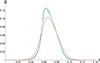Fig. 6. Evolution of an initially Gaussian configuration of an Alfvén wave at a distance of about 140 Mm from the base of the corona is illustrated for three distinct dimensionless viscosities: $\overline{\nu }=5\times {10}^{-6}$ (represented by the blue line), $\overline{\nu }=5\times {10}^{-5}$ (depicted with the green line), and $\overline{\nu }=5\times {10}^{-4}$ (illustrated by the red line). Given the small distinction between the first two diagrams, the green line approximately overlaps with the blue line. The pulse width is taken about 100 seconds, and the initial amplitude is 0.1 which corresponds to the initial azimuthal velocity of 100 km/s. The Alfvén speed near the corona’s base is 1000 km/s.

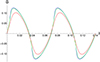Fig. 7. Evolution of an initially harmonic configuration of an Alfvén wave at a distance of about 140 Mm from the base of the corona is illustrated for three distinct dimensionless viscosities: $\overline{\nu }=5\times {10}^{-6}$ (represented by the blue line), $\overline{\nu }=5\times {10}^{-5}$ (depicted with the green line), and $\overline{\nu }=5\times {10}^{-4}$ (illustrated by the red line). Given the small distinction between the first two diagrams, the green line roughly overlaps with the blue line. The initial wave period is about 50 seconds, and the initial amplitude is 0.1 which corresponds to the initial azimuthal velocity of 100 km/s. The Alfvén speed near the corona’s base is 1000 km/s.

Once the interplay of the internal effects (i.e. the parallel structuring and viscous damping against non-linear amplification) is understood, the transverse structuring effects, interestingly packaged in the term κ of Eq. (31), need to be highlighted. Hence, as for the four previous figures, the Gaussian and harmonic profiles for the vorticity (the signature of the character of the Alfvén wave) are visualised in Figs. 4 and 5. The temporal evolution of the pulses are presented while propagating up in the solar atmosphere. It can be readily noticed from both Figs. 4 and 5 that, as the wave propagates from the base of the corona (illustrated by blue curves) to 1.5 solar radii (depicted by green curves), the wave experiences amplification, showing that the stratification and non-linear effects are more pronounced than the damping effects connected with resistivity (as for the ideal conditions illustrated in Figs. 2 and 3). However, as the wave propagates to higher altitudes namely 2.5 solar radii, represented by the black curve, the wave starts to damp. This shows that the increase of the plasma-β external to the plume with altitude in the solar corona (Gary 2001) is making the external medium more effective against the non-linear wave steepening. The result is declining wave amplitude towards 3.5 solar radii presented by red curve. We note that the contribution of the stratification term is due to the second term of Eq. (31), while the stratified Alfvén speed configuration is extracted from Eq. (29), where the influence of external pressure is due to the parameter κ. Interestingly, it is observed that the pulses experience a backward shock while propagating towards higher external plasma-β regions. In all curves the initial wave period is around 50 seconds and its initial amplitude measures 0.02, which corresponds to the initial azimuthal velocity of 20 km/s. The Alfvén speed near the corona’s base is maintained at 1000 km/s.

6. Conclusions

The interaction of MHD waves, especially Alfvén waves, with active region plasmas is an interesting feature of solar physics, especially when it comes to coronal heating. Polar plumes are estimated to have 20 percent contribution towards the solar wind acceleration. Nonetheless, their roles depend on the various stages of their evolution (Zangrilli & Giordano 2020). It is suggested that plumes root in strong unipolar photospheric flux patches. Understanding the wave dynamics in coronal plumes would shed light on their contribution towards solar outflows and energy transfer (Cho et al. 2023). The dense structure of coronal plumes in comparison to their surroundings requires studying transverse structuring in addition to parallel structuring. As the energy transfer has been the main interest of the present study, light has been shed on the dissipative effects connected with coronal plumes. As such, plumes host MHD wave damping even in the non-linear regime where waves tend to steepen. This interplay has been the focus of this study.

In this investigation, we delved into the evolution of torsional Alfvén waves in the solar corona, considering atmospheric stratification and shear viscosity. We also explored the influence of external pressure, linked to a matching coefficient that varies with the parameter plasma-β, on the flux tube, as a boundary effect impacting the propagation of torsional Alfvén waves within the magnetic flux tube. The ensuing results are summarised as follows:

1. We derived an analytical partial differential equation (Eq. (28)) governing the non-linear evolution of torsional Alfvén waves in a funnel waveguide most applicable to a coronal plume, immersed in a uniform plasma medium with magnetic fields parallel to the coronal plume axis. By utilising the second-order thin flux tube approximation, accounting for solar stratification, shear viscosity, and external plasma pressure perturbations a Cohen-Kulsrud-Burgers type evolution equation is presented. Intriguingly, every term of the evolution equation indicates the significance of the actors effective on the induced compressive perturbations due to the Alfvén wave propagation. The second term in Eq. (28) illustrates the evolving impact of stratification with height, while the third term encapsulates the non-linear effects connected with the Alfvén wave and the fourth term is associated with dissipative effects connected with plasma viscosity.

2. For ideal conditions where parallel structuring has small effect and only transverse structuring is present for typical values of the solar corona, the numerical solution of Eq. (31), illustrated in the three curves of Figs. 2 and 3 for both Gaussian and harmonic pulses, the steepening around a height of approximately equal to 140 Mm from the base of the corona is observed. This indicates shock formation.

3. The impact of shear viscosity on non-linear Alfvén waves extracted by Eq. (31) is presented in Figs. 6 and 7, displaying how the amplitude is lowered by the resistivity strength while propagating to higher altitudes expressed by Figs. 4 and 5. The selected dimensionless viscosities in an increasing order proves that the dissipative effects are not linear. Meanwhile, the delay in shock formation enables energy conversion at higher altitudes, thereby maintaining coronal heating at higher levels.

4. The efficiency of parallel structuring and viscous damping is enhanced by the transverse structuring. This is in a sense that their effects become more prominent at higher altitudes where the plasma-β gains finite values above unity (Figs. 4 and 5). On the other hand, for low plasma-β values the shock formation does not really depend on the external medium effects.

5. It is observed that the pulses experience a backward shock while propagating towards higher external plasma-β regions. This is in a sense that the backward shocks appear at around 3.5 solar radii with lower amplitudes, which results in energy transfer at higher altitudes as evident from the comparison between Figs. 2 and 3 with Figs. 4 and 5. The interplay reverses at heights around 1.5 solar radii. From the surface of the sun to the height of 1.5 solar radii, the stratification effect and non-linear dynamics both contribute to amplifying the wave amplitude, acting in concert. However, beyond this threshold, these effects exhibit a reversal of influence in the sense that stratification tends to lower the amplitude of the wave, contrary to the amplifying effect of non-linear dynamics. As depicted in Figs. 4 and 5, the attenuation of amplitude due to stratification post-threshold is more pronounced than the amplification effect of non-linear dynamics.

6. Dissipation scenarios based on Alfvén wave shocks in the solar chromosphere are estimated to provide five percent temperature enhancement (Grant et al. 2018). The findings of the present study support the existence of energy-dissipating mechanisms, such as shock waves, and their key role in heating the plasma and, consequently, hindering the observation of expected oscillations at various atmospheric levels. Hence, the efficiency of Alfvén shock waves in the context of corona heating is highlighted in this work.

In summary, our investigation provides valuable insights into the complex interplay of atmospheric stratification, shear viscosity, and external pressure on the dynamics of torsional Alfvén waves in non-linear regimes of the solar atmosphere. The presented results prove adequate for the dependence of energy conversion due to Alfvén waves on various aspects of the solar atmosphere emphasising on solar shocks. This indicates that coronal heating is maintained at various altitudes due to the interplay of dissipative and amplification processes. The results also prove that the efficiency of each actor regarding wave dynamics may have different outcomes on a specific observable, which may be weakened by the strength of an actor acting against its purported nature.

References

All Figures

Fig. 1. Vertical profiles of the equilibrium properties of a waveguiding magnetic flux tube based on the stratified density and magnetic field intensity models described by Eqs. (15) and (16). (a) Stratified Alfvén speed (CA(z)) inside the flux tube (Eq. (19)) with maximum at around 1.5 solar radii. (b) Stratified tube speed inside the flux tube $(C_{{}_T}(z)\equiv \frac{C_A^2{C}_s^2}{C_A^2+C_s^2})$. (c) Profile of the normalized equilibrium cross-section of the flux tube (Eq. (17)) relative to the tube cross-section at the base of the corona $\left(\frac{A_0(z)}{A_0(0)}\right)$, as a function of height which is normalized by the radius of the sun. The Alfvén speed near the corona’s base is 1000 km/s.

In the text

Fig. 3. Temporal evolution of initially harmonic non-linear torsional Alfvén waves as a function of the distance from the Sun. The blue line represents the normalized vorticity variation at the base of the solar corona, the green line at a distance of approximately 70 Mm, and the red line at a distance of roughly 140 Mm from the base. The initial wave period is about 50 seconds, and the initial amplitude is 0.1 which corresponds to the initial azimuthal velocity of 100 km/s. The atmosphere maintains an isothermal condition with a temperature of 1.4 MK. The Alfvén speed near the corona’s base is 1000 km/s.

In the text

Fig. 2. Temporal evolution of initially Gaussian non-linear torsional Alfvén waves as a function of the distance from the Sun. The blue line represents the dimensionless vorticity variation at the base of the solar corona, the green line at a distance of approximately 70 Mm, and the red line at a distance of roughly 140 Mm from the base coronal level. The pulse width is taken about 100 seconds, and the initial amplitude is 0.1 which corresponds to the initial azimuthal velocity of 100 km/s. The atmosphere maintains an isothermal condition with a temperature of 1.4 MK. The Alfvén speed near the corona’s base is 1000 km/s.

In the text

Fig. 4. Evolution of an initially Gaussian profile of an Alfvén wave is shown at increasing distances from the Sun, firstly at the base of the corona (depicted by blue line), 1.5 solar radii (the green line), 2.5 solar radii (the black line), and 3.5 solar radii (illustrated by the red line). By considering the impact of the stratification term coefficient in the second term of Eq. (31), the stratified Alfvén speed configuration in Eq. (29), as well as the influence of external pressure denoted by the κ parameter, it becomes evident that the wave’s amplitude gradually decreases with increasing distance from about 1.5 solar radii. At about 3.5 solar radii, the wave experiences a backward shock. The pulse width is taken around 100 seconds and its initial amplitude measures 0.02, which corresponds to the initial azimuthal velocity of 20 km/s. The Alfvén speed near the corona’s base is maintained at 1000 km/s.

In the text

Fig. 5. Evolution of an initially harmonic profile of an Alfvén wave is shown at increasing distances from the Sun. Firstly at the base of the corona (depicted by blue line), 1.5 solar radii (the green line), 2.5 solar radii (the black line), and 3.5 solar radii (illustrated by the red line). By considering the impact of the stratification term coefficient in second term of Eq. (31), the stratified Alfvén speed configuration in Eq. (29), as well as the influence of external pressure denoted by the κ parameter, it becomes evident that the wave’s amplitude gradually decreases with increasing distance from about the 1.5 solar radii. At about 3.5 solar radii, the wave experiences a backward shock. The initial wave period is around 50 seconds and its initial amplitude measures 0.02, which corresponds to the initial azimuthal velocity of 20 km/s. The Alfvén speed near the corona’s base is maintained at 1000 km/s.

In the text

Fig. 6. Evolution of an initially Gaussian configuration of an Alfvén wave at a distance of about 140 Mm from the base of the corona is illustrated for three distinct dimensionless viscosities: $\overline{\nu }=5\times {10}^{-6}$ (represented by the blue line), $\overline{\nu }=5\times {10}^{-5}$ (depicted with the green line), and $\overline{\nu }=5\times {10}^{-4}$ (illustrated by the red line). Given the small distinction between the first two diagrams, the green line approximately overlaps with the blue line. The pulse width is taken about 100 seconds, and the initial amplitude is 0.1 which corresponds to the initial azimuthal velocity of 100 km/s. The Alfvén speed near the corona’s base is 1000 km/s.

In the text

Fig. 7. Evolution of an initially harmonic configuration of an Alfvén wave at a distance of about 140 Mm from the base of the corona is illustrated for three distinct dimensionless viscosities: $\overline{\nu }=5\times {10}^{-6}$ (represented by the blue line), $\overline{\nu }=5\times {10}^{-5}$ (depicted with the green line), and $\overline{\nu }=5\times {10}^{-4}$ (illustrated by the red line). Given the small distinction between the first two diagrams, the green line roughly overlaps with the blue line. The initial wave period is about 50 seconds, and the initial amplitude is 0.1 which corresponds to the initial azimuthal velocity of 100 km/s. The Alfvén speed near the corona’s base is 1000 km/s.

In the text

References

- Arregui, I., Kolotkov, D. Y., & Nakariakov, V. M. 2023, A&A, 677, A23 [NASA ADS] [CrossRef] [EDP Sciences] [Google Scholar]
- Banerjee, D., Pérez-Suárez, D., & Doyle, J. G. 2009, A&A, 501, L15 [NASA ADS] [CrossRef] [EDP Sciences] [Google Scholar]
- Bemporad, A., & Abbo, L. 2012, ApJ, 751, 110 [NASA ADS] [CrossRef] [Google Scholar]
- Boocock, C., & Tsiklauri, D. 2022, MNRAS, 510, 1910 [Google Scholar]
- Cho, K.-S., Kumar, P., Cho, I.-H., et al. 2023, ApJ, 953, 69 [CrossRef] [Google Scholar]
- Cranmer, S. R. 2009, Liv. Rev. Sol. Phys., 6, 3 [Google Scholar]
- Duckenfield, T. J., Kolotkov, D. Y., & Nakariakov, V. M. 2021, A&A, 646, A155 [EDP Sciences] [Google Scholar]
- Edwin, P. M., & Roberts, B. 1983, Sol. Phys., 88, 179 [Google Scholar]
- Farahani, S. V., Hejazi, S. M., & Boroomand, M. R. 2021, ApJ, 906, 70 [NASA ADS] [CrossRef] [Google Scholar]
- Gary, G. A. 2001, Sol. Phys., 203, 71 [Google Scholar]
- Ghoraba, A. M., & Farahani, S. V. 2018, ApJ, 869, 93 [NASA ADS] [CrossRef] [Google Scholar]
- Goddard, C. R., Nisticò, G., Nakariakov, V. M., & Zimovets, I. V. 2016, A&A, 585, A137 [NASA ADS] [CrossRef] [EDP Sciences] [Google Scholar]
- Goossens, M. 2003, Astrophysics and Space Science Library (Dordrecht: Kluwer Academic Publishers) [CrossRef] [Google Scholar]
- Goossens, M., Hollweg, J. V., & Sakurai, T. 1992, Sol. Phys., 138, 233 [Google Scholar]
- Grant, S. D. T., Jess, D. B., Zaqarashvili, T. V., et al. 2018, Nat. Phys., 14, 480 [Google Scholar]
- Gruszecki, M., Vasheghani Farahani, S., Nakariakov, V. M., & Arber, T. D. 2011, A&A, 531, A63 [NASA ADS] [CrossRef] [EDP Sciences] [Google Scholar]
- Hahn, M., Landi, E., & Savin, D. W. 2012, ApJ, 753, 36 [NASA ADS] [CrossRef] [Google Scholar]
- Houston, S. J., Jess, D. B., Keppens, R., et al. 2020, ApJ, 892, 49 [NASA ADS] [CrossRef] [Google Scholar]
- Kohutova, P., Verwichte, E., & Froment, C. 2020, A&A, 633, 5 [Google Scholar]
- Krishna Prasad, S., Banerjee, D., & Singh, J. 2012, Sol. Phys., 281, 67 [NASA ADS] [Google Scholar]
- Mandal, S., Yuan, D., Fang, X., et al. 2016, ApJ, 828, 72 [NASA ADS] [CrossRef] [Google Scholar]
- Mandal, S., Krishna Prasad, S., & Banerjee, D. 2018, ApJ, 853, 134 [NASA ADS] [CrossRef] [Google Scholar]
- Mandal, S., Chitta, L. P., Antolin, P., et al. 2022, A&A, 666, L2 [NASA ADS] [CrossRef] [EDP Sciences] [Google Scholar]
- McMurdo, M., Ballai, I., Verth, G., Alharbi, A., & Fedun, V. 2023, ApJ, 958, 81 [NASA ADS] [CrossRef] [Google Scholar]
- Mendoza-Briceño, C. A., Erdélyi, R., & Sigalotti, L. D. G. 2004, ApJ, 605, 493 [CrossRef] [Google Scholar]
- Mozafari Ghoraba, A., Abedi, A., Vasheghani Farahani, S., & Khorashadizadeh, S. M. 2018, A&A, 618, A82 [NASA ADS] [CrossRef] [EDP Sciences] [Google Scholar]
- Nakariakov, V. M. 2004, ASP Conf. Ser., 325, 253 [NASA ADS] [Google Scholar]
- Nakariakov, V. M., Ofman, L., Deluca, E. E., Roberts, B., & Davila, J. M. 1999, Science, 285, 862 [Google Scholar]
- Nakariakov, V. M., Ofman, L., & Arber, T. D. 2000, A&A, 353, 741 [NASA ADS] [Google Scholar]
- Ofman, L., & Davila, J. M. 1995, J. Geophys. Res., 100, 23413 [NASA ADS] [CrossRef] [Google Scholar]
- Ofman, L., Nakariakov, V. M., & Sehgal, N. 2000, ApJ, 533, 1071 [NASA ADS] [CrossRef] [Google Scholar]
- Pant, V., Tiwari, A., Yuan, D., & Banerjee, D. 2017, ApJ, 847, L5 [NASA ADS] [CrossRef] [Google Scholar]
- Petrova, E., Van Doorsselaere, T., Berghmans, D., et al. 2024, A&A, 687, 13 [Google Scholar]
- Pourjavadi, H., Farahani, S. V., & Fazel, Z. 2021, ApJ, 918, 77 [NASA ADS] [CrossRef] [Google Scholar]
- Riedl, J. M., Gilchrist-Millar, C. A., Van Doorsselaere, T., Jess, D. B., & Grant, S. D. T. 2021, A&A, 648, A77 [NASA ADS] [CrossRef] [EDP Sciences] [Google Scholar]
- Ruderman, M. S., & Roberts, B. 2002, ApJ, 577, 475 [Google Scholar]
- Ruderman, M. S., & Petrukhin, N. S. 2018, A&A, 620, A44 [NASA ADS] [CrossRef] [EDP Sciences] [Google Scholar]
- Ruderman, M. S., & Petrukhin, N. S. 2021, MNRAS, 501, 3017 [NASA ADS] [Google Scholar]
- Ruderman, M. S., Nakariakov, V. M., & Roberts, B. 1998, A&A, 338, 1118 [NASA ADS] [Google Scholar]
- Shestov, S. V., Nakariakov, V. M., Ulyanov, A. S., Reva, A. A., & Kuzin, S. V. 2017, ApJ, 840, 64 [Google Scholar]
- Stepanov, A. V., Zaitsev, V. V., & Nakariakov, V. M. 2012, Phys. Usp., 55, 929 [CrossRef] [Google Scholar]
- Terradas, J., Oliver, R., & Ballester, J. L. 2006, ApJ, 650, L91 [NASA ADS] [CrossRef] [Google Scholar]
- Thurgood, J. O., Morton, R. J., & McLaughlin, J. A. 2014, ApJ, 790, L2 [Google Scholar]
- Van Doorsselaere, T., Nakariakov, V. M., & Verwichte, E. 2008, ApJ, 676, L73 [Google Scholar]
- Vasheghani Farahani, S., & Hejazi, S. M. 2017, ApJ, 844, 148 [CrossRef] [Google Scholar]
- Vasheghani Farahani, S., Van Doorsselaere, T., Verwichte, E., & Nakariakov, V. M. 2009, A&A, 498, L29 [NASA ADS] [CrossRef] [EDP Sciences] [Google Scholar]
- Vasheghani Farahani, S., Nakariakov, V. M., & van Doorsselaere, T. 2010, A&A, 517, A29 [NASA ADS] [CrossRef] [EDP Sciences] [Google Scholar]
- Vasheghani Farahani, S., Nakariakov, V. M., Van Doorsselaere, T., & Verwichte, E. 2011, A&A, 526, A80 [NASA ADS] [CrossRef] [EDP Sciences] [Google Scholar]
- Vasheghani Farahani, S., Nakariakov, V. M., Verwichte, E., & Van Doorsselaere, T. 2012, A&A, 544, A127 [NASA ADS] [CrossRef] [EDP Sciences] [Google Scholar]
- Vasheghani Farahani, S., Ghanbari, E., Ghaffari, G., & Safari, H. 2017, A&A, 599, A19 [NASA ADS] [CrossRef] [EDP Sciences] [Google Scholar]
- Wang, T. J., Ofman, L., & Davila, J. M. 2009, ApJ, 696, 1448 [NASA ADS] [CrossRef] [Google Scholar]
- Zangrilli, L., & Giordano, S. M. 2020, A&A, 643, A104 [NASA ADS] [CrossRef] [EDP Sciences] [Google Scholar]
- Zaqarashvili, T. V. 2003, A&A, 399, L15 [CrossRef] [EDP Sciences] [Google Scholar]
- Zaqarashvili, T. V., & Murawski, K. 2007, A&A, 470, 353 [NASA ADS] [CrossRef] [EDP Sciences] [Google Scholar]
- Zhugzhda, Y. D. 1996, Phys. Plasmas, 3, 10 [Google Scholar]
- Zhugzhda, Y. D., & Nakariakov, V. M. 1999, Phys. Lett. A, 252, 222 [NASA ADS] [CrossRef] [Google Scholar]