| Issue |
A&A
Volume 690, October 2024
|
|
|---|---|---|
| Article Number | A167 | |
| Number of page(s) | 12 | |
| Section | Galactic structure, stellar clusters and populations | |
| DOI | https://doi.org/10.1051/0004-6361/202450059 | |
| Published online | 08 October 2024 | |
A detailed study of the very high-energy Crab pulsar emission with the LST-1
1
Department of Physics, Tokai University, 4-1-1, Kita-Kaname, Hiratsuka, Kanagawa 259-1292, Japan
2
Institute for Cosmic Ray Research, University of Tokyo, 5-1-5, Kashiwa-no-ha, Kashiwa, Chiba 277-8582, Japan
3
INFN and Università degli Studi di Siena, Dipartimento di ScienzeFisiche, della Terra e dell’Ambiente (DSFTA), Sezione di Fisica, Via Roma 56, 53100 Siena, Italy
4
Université Paris-Saclay, Université Paris Cité, CEA, CNRS, AIM, F-91191 Gif-sur-Yvette Cedex, France
5
FSLAC IRL 2009, CNRS/IAC, La Laguna, Tenerife, Spain
6
Departament de Física Quàntica i Astrofísica, Institut de Ciències del Cosmos, Universitat de Barcelona, IEEC-UB, Martí i Franquès, 1, 08028 Barcelona, Spain
7
Instituto de Astrofísica de Andalucía-CSIC, Glorieta de la Astronomía s/n, 18008 Granada, Spain
8
IPARCOS-UCM, Instituto de Física de Partículas y del Cosmos, and EMFTEL Department, Universidad Complutense de Madrid, Plaza de Ciencias, 1. Ciudad Universitaria, 28040 Madrid, Spain
9
INAF - Osservatorio Astronomico di Roma, Via di Frascati 33, 00040 Monteporzio Catone, Italy
10
INFN Sezione di Napoli, Via Cintia, ed. G, 80126 Napoli, Italy
11
Max-Planck-Institut für Physik, Föhringer Ring 6, 80805 München, Germany
12
INFN Sezione di Padova and Università degli Studi di Padova, Via Marzolo 8, 35131 Padova, Italy
13
Institut de Fisica d’Altes Energies (IFAE), The Barcelona Institute of Science and Technology, Campus UAB, 08193 Bellaterra (Barcelona), Spain
14
Univ. Savoie Mont Blanc, CNRS, Laboratoire d’Annecy de Physique des Particules - IN2P3, 74000 Annecy, France
15
Universität Hamburg, Institut für Experimentalphysik, Luruper Chaussee 149, 22761 Hamburg, Germany
16
Graduate School of Science, University of Tokyo, 7-3-1 Hongo, Bunkyo-ku, Tokyo 113-0033, Japan
17
Faculty of Science and Technology, Universidad del Azuay, Cuenca, Ecuador
18
INAF - Osservatorio di Astrofisica e Scienza dello spazio di Bologna, Via Piero Gobetti 93/3, 40129 Bologna, Italy
19
Centro Brasileiro de Pesquisas Físicas, Rua Xavier Sigaud 150, RJ, 22290-180 Rio de Janeiro, Brazil
20
Instituto de Astrofísica de Canarias and Departamento de Astrofísica, Universidad de La Laguna, C. Vía Láctea, s/n, 38205 La Laguna, Santa Cruz de Tenerife, Spain
21
CIEMAT, Avda. Complutense 40, 28040 Madrid, Spain
22
INFN Sezione di Bari and Politecnico di Bari, via Orabona 4, 70124 Bari, Italy
23
INAF - Osservatorio Astronomico di Brera, Via Brera 28, 20121 Milano, Italy
24
INFN Sezione di Trieste and Università degli studi di Udine, via delle scienze 206, 33100 Udine, Italy
25
University of Geneva - Département de physique nucléaire et corpusculaire, 24 Quai Ernest Ansernet, 1211 Genève 4, Switzerland
26
INFN Sezione di Catania, Via S. Sofia 64, 95123 Catania, Italy
27
INAF - Istituto di Astrofisica e Planetologia Spaziali (IAPS), Via del Fosso del Cavaliere 100, 00133 Roma, Italy
28
Aix Marseille Univ, CNRS/IN2P3 CPPM, Marseille, France
29
University of Alcalá UAH, Departamento de Physics and Mathematics, Pza. San Diego, 28801 Alcalá de Henares, Madrid, Spain
30
INFN Sezione di Bari and Università di Bari, via Orabona 4, 70126 Bari, Italy
31
INFN Sezione di Torino, Via P. Giuria 1, 10125 Torino, Italy
32
Palacky University Olomouc, Faculty of Science, 17. listopadu 1192/12, 771 46 Olomouc, Czech Republic
33
Dipartimento di Fisica e Chimica “E. Segrè”, Università degli Studi di Palermo, Via Archirafi 36, 90123 Palermo, Italy
34
IRFU, CEA, Université, Paris-Saclay, Bât 141, 91191 Gif-sur-Yvette, France
35
Port d’Informació Científica, Edifici D, Carrer de l’Albareda, 08193 Bellaterrra (Cerdanyola del Vallès), Spain
36
Department of Physics, TU Dortmund University, Otto-Hahn-Str. 4, 44227 Dortmund, Germany
37
University of Rijeka, Department of Physics, Radmile Matejcic 2, 51000 Rijeka, Croatia
38
Institute for Theoretical Physics and Astrophysics, Universität Würzburg, Campus Hubland Nord, Emil-Fischer-Str. 31, 97074 Wärzburg, Germany
39
Department of Physics and Astronomy, University of Turku, Finland, FI-20014 University of Turku, Finland
40
INFN Sezione di Roma La Sapienza, P.le Aldo Moro, 2 - 00185 Rome, Italy
41
ILANCE, CNRS – University of Tokyo International Research Laboratory, University of Tokyo, 5-1-5 Kashiwa-no-Ha, Kashiwa City, Chiba 277-8582, Japan
42
Physics Program, Graduate School of Advanced Science and Engineering, Hiroshima University, 1-3-1 Kagamiyama, Higashi-Hiroshima City, Hiroshima 739-8526, Japan
43
INFN Sezione di Roma Tor Vergata, Via della Ricerca Scientifica 1, 00133 Rome, Italy
44
Faculty of Physics and Applied Informatics, University of Lodz, ul. Pomorska 149-153, 90-236 Lodz, Poland
45
University of Split, FESB, R. Boškovića 32, 21000 Split, Croatia
46
Department of Physics, Yamagata University, 1-4-12 Kojirakawa-machi, Yamagata-shi 990-8560, Japan
47
Institut für Theoretische Physik, Lehrstuhl IV: Plasma-Astroteilchenphysik, Ruhr-Universität Bochum, Universitätsstraße 150, 44801 Bochum, Germany
48
Sendai College, National Institute of Technology, 4-16-1 Ayashi-Chuo, Aoba-ku, Sendai city, Miyagi 989-3128, Japan
49
Josip Juraj Strossmayer University of Osijek, Department of Physics, Trg Ljudevita Gaja 6, 31000 Osijek, Croatia
50
INFN Dipartimento di Scienze Fisiche e Chimiche - Università degli Studi dell’Aquila and Gran Sasso Science Institute, Via Vetoio 1, Viale Crispi 7, 67100 L’Aquila, Italy
51
Kitashirakawa Oiwakecho, Sakyo Ward, Kyoto 606-8502, Japan
52
FZU - Institute of Physics of the Czech Academy of Sciences, Na Slovance 1999/2, 182 21 Praha 8, Czech Republic
53
Astronomical Institute of the Czech Academy of Sciences, Bocni II, 1401-14100 Prague, Czech Republic
54
Faculty of Science, Ibaraki University, 2 Chome-1-1 Bunkyo, Mito, Ibaraki 310-0056, Japan
55
Faculty of Science and Engineering, Waseda University, 3 Chome-4-1 Okubo, Shinjuku City, Tokyo 169-0072, Japan
56
Institute of Particle and Nuclear Studies, KEK (High Energy Accelerator Research Organization), 1-1 Oho, Tsukuba 305-0801, Japan
57
INFN Sezione di Trieste and Università degli Studi di Trieste, Via Valerio 2 I, 34127 Trieste, Italy
58
Escuela Politécnica Superior de Jaén, Universidad de Jaén, Campus Las Lagunillas s/n, Edif. A3, 23071 Jaén, Spain
59
Saha Institute of Nuclear Physics, Sector 1, AF Block, Bidhan Nagar, Bidhannagar, Kolkata, West Bengal 700064, India
60
Institute for Nuclear Research and Nuclear Energy, Bulgarian Academy of Sciences, 72 boul. Tsarigradsko chaussee, 1784 Sofia, Bulgaria
61
Dipartimento di Fisica e Chimica ‘E. Segrè’ Università degli Studi di Palermo, via delle Scienze, 90128 Palermo, Italy
62
Grupo de Electronica, Universidad Complutense de Madrid, Av. Complutense s/n, 28040 Madrid, Spain
63
Institute of Space Sciences (ICE, CSIC), and Institut d’Estudis Espacials de Catalunya (IEEC), and Institució Catalana de Recerca I Estudis Avançats (ICREA), Campus UAB, Carrer de Can Magrans, s/n, 08193 Bellatera, Spain
64
Hiroshima Astrophysical Science Center, Hiroshima University, 1-3-1 Kagamiyama, Higashi-Hiroshima, Hiroshima 739-8526, Japan
65
School of Allied Health Sciences, Kitasato University, Sagamihara, Kanagawa 228-8555, Japan
66
RIKEN, Institute of Physical and Chemical Research, 2-1 Hirosawa, Wako, Saitama 351-0198, Japan
67
Laboratory for High Energy Physics, École Polytechnique Fédérale, CH-1015 Lausanne, Switzerland
68
Chiba University, 1-33, Yayoicho, Inage-ku, Chiba-shi, Chiba 263-8522, Japan
69
Charles University, Institute of Particle and Nuclear Physics, V Holešiovičkáich 2 180 00 Prague 8, Czech Republic
70
Division of Physics and Astronomy, Graduate School of Science, Kyoto University, Sakyo-ku, Kyoto 606-8502, Japan
71
Institute for Space-Earth Environmental Research, Nagoya University, Chikusa-ku, t Nagoya 464-8601, Japan
72
Kobayashi-Maskawa Institute (KMI) for the Origin of Particles and the Universe, Nagoya University, Chikusa-ku, Nagoya 464-8602, Japan
73
Graduate School of Technology, Industrial and Social Sciences, Tokushima University, 2-1 Minamijosanjima, Tokushima 770-8506, Japan
74
INFN Sezione di Pisa, Edificio C – Polo Fibonacci, Largo Bruno Pontecorvo 3, 56127 Pisa, Italy
75
Dipartimento di Fisica - Università degli Studi di Torino, Via Pietro Giuria, 1 - 10125 Torino, Italy
76
INFN Dipartimento di Scienze Fisiche e Chimiche - Università degli Studi dell’Aquila and Gran Sasso Science Institute, Via Vetoio 1, Viale Crispi 7, 67100 L’Aquila, Italy
77
Gifu University, Faculty of Engineering, 1-1 Yanagido, Gifu 501-1193, Japan
78
Department of Physical Sciences, Aoyama Gakuin University, Fuchinobe, Sagamihara, Kanagawa 252-5258, Japan
79
Department of Astronomy, University of Geneva, Chemin d’Ecogia 16, CH-1290 Versoix, Switzerland
80
Graduate School of Science and Engineering, Saitama University, 255 Simo-Ohkubo, Sakura-ku, Saitama city, Saitama 338-8570, Japan
81
Department of Physics, Konan University, 8-9-1 Okamoto, Higashinada-ku Kobe 658-8501, Japan
Received:
21
March
2024
Accepted:
28
June
2024
Abstract
Context. To date, three pulsars have been firmly detected by imaging atmospheric Cherenkov telescopes (IACTs). Two of them reached the TeV energy range, challenging models of very high-energy (VHE) emission in pulsars. More precise observations are needed to better characterize pulsar emission at these energies. The LST-1 is the prototype of the large-sized telescopes, which will be part of the Cherenkov Telescope Array Observatory (CTAO). Its improved performance over previous IACTs makes it well suited for studying pulsars.
Aims. In this work we study the Crab pulsar emission with the LST-1, improving upon and complementing the results from other telescopes. Crab pulsar observations can also be used to characterize the potential of the LST-1 to study other pulsars and detect new ones.
Methods. We analyzed a total of ∼103 hours of gamma-ray observations of the Crab pulsar conducted with the LST-1 in the period from September 2020 to January 2023. The observations were carried out at zenith angles of less than 50 degrees. To characterize the Crab pulsar emission over a broader energy range, a new analysis of the Fermi/LAT data, including ∼14 years of observations, was also performed.
Results. The Crab pulsar phaseogram, long-term light curve, and phase-resolved spectra are reconstructed with the LST-1 from 20 GeV to 450 GeV for the first peak and up to 700 GeV for the second peak The pulsed emission is detected with a significance level of 15.2σ. The two characteristic emission peaks of the Crab pulsar are clearly detected (> 10σ), as is the so-called bridge emission between them (5.7σ). We find that both peaks are described well by power laws, with spectral indices of ∼3.44 and ∼3.03, respectively. The joint analysis of Fermi/LAT and LST-1 data shows a good agreement between the two instruments in their overlapping energy range. The detailed results obtained from the first observations of the Crab pulsar with the LST-1 show the potential that CTAO will have to study this type of source.
Key words: astroparticle physics / stars: neutron / pulsars: general / pulsars: individual: Crab pulsar / gamma rays: stars
Corresponding authors; This email address is being protected from spambots. You need JavaScript enabled to view it. .
© The Authors 2024
 Open Access article, published by EDP Sciences, under the terms of the Creative Commons Attribution License (https://creativecommons.org/licenses/by/4.0), which permits unrestricted use, distribution, and reproduction in any medium, provided the original work is properly cited.
This article is published in open access under the Subscribe to Open model. This email address is being protected from spambots. You need JavaScript enabled to view it. to support open access publication.
1. Introduction
Pulsars are highly magnetized and rapidly rotating neutron stars that emit beamed radiation from the radio up to gamma rays. Although almost 300 gamma-ray pulsars have been identified so far with the Fermi/Large Area Telescope (LAT; Smith 2023), only three pulsars have been detected by imaging atmospheric Cherenkov telescopes (IACTs) at a significance level above 5σ: the Crab pulsar (Aliu et al. 2008; López et al. 2009), the Vela pulsar (Abdalla et al. 2018), and the Geminga pulsar (Acciari et al. 2020). Each of these three pulsars is unique. Two of them, Crab and Vela, have been detected at TeV energies (Ansoldi et al. 2016; Aharonian et al. 2023). The emission and pulse profile found at such high energies cannot be easily explained with the curvature radiation models that predict suppression of the emission at a few GeV. In the case of Vela, the TeV emission is associated with a second radiation component that reaches 20 TeV (Aharonian et al. 2023).
Detecting more pulsars at tens of GeV with ground-based gamma-ray telescopes is a challenge due to their faint emission at those energies. Fermi/LAT measurements of gamma-ray pulsars show cutoffs in the spectra at a few GeV (Smith 2023). Due to the low expected fluxes from these sources above 50 GeV (McCann 2015), the current generation of IACTs is not expected to detect more pulsars. The search for more pulsars is necessary to understand whether the very high-energy (VHE; E > 100 GeV) emission of these objects is something unique or if there is a whole population of VHE pulsars. Therefore, improving the sensitivity of IACTs is necessary for studying new gamma-ray pulsars above 10 GeV and constrain the models at those energies.
The Cherenkov Telescope Array Observatory (CTAO; Zanin et al. 2021) will be the next generation of IACTs. It will be located at two sites, one in each hemisphere to cover the full VHE sky. CTAO will be composed of an array of multiple telescopes of different sizes, increasing by over an order of magnitude the sensitivity of current IACTs. The large-sized telescopes (LSTs; Cortina 2019) will be the largest ones, with a dish diameter of 23 meters, and will be optimized for low energies (20–200 GeV). The LST-1 is a fully equipped LST prototype built at the Roque de los Muchachos Observatory (ORM) on the island of La Palma (Abe et al. 2023a). It was inaugurated in 2018 and is now producing its first science results after several years of commissioning (Abe et al. 2023b,c).
The Crab pulsar and nebula are the remnants of the supernova 1054 event. Due to its young age, it is a very energetic pulsar (Ė ≈ 4.6 · 1038erg s−1; Lyne et al. 2014) with a rotation period of P ≈ 33 ms (Staelin & Reifenstein 1968). The Crab pulsar was first detected and studied in the radio (Comella et al. 1969), and afterward in almost all wavelengths. The pulsed emission from the Crab pulsar above 25 GeV was first detected by the Major Atmospheric Gamma Imaging Cherenkov (MAGIC) telescopes, ruling out the existence of the super-exponential cutoff predicted by polar cap models (Aliu et al. 2008; Aleksić et al. 2011). This fact was confirmed after the study of the pulsar with Fermi/LAT, which hint at the existence of a sub-exponential cutoff in the spectrum at a few GeV (Abdo et al. 2009a), a feature that was found in other gamma-ray pulsars. The pulsar was detected in the VHE regime up to 400 GeV by MAGIC (Aleksić et al. 2012) and the Very Energetic Radiation Imaging Telescope Array System (VERITAS) (Aliu et al. 2011). A few years later, MAGIC reported the detection of the Crab pulsar up to 1.5 TeV (Ansoldi et al. 2016). The overall emission at VHEs can be described well by a power law (PWL), supporting those models that consider inverse Compton (IC) processes in the outer magnetosphere or beyond.
In this work we describe the analysis and results obtained from the first observations of the Crab pulsar with the LST-1. Our aim is to characterize the emission of the pulsar above 20 GeV with LST-1 and Fermi/LAT data and examine the potential of this new telescope for the study of pulsars at VHEs.
2. LST-1 observation overview
The LST-1 observed the Crab Nebula and pulsar during the first years of operation as part of its commissioning program. A total of more than 150 hours were collected from September 2020 to January 2023. The data were taken in 20-minute runs in wobble mode (Fomin et al. 1994), where the source is located at a 0.4-degree offset from the camera center. We applied quality cuts to the data, removing those runs with low trigger and pixel rates (see more details in Abe et al. 2023b). In addition, we used only data taken in dark conditions. We also discarded those runs affected by technical problems.
As a result, ∼103 hours of observations taken at zenith distance (Zd) below 50 deg survived the quality cuts and were used in the final analysis. Out of these, 76 hours were collected at Zd < 35 deg, half of them below 25 deg, decreasing the overall energy threshold down to ∼20 GeV in the analysis (Abe et al. 2023b). The trigger settings of the telescope were variable before August 2021, so the energy threshold of data taken before that date is less stable and slightly higher than that of data collected afterward. The improvements in the telescope threshold are a consequence of the advances made during the commissioning of LST-1.
3. Data analysis
3.1. LST-1 data analysis
LST-1 data were reduced using cta-lstchain v0.9.14 (López-Coto 2022; López-Coto et al. 2023), a software designed for the data analysis of the LST-1, following the usual IACT analysis chain. This allowed us to clean and parametrize the images produced in the camera by atmospheric showers. The image parametrization is used to infer the direction and energy (called reconstructed energy) of the primary particle through trained random forest (RF) algorithms (Albert et al. 2008). An additional parameter called gammaness is computed, defined as a score that rises for the higher resemblance of the event to a gamma-ray initiated one. To optimize the analysis of faint showers (i.e., low-intensity images), we included in the training some parameters that depend on the known position of the source in the camera plane in the so-called source-dependent approach. This improves the performance with respect to the standard source-independent analysis (see Sect. 4.1.4). One of the source-dependent parameters added is alpha, defined as the angle between the major axis of the fitted shower ellipse and the line that joins the center of gravity of the image and the assumed source position in the camera plane.
We used Monte Carlo (MC) simulations to evaluate the performance of the telescope. The MC simulations of gamma-ray-initiated showers used in this work are part of an all-sky MC production simulated in declination lines (Abe et al. 2023b). The one used to analyze the data sample is the closest to that of the Crab pulsar (22.76 deg). The MC data were tuned by adding Poissonian noise to match the real night sky background of the Crab pulsar region. The MC sample was processed with the help of the lstmcpipe package (Garcia et al. 2022; Vuillaume et al. 2022). Two samples were produced: a sample to train the RF, and a test sample to characterize the response of the telescope. The MC test dataset was simulated on a grid of nodes with different zenith/azimuth pointings in the sky. To calculate the instrument response functions (IRFs), we used the nodes closest to the pointing of the telescope during the observations. This way, it is possible to account for the dependence of the telescope performance on the airmass and the angle formed by the orthogonal component of the geomagnetic field and the pointing of the telescope.
After the reconstruction of the events, several cuts were applied. First, an intensity cut is needed to provide a common analysis threshold for the entire data sample and a good match between observed data and MC, as explained in Abe et al. (2023b). We applied an overall intensity cut of 80 photoelectrons (p.e.) to all the data taken before August 2021, and an intensity cut of 50 p.e. to the data taken after that date to account for the different trigger thresholds of the telescope during these periods (see Sect. 2). In addition, we applied energy-dependent cuts on the direction (alpha) and gammaness, computed by setting a 70% MC efficiency on the gamma MC sample for each of the cuts separately.
The last step in analyzing the pulsar is to obtain the phase of the rotation of the star associated with each event. For that, we used the PINT package v0.9.3 (Luo et al. 2021) and the Crab pulsar ephemeris provided by the Jodrell Bank Observatory (Lyne et al. 1993)1. Finally, the spectral results of the analysis were produced with Gammapy v1.0.1 (Donath et al. 2023; Acero et al. 2023). As a consistency check for the analysis, we compared (a posteriori) the weighted distributions of the MC shower parameters with those of the pulsed excess, finding a good agreement.
As in any measurement, there will be systematic uncertainties in the results shown in this paper, for instance, due to the mismatch between MC simulations and real data or biases in the estimation of the real energy of the events. This may also cause a relative error in the energy scale between Fermi and LST-1 that must be evaluated and will be discussed in the corresponding sections.
The Crab pulsar is characterized by showing two emission peaks in each rotation, which remain aligned at all wavelengths. The first peak, located at phase 0, is defined as P1 and is the most intense in the radio and also in the Fermi/LAT sample between 100 MeV and 1 GeV. The second peak, P2, is however the most intense at VHEs. For the analysis, we adopted the phase intervals defined in Aleksić et al. (2012), namely P1 = [–0.017, 0.026] and P2 = [0.377, 0.422]. The background level was estimated using the OFF region [0.52, 0.87], where no pulsed emission is expected.
3.2. Fermi/LAT data analysis
Since its launch in 2008, Fermi/LAT has been observing the gamma-ray sky continuously in the energy range between 20 MeV to hundreds of GeV. To study the Crab pulsar emission at energies lower than those accessible to the LST-1, we analyzed public Fermi/LAT data taken from August 4, 2008, until August 24, 2022. This resulted in ∼14 years of observations, extending the sample used in previous works (Yeung 2020).
We processed this dataset using the Fermi Science Tools version v11r5p3 (Fermi Science Support Development Team 2019) and the P8R2_SOURCE_V6 IRFs. We selected events classified as event class 128 (“Source”) and event type 3 from a circular region of interest (ROI) of 15 deg centered at the Crab pulsar coordinates, RA = 05h34m31.9s, Dec = 22 ° 00′52.2″. To reject the background coming from the Earth’s limb, we excluded time intervals where the ROI was observed at zenith angles greater than 90 deg. The pulsar rotational phases were computed using the Tempo2 package (Hobbs et al. 2006) with the same ephemeris as for the LST-1 data analysis. The consistency between Tempo2 and PINT is proved in Luo et al. (2021). We also verified it by comparing the phases obtained by the two pieces of software for a single run, finding a maximum error of 10−7. Phase-filtered event files were produced, containing only photons in the OFF phase region, or in the phase region corresponding to each of the pulsar emission peaks defined above.
For the spectral reconstruction, we performed a binned likelihood analysis using the pyLikelihood python module of the Fermi Science Tools, with a bin size of 0.2° per pixel and 40 logarithmically spaced energy bins between 100 MeV and 2 TeV. The initial spectral-spatial model included all sources from the LAT 10-year source catalog (4FGL; Abdollahi et al. 2020) within the ROI that was expanded by 5 deg to account for partially contained sources. The spectral parameters for sources with a significance higher than 5σ and located within 5 deg of the center of the ROI were left free. Also, the normalization factor of the Galactic (gll_iem_v07.fits) and isotropic background (iso_P8R3_SOURCE_V3_v1.txt) models were let free. For the rest of the sources, the spectral parameters were set to their catalog values. After the first fit, all sources with TS < 4 were removed from the model. We then use the events in the OFF region to characterize the gamma-ray background due to emission from the Crab Nebula, whose IC and synchrotron components appear as two different sources in the catalog, J0534.5+2201i and 4FGL J0534.5+2201s, respectively. After this, the Crab Nebula spectral parameters were left fixed, scaling only the normalization factor to account for the different phase widths of the off-pulse and peak regions. Finally, the spectra of P1 and P2 were analyzed independently, using smooth broken PWL models. To obtain the spectral points we repeated the spectral fit in each energy bin using a PWL model with a fixed spectral index of 2 and with the normalization factor free. Only spectral points with a significance higher than 2σ are shown in the plots.
4. Results
4.1. Phaseogram
4.1.1. Pulsed signal
The phase-folded phaseogram obtained with the LST-1 is shown in Fig. 1. P1 and P2 are detected at a statistical significance of 10.5σ and 12.1σ, respectively, computed using formula (17) in Li & Ma (1983). The joint pulsed emission (P1+P2) is detected at 15.2σ. Between the two peaks a fainter signal, commonly known as the bridge emission, is found. In this work, we use the two definitions for the bridge used in Aleksić et al. (2014). Defining the bridge as the whole region between peaks (i.e., BridgeM = [0.026,0.377]) the emission is detected at a significance level of 5.7σ. If we redefine the bridge region as done in Fierro et al. (1998) (BridgeE = [0.14,0.25]) the significance is 3.7σ.
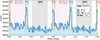 |
Fig. 1. Phaseogram of the Crab pulsar sample from LST-1 data (Zd < 50 deg). Both peaks and the overall bridge emission between peaks are detected significantly. Most of the pulsed signal is provided by data at Zd < 25 degrees, so the energy threshold of the sample is Eth ∼ 20 GeV. The period corresponding to two rotations is shown in the phaseogram for better visualization. |
The increase in the signal with time, as seen in Fig. 2, confirms the stability of the analyzed data sample. We did a fit of the data finding that the evolution can be characterized by σP1(h) = (0.916 ± 0.021)h1/2, σP2(h) = (1.133 ± 0.012)h1/2 and σBridge(h) = (0.478 ± 0.018)h1/2, where h is the total number of hours of observation. These values change if we limit our sample to lower zenith angles. For instance, at Zd < 35 deg, the values increase up to σP1(h) = (1.109 ± 0.016)h1/2, σP2(h) = (1.272 ± 0.014)h1/2 and σBridge(h) = (0.619 ± 0.017)h1/2. These results highlight the good performance of the LST-1. For comparison, the stereo MAGIC SumTrigger-II reported an overall detection rate of σP1 + P2 = 2.0h1/2 for the Crab pulsar at Zd < 25 deg (Ceribella et al. 2019), similar to the detection rate of a single LST-1 telescope (σP1 + P2 ≈ 1.8h1/2) at the same zenith.
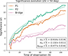 |
Fig. 2. Evolution of the significance with the total time of observation for P1, P2, and the bridge emission, defined as BridgeM = [0.026,0.377]. |
4.1.2. Morphology of the peaks
The phaseogram was also studied in different energy bins. In particular, we divided our sample into seven bins from 20 GeV to 700 GeV (see Fig. 3), approximately 5 bins per decade. The upper edge was chosen to include the last bin where a hint of signal for P2 (> 1.5σ) is found. Assuming that the peaks follow symmetric Gaussian distributions, we fitted the phaseogram to a double Gaussian model (i.e., two Gaussians joint together) with an overall background to study the morphology of the peaks. Since P1 and P2 were fitted together, the same number of points were obtained for both peaks. The bridge contribution was neglected in the fits since it is not significant above 100 GeV. Making that assumption could introduce an additional error in the first two bins, but the strong signal from both peaks compared to the bridge assures that this error is low. The values of the mean phase and width of each peak are shown in Table 1. To assess the goodness of the fit, we computed the χ2/ndf of each fit, all of which were close to 1. The peak positions do not shift significantly. The width of P2 seems to decrease with energy (see Fig. 4). This feature, which crucial to understanding emission models at energies greater than 100 GeV (Harding et al. 2021), was already found in other studies (Aleksić et al. 2012). The LST-1 measurement in Fig. 4 was fitted to a linear model (FWHM = m ⋅ log(E)+n) above 20 GeV, finding that for P2 the best fit has a slope of mP2 = 0.041 ± 0.009 and shows a pvalue = 0.65. For P1 the fitted model to the LST-1 data shows a slope of mP1 = 0.016 ± 0.013. Although for this model pvalue = 0.31, the large statistical uncertainties of the LST-1 points make it difficult to conclude a significant variation of the width of P1 above 20 GeV.
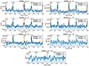 |
Fig. 3. Phaseogram of the Crab pulsar from LST-1 data in different energy bins from 20 GeV to 700 GeV. The statistical significance of each peak is given in each plot. The black line shows the best fits to the pulse profile. Above 250 GeV the fit was not successful since the signal of P1 begins to disappear. |
Peak position (μ) and width (FWHM) of each peak, P1 and P2.
The Fermi/LAT data were also divided into energy bins and the phaseogram was fitted to the same model as for the LST-1 data. Representing the width of the peaks as a function of energy from MeV to GeV (Fig. 4) one can see a soft transition between Fermi/LAT and LST-1 data. For both peaks, the width above 20 GeV is lower than at 200 MeV as seen in other works (Aliu et al. 2011; Aleksić et al. 2012). Since the energy reconstruction is different for the two instruments, a systematic error exists (see Sect. 3.1), although a direct quantification of them is difficult due to a lack of theoretical prediction for the full width at half maximum (FWHM) of the peaks. However, Fermi/LAT and LST-1 results in Fig. 3 are compatible in their overlapping energy region for P2. For P1, the FWHM points of both instruments are at a similar level and to make them fully compatible we would only need to add a < ∼20% systematic error between the two instruments.
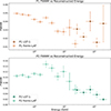 |
Fig. 4. Evolution of the peak width as a function of the energy from 100 MeV to 200 GeV using Fermi/LAT and LST-1 data. The fit of the LST-1 data was not successful above 200 GeV due to the lack of statistics. |
4.1.3. P1/P2 ratio
As seen in Fig. 3, the intensity and significance of P1 is higher in the lowest-energy bin, below 30 GeV. In the rest of the bins, P2 appears stronger than P1. To study this trend, the LST-1 differential ratio of P1/P2 was determined as well from the excess counts in each reconstructed energy bin. The same ratio was computed with the Fermi/LAT sample in 13 energy bins to plot the energy evolution of the differential ratio. As a result, we covered the energy range from 100 MeV up to 400 GeV using both instruments. The result is depicted in Fig. 5. One can see a fast decrease in the ratio from MeV down to ∼0.5 at ∼200 GeV. This trend was already found in other works (Aliu et al. 2011; Aleksić et al. 2012; Mirzoyan et al. 2022). The P1/P2 ratio achieves 1 at Eeq ≈ 30 GeV. The overall LST-1 ratio, integrated over the entire energy range, is P1/P2 = 0.84 ± 0.11. The LST-1 points show lower statistical errors than the Fermi/LAT ones, indicating that the LST-1 can provide more accurate results above 20 GeV even with only 100 hours.
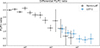 |
Fig. 5. Evolution of the P1/P2 ratio as a function of the energy from 100 MeV to 400 GeV using Fermi/LAT and LST-1 data. The fit of the LST-1 data was not successful above 400 GeV due to the lack of statistics for P1. |
The P1/P2 ratio points of LST-1 derived in Fig. 5 are represented in reconstructed energy. Near the threshold of the LST-1 the reconstructed energy of the events is systematically greater than the true one. This introduces a systematic error, as mentioned in Sect. 3.1. The maximum systematic error in the differential P1/P2 computation at low energies due to the energy dispersion of our system is ∼20% as estimated from a set of MC simulations with a similar zenith distribution as our data. For the integral ratio, the maximum of this systematic error drops to ∼12%. Thus, the LST-1 P1/P2 ratios in each reconstructed energy container are therefore overestimated with respect to those of Fermi/LAT by at most that 20%.
4.1.4. Source-dependent versus source-independent
Apart from the source-dependent phaseogram shown in Fig. 1, a source-independent one (i.e., excluding source-dependent parameters in the RF training) was computed to compare the performance of the two methods. The analysis chain was similar to the one used for the source-dependent case but changing the MC efficiency to 91% to have a similar background rate in the two approaches. In particular, for this efficiency, we get a difference in background level < 1%. The results are shown in Table 2. The source-dependent analysis shows better performance for studying the pulsed emission, with a difference of 1.5σ in P1 and 2.7σ in P2.
Comparison of the pulsed signal using source-dependent and source-independent approaches in the RF training.
The results described in Abe et al. (2023b) show that the sensitivity curves below 100 GeV are similar for both source-dependent and source-independent analysis. The difference found in the Crab pulsar analysis indicates that the source-dependent approach improves the sensitivity at the lowest true energies, near the threshold of the telescope, where the signal of the pulsar is more intense and the background estimation in the Crab Nebula is more uncertain.
4.2. Long-term light curve
In order to test for possible variability in the Crab pulsar flux, we computed the long-term light curve of the pulsed emission for both P1 and P2 above 30 GeV. The minimum energy was selected to minimize the effect of energy migration near the telescope threshold for the variability studies. We divided the sample into variable time bins requiring a fixed number of excess events for the total pulsed emission. We selected a value of Nex = 1500 to achieve at least ∼3σ for the entire pulsed emission in each bin. In Fig. 6 the corresponding long-term light curve for each peak is shown.
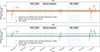 |
Fig. 6. Long-term light curve of P1 and P2 Crab emission above 30 GeV. Each variable time bin contains 1500 excess events in the combined phase regions P1 and P2. This value was chosen to reach at least ∼3σ for the entire pulsed emission (P1+P2) in each bin. The horizontal bars indicate the time range of each bin. The flux was fit to a constant function, shown by the green line. The dashed green area represents the statistical uncertainties of the fitted flux. The reference integrated flux above 30 GeV using the MAGIC+Fermi/LAT SED reported in Ansoldi et al. (2016) is included in gray. The regions where the Crab pulsar was not observable are shown in blue, namely two summer periods and the volcano eruption that took place from September to December 2021 in La Palma. |
We fitted the flux points to a constant function and performed a χ2 test on the data. We found a value of χ2/ndf = 13.1/10 (pvalue = 0.22) and χ2/ndf = 4.7/10 (pvalue = 0.91) for P1 and P2, respectively. For the total pulsed emission, a value of χ2/ndf = 12.8/10 (pvalue = 0.24) is found. Therefore, no hint of flux variability is detected in the sample, and the fluxes are compatible with constant functions of fP1 = (4.4 ± 0.6) ⋅ 10−11 cm−2 s−1 and fP2 = (5.3 ± 0.5) ⋅ 10−11 cm−2 s−1 showing a weighted relative root mean squared error of 46% for P1 and 22% for P2. For comparison, we calculated the integral flux using the joint MAGIC and Fermi/LAT spectral energy distribution (SED) reported in Ansoldi et al. (2016) above 30 GeV. For P1, we obtained a value of fref, P1 = (3.8 ± 0.6) ⋅ 10−11 cm−2 s−1 compatible with the LST-1 integral flux. In the case of P2, we found a value of fref, P2 = (4.0 ± 0.4) ⋅ 10−11 cm−2 s−1, lower than for the LST-1 sample. This could be a result of the different energy thresholds for MAGIC and for the LST-1, also reflected in the distinct spectral fits obtained for both.
4.3. Spectral energy distribution of the peaks
In addition to the phaseogram and long-term light curve, the SED for P1 and P2 is shown in Fig. 7. Both peaks are well described by a PWL model (dϕ/dE = ϕ0(E/E0)−Γ) between 20 GeV and 700 GeV. The fit results are summarized in Table 3. The reference energy E0 was set to the de-correlation energy for each peak, defined as the energy that minimizes the correlation between the normalization flux ϕ0 and the rest of the parameters of the model (see Eq. (1) in Abdo et al. 2009b). The spectral index of P2 (Γ2 = 3.03 ± 0.09) is considerably harder than the one for P1 (Γ1 = 3.44 ± 0.15), while the flux for P1 is slightly larger below 30 GeV. These results are consistent with the most recent results from MAGIC (Ansoldi et al. 2016; Ceribella 2021) and VERITAS (Aliu et al. 2011; Nguyen 2016). Moreover, we confirm the PWL extension of P2 found by MAGIC and VERITAS above 500 GeV.
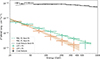 |
Fig. 7. LST-1 SED of P1 and P2 of the Crab pulsar from 20 GeV to 700 GeV. The Crab Nebula spectrum obtained with the same sample is represented in black. |
Fitted parameters of the spectral model, with their statistical uncertainties, for each region.
Pulsar analysis does not suffer from the systematic uncertainties in the background estimation that dominated the study of the Crab Nebula performance (Abe et al. 2023b). Thus, it is possible to quantify additional systematic uncertainties of the telescope with the pulsar signal. We tested different parameters in the analysis such as the cut efficiencies or the zenith angle and intensity cuts. We also shifted the true energy of the MC (up to 10%), and computed the modified IRFs and spectra to test for a possible bias in the energy reconstruction. Additionally, we compared the SED of different subsamples in the analysis. Adding all the contributions, the systematic uncertainties in the reconstruction of the spectral index for P1 and P2 is ∼0.34 and ∼0.21, while the uncertainties in the fluxes rise to ∼45% and ∼20%, respectively. These numbers are compatible with the ones found in the Crab Nebula study with the LST-1 above 60 GeV.
To estimate the analysis energy threshold we used the MC simulations, weighing their spectrum by the one found in the Crab pulsar. These simulations were analyzed using the same analysis chain as for the observations. The peak of the true energy distribution of the MC events gives the energy threshold (Eth) of the analysis, which depends on the Zd. For the LST-1 at Zd = 10 deg, the threshold estimated from the MC energy distribution is Eth = (18 ± 1) GeV, while at Zd = 23 deg it is Eth = (22 ± 1) GeV and at Zd = 32 deg it increases to Eth = (29 ± 2) GeV. We estimate that for a spectrum similar to that of the Crab pulsar, with the same zenith distribution as for the LST-1 observations, the energy threshold below 35 degrees is ≈20 GeV.
4.4. Joint Fermi/LAT and LST-1 SED of the peaks
Precise measurements at tens of GeV, in the energy range overlapping between Fermi/LAT and IACT, are needed to study the existence of spectral cuts or other spectral components. In this work, a joint fit with both LST-1 and Fermi/LAT data was performed between 100 MeV and 450 GeV for P1 and up to 700 GeV for P2. Two models were tested. The first model is a smooth broken PWL (SmoothBPWL, Eq. (1)), and the second one is a typical PWL with a sub-exponential cutoff (ExpCutPWL, Eq. (2)):
 (1)
(1)
 (2)
(2)
Both models were fit using a forward folding algorithm. The results of the fits together with the spectral points for P1 and P2 are shown in Fig. 8 and summarized in Table 4. MAGIC spectral points are also shown for comparison. A smooth transition between the instruments is clear and the spectral points of the LST-1 are compatible with the Fermi/LAT and the MAGIC points. The low statistical uncertainties of the LST-1 spectral points show that the telescope can fill the region between 20 GeV and 50 GeV with higher statistics than previous works from MAGIC (∼60 hours analyzed in Aleksić et al. 2011).
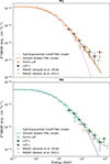 |
Fig. 8. SED and joint fit using Fermi/LAT and LST-1 data from 100 MeV to 700 GeV for both P1 and P2 of the Crab pulsar. The points from MAGIC working in stereo are shown as well. |
Results of the best fits to the LST-1 and Fermi/LAT data for each peak and model.
The goodness of the fit for the two models was compared using two statistics. The first one is the Akaike information criterion (AIC), defined as AIC = 2k − 2log L where k is the number of free parameters and L is the likelihood of the model. The second one is the Bayesian information criterion (BIC) defined as BIC = k lnn − 2log L where n is the size of the sample. Both are information criteria that do not allow us to compute a p-value but to recognize in a qualitative way which model agrees better with the data. The smooth broken PWL shows, in general, a lower AIC and BIC value. For P1 this difference is Δ(AIC)P1 = 8.4 and Δ(BIC)P1 = 7.0; in the case of P2 the differences raise up to Δ(AIC)P2 = 22.0 and Δ(BIC)P2 = 20.6. This points to the smooth broken PWL as the preferred model to describe the observed fluxes. This is also observed in Fig. 8, where although both fits seem to fit well in the low-energy spectrum, the VHE spectral points agree better with the smooth broken PWL.
4.5. SED of the bridge emission
The SED of the Crab pulsar bridge emission for each of the bridge regions defined in Sect. 4.1.1 is shown in Fig. 9. The LST-1 SED was fitted to a PWL between 20 GeV and 200 GeV. The results are shown in Table 3, the spectral indexes are ΓM = (3.5 ± 0.4) and ΓE = (3.3 ± 0.6). The LST-1 flux points are compatible with those reported by the MAGIC collaboration (Aleksić et al. 2014), which extend up to 200 GeV. Above 100 GeV for the LST-1 the significance of the flux points is lower than for MAGIC and only upper limits can be calculated.
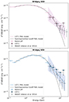 |
Fig. 9. LST-1 SED from 20 GeV to 200 GeV for the two definitions of the bridge emission of the Crab pulsar. The Fermi/LAT + LST-1 joint fit to the sub-exponential cutoff PWL model is shown as a solid line. The points from MAGIC working in stereo are shown as well. |
In addition, we did a joint fit using Fermi/LAT data and LST-1 from 200 MeV to 200 GeV. Data below 200 MeV were excluded from the fit because the analysis at the lowest energies led to unreliable flux estimation as indicated in Fig. 9. In this case, since the signal above 100 GeV drops fast, we could only fit successfully the sub-exponential cutoff PWL model (shown in the solid line in Fig. 9). The results are shown in Table 3. Although there is a hint of a PWL extension for both definitions, the lack of statistics prevents us from confirming or rejecting the existence of a cutoff in the bridge spectra.
5. Discussion and conclusions
In this work we have reported a detailed analysis of the first VHE gamma-ray pulsar detected with the LST-1. The results show that the LST-1 can detect the signal of the Crab pulsar at a high significance level and reconstruct its SED from 20 GeV up to 450 GeV for P1 and 700 GeV for P2. Both P1 and P2 are significantly detected (> 10σ) in this analysis. The VHE gamma-ray SED of each peak is well reproduced by a PWL that is compatible with previous results from the literature. P1 shows a softer spectrum (Γ1 = 3.44 ± 0.15) than P2 (Γ2 = 3.03 ± 0.09). The two peaks show similar fluxes (∼3.5 ⋅ 10−9 cm−2 s−1 TeV−1) at E = 30 GeV. The bridge emission is also significantly detected, and the resulting spectra, for both definitions, are well described by PWLs with spectral indices ΓE = 3.3 ± 0.6 and ΓM = 3.5 ± 0.4 for BridgeE and BridgeM, respectively. We also studied the long-term light curve of the Crab pulsar using the LST-1 data over three different years, finding a value of χ2 = 12.8/10 when the pulsed integral flux is fit to a constant, demonstrating the stability of the overall energy released in the pulsed signal over time within our statistical uncertainties.
The consistency of the LST-1 results in the region overlapping with Fermi/LAT proves its performance at E < 50 GeV. The results are also consistent with those at the higher energies measured by MAGIC. We performed joint Fermi/LAT and LST-1 fits to study the overall gamma-ray emission of the Crab pulsar over four decades of energy. For both P1 and P2, there is a smooth transition in the SED measured by the two instruments, without even a hint of additional spectral components in the overlapping energy range. We find that both spectra are well described by smooth broken PWLs. For the bridge emission, the lack of statistics above 100 GeV makes it difficult to statistically reject the sub-exponential cutoff.
The results presented in this paper confirm the Crab pulsar as a TeV lepton accelerator. As described in Ansoldi et al. (2016), the radiation produced by the most energetic electrons and positrons cannot originate via synchro-curvature processes, and even the lower-energy ones could have a different origin. Although some current models predict that the emission could be generated by multiple particle populations (Harding et al. 2021), we see a smooth transition between Fermi/LAT and LST-1 data that points toward the measured emission being produced by a single population of electrons. Thus, a plausible origin of the gamma-ray emission remains the IC scattering of ambient photon fields or the synchrotron self-Compton from pairs. The exact acceleration site for the electrons and positrons remains unclear, and locations such as the outer gap (Hirotani 2013), the slot gap (Harding 2007), the pulsar striped wind (Pétri 2012), or narrow zones outside the light cylinder (Aharonian et al. 2012) continue to be plausible. Variability studies performed in X-rays (Ge et al. 2016) indicate a time evolution in the pulse profile at those energies. To the extent detectable by current sensitivity, the long-term light curve of the Crab pulsar does not show signs of variability in the LST-1 data, nor does that of its accompanying nebula (Abe et al. 2023b).
Being able to study the Crab pulsar in such detail with the first LST telescope marks a significant improvement in sensitivity over the previous generation of IACTs. This points to the possible detection of more pulsars above 20 GeV in the near future (although some work predicts low fluxes above 50 GeV; McCann 2015), especially when the next three LSTs, currently under construction in La Palma, become available. The four LSTs operating as a stereoscopic system, as part of the future CTAO northern array, will therefore show an optimal performance at 20 GeV, improving the current sensitivity below 100 GeV by about an order of magnitude. The discovery of VHE emission from other pulsars would open new possibilities for the study of gamma-ray emission from these objects.
The ephemeris are available in the web address http://www.jb.man.ac.uk/~pulsar/crab.html
Acknowledgments
We gratefully acknowledge financial support from the following agencies and organisations: Conselho Nacional de Desenvolvimento Científico e Tecnológico (CNPq), Fundação de Amparo à Pesquisa do Estado do Rio de Janeiro (FAPERJ), Fundação de Amparo à Pesquisa do Estado de São Paulo (FAPESP), Fundação de Apoio à Ciência, Tecnologia e Inovação do Paraná - Fundação Araucária, Ministry of Science, Technology, Innovations and Communications (MCTIC), Brasil; Ministry of Education and Science, National RI Roadmap Project DO1-153/28.08.2018, Bulgaria; Croatian Science Foundation, Rudjer Boskovic Institute, University of Osijek, University of Rijeka, University of Split, Faculty of Electrical Engineering, Mechanical Engineering and Naval Architecture, University of Zagreb, Faculty of Electrical Engineering and Computing, Croatia; Ministry of Education, Youth and Sports, MEYS LM2015046, LM2018105, LTT17006, EU/MEYS CZ.02.1.01/0.0/0.0/16_013/0001403, CZ.02.1.01/0.0/0.0/18_046/0016007 and CZ.02.1.01/0.0/0.0/16_019/0000754, Czech Republic; CNRS-IN2P3, the French Programme d’investissements d’avenir and the Enigmass Labex, This work has been done thanks to the facilities offered by the Univ. Savoie Mont Blanc - CNRS/IN2P3 MUST computing center, France; Max Planck Society, German Bundesministerium für Bildung und Forschung (Verbundforschung / ErUM), Deutsche Forschungsgemeinschaft (SFBs 876 and 1491), Germany; Istituto Nazionale di Astrofisica (INAF), Istituto Nazionale di Fisica Nucleare (INFN), Italian Ministry for University and Research (MUR); ICRR, University of Tokyo, JSPS, MEXT, Japan; JST SPRING - JPMJSP2108; Narodowe Centrum Nauki, grant number 2019/34/E/ST9/00224, Poland; The Spanish groups acknowledge the Spanish Ministry of Science and Innovation and the Spanish Research State Agency (AEI) through the government budget lines PGE2021/28.06.000X.411.01, PGE2022/28.06.000X.411.01 and PGE2022/28.06.000X.711.04, and grants PID2022-139117NB-C44, PID2019-104114RB-C31, PID2019-107847RB-C44, PID2019-104114RB-C32, PID2019-105510GB-C31, PID2019-104114RB-C33, PID2019-107847RB-C41, PID2019-107847RB-C43, PID2019-107847RB-C42, PID2019-107988GB-C22, PID2021-124581OB-I00, PID2021-125331NB-I00, PID2022-136828NB-C41, PID2022-137810NB-C22, PID2022-138172NB-C41, PID2022-138172NB-C42, PID2022-138172NB-C43, PID2022-139117NB-C41, PID2022-139117NB-C42, PID2022-139117NB-C43, PID2022-139117NB-C44, PID2022-136828NB-C42 funded by the Spanish MCIN/AEI/ 10.13039/501100011033 and “ERDF A way of making Europe; the “Centro de Excelencia Severo Ochoa” program through grants no. CEX2019-000920-S, CEX2020-001007-S, CEX2021-001131-S; the “Unidad de Excelencia María de Maeztu” program through grants no. CEX2019-000918-M, CEX2020-001058-M; the “Ramón y Cajal” program through grants RYC2021-032991-I funded by MICIN/AEI/10.13039/501100011033 and the European Union “NextGenerationEU”/PRTR; RYC2021-032552-I and RYC2020-028639-I; the “Juan de la Cierva-Incorporación” program through grant no. IJC2019-040315-I and “Juan de la Cierva-formación”’ through grant JDC2022-049705-I. They also acknowledge the “Atracción de Talento” program of Comunidad de Madrid through grant no. 2019-T2/TIC-12900; the project “Tecnologiás avanzadas para la exploracioń del universo y sus componentes” (PR47/21 TAU), funded by Comunidad de Madrid, by the Recovery, Transformation and Resilience Plan from the Spanish State, and by NextGenerationEU from the European Union through the Recovery and Resilience Facility; the La Caixa Banking Foundation, grant no. LCF/BQ/PI21/11830030; Junta de Andalucía under Plan Complementario de I+D+I (Ref. AST22_0001) and Plan Andaluz de Investigación, Desarrollo e Innovación as research group FQM-322; “Programa Operativo de Crecimiento Inteligente” FEDER 2014-2020 (Ref. ESFRI-2017-IAC-12), Ministerio de Ciencia e Innovación, 15% co-financed by Consejería de Economía, Industria, Comercio y Conocimiento del Gobierno de Canarias; the “CERCA” program and the grants 2021SGR00426 and 2021SGR00679, all funded by the Generalitat de Catalunya; and the European Union’s “Horizon 2020” GA:824064 and NextGenerationEU (PRTR-C17.I1). This research used the computing and storage resources provided by the Port d’Informació Científica (PIC) data center. State Secretariat for Education, Research and Innovation (SERI) and Swiss National Science Foundation (SNSF), Switzerland; The research leading to these results has received funding from the European Union’s Seventh Framework Programme (FP7/2007-2013) under grant agreements No 262053 and No 317446; This project is receiving funding from the European Union’s Horizon 2020 research and innovation programs under agreement No 676134; ESCAPE - The European Science Cluster of Astronomy & Particle Physics ESFRI Research Infrastructures has received funding from the European Union’s Horizon 2020 research and innovation programme under Grant Agreement no. 824064. Author contribution: A. Mas-Aguilar: project coordination, LST-1 Crab pulsar analysis (phaseogram, long-term light curve and SED), joint fit LST-1 and Fermi/LAT, systematic error estimation, results discussion. R. López-Coto: project coordination, LST-1 data analysis, Crab pulsar analysis (phaseogram), cross-check on spectral analysis, results discussion. M. López-Moya: project coordination, Fermi/LAT analysis of the Crab pulsar, results discussion. L. Gavira: LST-1 spectral analysis cross-check, study of systematic errors. All corresponding authors have participated in the paper drafting and edition. The rest of the authors have contributed in one or several of the following ways: design,construction, maintenance and operation of the instrument(s) used to acquire the data; preparation and/or evaluation of the observation proposals; data acquisition, processing, calibration and/or reduction; production of analysis tools and/or related MC simulations; discussion and approval of the contents of the draft.
References
- Abdalla, H., Aharonian, F., Benkhali, F. A., et al. 2018, A&A, 620, A66 [NASA ADS] [CrossRef] [EDP Sciences] [Google Scholar]
- Abdo, A. A., Ackermann, M., Ajello, M., et al. 2009a, ApJ, 708, 1254 [Google Scholar]
- Abdo, A. A., Ackermann, M., Ajello, M., et al. 2009b, ApJ, 707, 1310 [NASA ADS] [CrossRef] [Google Scholar]
- Abdollahi, S., Acero, F., Ackermann, M., et al. 2020, ApJS, 247, 33 [Google Scholar]
- Abe, K., Abe, S., Aguasca-Cabot, A., et al. 2023a, PoS, ICRC2023, 731 [Google Scholar]
- Abe, H., Abe, K., Abe, S., et al. 2023b, ApJ, 956, 80 [CrossRef] [Google Scholar]
- Abe, S., Aguasca-Cabot, A., Agudo, I., et al. 2023c, A&A, 673, A75 [NASA ADS] [CrossRef] [EDP Sciences] [Google Scholar]
- Acciari, V. A., Ansoldi, S., Antonelli, L. A., et al. 2020, A&A, 643, L14 [NASA ADS] [CrossRef] [EDP Sciences] [Google Scholar]
- Acero, F., Aguasca-Cabot, A., Buchner, J., et al. 2023, https://doi.org/10.5281/zenodo.7734804 [Google Scholar]
- Aharonian, F. A., Bogovalov, S. V., & Khangulyan, D. 2012, Nature, 482, 507 [NASA ADS] [CrossRef] [Google Scholar]
- Aharonian, F., Benkhali, F. A., Aschersleben, J., et al. 2023, Nat. Astron., 7, 1341 [NASA ADS] [CrossRef] [Google Scholar]
- Albert, J., Aliu, E., Anderhub, H., et al. 2008, Nucl. Instrum. Methods Phys. Res. A: Accel. Spectrom. Detect. Assoc. Equip., 588, 424 [CrossRef] [Google Scholar]
- Aleksić, J., Alvarez, E. A., Antonelli, L. A., et al. 2011, ApJ, 742, 43 [CrossRef] [Google Scholar]
- Aleksić, J., Alvarez, E. A., Antonelli, L. A., et al. 2012, A&A, 540, A69 [NASA ADS] [CrossRef] [EDP Sciences] [Google Scholar]
- Aleksić, J., Ansoldi, S., Antonelli, L. A., et al. 2014, A&A, 565, L12 [NASA ADS] [CrossRef] [EDP Sciences] [Google Scholar]
- Aliu, E., Anderhub, H., Antonelli, L. A., et al. 2008, Science, 322, 1221 [NASA ADS] [CrossRef] [Google Scholar]
- Aliu, E., Arlen, T., Aune, T., et al. 2011, Science, 334, 69 [NASA ADS] [CrossRef] [Google Scholar]
- Ansoldi, S., Antonelli, L. A., Antoranz, P., et al. 2016, A&A, 585, A133 [NASA ADS] [CrossRef] [EDP Sciences] [Google Scholar]
- Ceribella, G. 2021, Ph.D. Thesis, Technische Universität München, Germany [Google Scholar]
- Ceribella, G., D’Amico, G., Dazzi, F., et al. 2019, PoS, ICRC2019, 645 [Google Scholar]
- Comella, J. M., Craft, H. D., Lovelace, R. V. E., Sutton, J. M., & Tyler, G. L. 1969, Nature, 221, 453 [CrossRef] [Google Scholar]
- Cortina, J. 2019, PoS, ICRC2019, 653 [Google Scholar]
- Donath, A., Terrier, R., Remy, Q., et al. 2023, A&A, 678, A157 [NASA ADS] [CrossRef] [EDP Sciences] [Google Scholar]
- Fermi Science Support Development Team 2019, Astrophysics Source Code Library [record ascl:1905.011] [Google Scholar]
- Fierro, J. M., Michelson, P. F., Nolan, P. L., & Thompson, D. J. 1998, ApJ, 494, 734 [NASA ADS] [CrossRef] [Google Scholar]
- Fomin, V., Stepanian, A., Lamb, R., et al. 1994, Astropart. Phys., 2, 137 [NASA ADS] [CrossRef] [Google Scholar]
- Garcia, E., Vuillaume, T., & Nickel, L. 2022, arXiv e-prints [arXiv:2212.00120] [Google Scholar]
- Ge, M. Y., Yan, L. L., Lu, F. J., et al. 2016, ApJ, 818, 48 [Google Scholar]
- Harding, A. K. 2007, arXiv e-prints [arXiv:0710.3517] [Google Scholar]
- Harding, A. K., Venter, C., & Kalapotharakos, C. 2021, ApJ, 923, 194 [Google Scholar]
- Hirotani, K. 2013, ApJ, 766, 98 [NASA ADS] [CrossRef] [Google Scholar]
- Hobbs, G. B., Edwards, R. T., & Manchester, R. N. 2006, MNRAS, 369, 655 [Google Scholar]
- Li, T. P., & Ma, Y. Q. 1983, ApJ, 272, 317 [CrossRef] [Google Scholar]
- López, M., Otte, N., Rissi, M., et al. 2009, arXiv e-prints [arXiv:0907.0832] [Google Scholar]
- López-Coto, R., Baquero, A., Bernardos, M. I., et al. 2022, ASP Conf. Ser., 532, 357 [Google Scholar]
- López-Coto, R., Vuillaume, T., Moralejo, A., et al. 2023, https://doi.org/10.5281/zenodo.8377093 [Google Scholar]
- Luo, J., Ransom, S., Demorest, P., et al. 2021, ApJ, 911, 45 [NASA ADS] [CrossRef] [Google Scholar]
- Lyne, A. G., Pritchard, R. S., & Graham Smith, F. 1993, MNRAS, 265, 1003 [NASA ADS] [CrossRef] [Google Scholar]
- Lyne, A. G., Jordan, C. A., Graham-Smith, F., et al. 2014, MNRAS, 446, 857 [Google Scholar]
- McCann, A. 2015, ApJ, 804, 86 [NASA ADS] [CrossRef] [Google Scholar]
- Mirzoyan, R., D’Amico, G., Ceribella, G., et al. 2022, 37th International Cosmic Ray Conference, 883 [Google Scholar]
- Nguyen, T. 2016, Proceedings of The 34th International Cosmic Ray Conference – PoS(ICRC2015), 236, 828 [CrossRef] [Google Scholar]
- Pétri, J. 2012, MNRAS, 424, 2023 [Google Scholar]
- Smith, D. A., et al. 2023, ApJ, 958, 191 [NASA ADS] [CrossRef] [Google Scholar]
- Staelin, D. H., & Reifenstein, E. C. 1968, Science, 162, 1481 [Google Scholar]
- Vuillaume, T., Garcia, E., & Nickel, L. 2022, https://doi.org/10.5281/zenodo.6460727 [Google Scholar]
- Yeung, P. K. H. 2020, A&A, 640, A43 [NASA ADS] [CrossRef] [EDP Sciences] [Google Scholar]
- Zanin, R., Abdalla, H., Abe, H., et al. 2021, PoS, ICRC2021, 005 [Google Scholar]
All Tables
Comparison of the pulsed signal using source-dependent and source-independent approaches in the RF training.
Fitted parameters of the spectral model, with their statistical uncertainties, for each region.
Results of the best fits to the LST-1 and Fermi/LAT data for each peak and model.
All Figures
|
Fig. 1. Phaseogram of the Crab pulsar sample from LST-1 data (Zd < 50 deg). Both peaks and the overall bridge emission between peaks are detected significantly. Most of the pulsed signal is provided by data at Zd < 25 degrees, so the energy threshold of the sample is Eth ∼ 20 GeV. The period corresponding to two rotations is shown in the phaseogram for better visualization. |
| In the text | |
|
Fig. 2. Evolution of the significance with the total time of observation for P1, P2, and the bridge emission, defined as BridgeM = [0.026,0.377]. |
| In the text | |
|
Fig. 3. Phaseogram of the Crab pulsar from LST-1 data in different energy bins from 20 GeV to 700 GeV. The statistical significance of each peak is given in each plot. The black line shows the best fits to the pulse profile. Above 250 GeV the fit was not successful since the signal of P1 begins to disappear. |
| In the text | |
|
Fig. 4. Evolution of the peak width as a function of the energy from 100 MeV to 200 GeV using Fermi/LAT and LST-1 data. The fit of the LST-1 data was not successful above 200 GeV due to the lack of statistics. |
| In the text | |
|
Fig. 5. Evolution of the P1/P2 ratio as a function of the energy from 100 MeV to 400 GeV using Fermi/LAT and LST-1 data. The fit of the LST-1 data was not successful above 400 GeV due to the lack of statistics for P1. |
| In the text | |
|
Fig. 6. Long-term light curve of P1 and P2 Crab emission above 30 GeV. Each variable time bin contains 1500 excess events in the combined phase regions P1 and P2. This value was chosen to reach at least ∼3σ for the entire pulsed emission (P1+P2) in each bin. The horizontal bars indicate the time range of each bin. The flux was fit to a constant function, shown by the green line. The dashed green area represents the statistical uncertainties of the fitted flux. The reference integrated flux above 30 GeV using the MAGIC+Fermi/LAT SED reported in Ansoldi et al. (2016) is included in gray. The regions where the Crab pulsar was not observable are shown in blue, namely two summer periods and the volcano eruption that took place from September to December 2021 in La Palma. |
| In the text | |
|
Fig. 7. LST-1 SED of P1 and P2 of the Crab pulsar from 20 GeV to 700 GeV. The Crab Nebula spectrum obtained with the same sample is represented in black. |
| In the text | |
|
Fig. 8. SED and joint fit using Fermi/LAT and LST-1 data from 100 MeV to 700 GeV for both P1 and P2 of the Crab pulsar. The points from MAGIC working in stereo are shown as well. |
| In the text | |
|
Fig. 9. LST-1 SED from 20 GeV to 200 GeV for the two definitions of the bridge emission of the Crab pulsar. The Fermi/LAT + LST-1 joint fit to the sub-exponential cutoff PWL model is shown as a solid line. The points from MAGIC working in stereo are shown as well. |
| In the text | |
Current usage metrics show cumulative count of Article Views (full-text article views including HTML views, PDF and ePub downloads, according to the available data) and Abstracts Views on Vision4Press platform.
Data correspond to usage on the plateform after 2015. The current usage metrics is available 48-96 hours after online publication and is updated daily on week days.
Initial download of the metrics may take a while.