| Issue |
A&A
Volume 690, October 2024
|
|
|---|---|---|
| Article Number | A22 | |
| Number of page(s) | 15 | |
| Section | Stellar structure and evolution | |
| DOI | https://doi.org/10.1051/0004-6361/202449741 | |
| Published online | 01 October 2024 | |
He-enriched STAREVOL models for globular cluster multiple populations
Self-consistent isochrones from ZAMS to the TP-AGB phase
1
Univ Lyon, Univ Lyon1, ENS de Lyon, CNRS, Centre de Recherche Astrophysique de Lyon UMR 5574, 69230 Saint-Genis-Laval, France
2
Université de Strasbourg, CNRS, IPHC UMR 7178, 67000 Strasbourg, France
3
Observatoire Astronomique de Strasbourg, Université de Strasbourg, CNRS, UMR 7550, 11 rue de l’Université, 67000 Strasbourg, France
4
LUPM, Université de Montpellier, CNRS, Place Eugène Bataillon, 34095 Montpellier, France
5
Department of Astronomy, University of Geneva, Chemin Pegasi 51, 1290 Versoix, Switzerland
6
IRAP, CNRS UMR 5277 & Université de Toulouse, 14 Avenue Edouard Belin, 31400 Toulouse, France
7
Universidade de São Paulo, IAG, Rua do Matão, 1226, 05508-090 Sao Paulo, SP, Brazil
8
NAT – Universidade Cidade de São Paulo, Rua Galvão Bueno, 868, 01506-000 São Paulo, SP, Brazil
Received:
26
February
2024
Accepted:
22
May
2024
Abstract
A common property of globular clusters (GCs) is to host multiple populations characterized by peculiar chemical abundances. Recent photometric studies suggest that the He content could vary between the populations of a GC by up to ΔHe ∼ 0.13, in mass fraction. The initial He content impacts the evolution of low-mass stars by ultimately modifying their lifetimes, luminosity, temperatures, and, more generally, the morphology of post-red giant branch (RGB) evolutionary tracks in the Hertzsprung-Russell diagram. We present new physically accurate isochrones with different initial He enrichments and metallicities, with a focus on the methods implemented to deal with the post-RGB phases. The isochrones are based on tracks computed with the stellar evolution code STAREVOL for different metallicities (Z = 0.0002, 0.0009, 0.002, and 0.008) and with a different He enrichment (from 0.25 to 0.6 in mass fraction). We describe the effect of He enrichment on the morphology of the isochrones, and we tested these by comparing the predicted number counts of horizontal branch and asymptotic giant branch stars with those of selected GCs. Comparing the number ratios, we find that our new theoretical ones agree with the observed values within 1σ in most cases. The work presented here sets the ground for future studies on stellar populations in GCs, in which the abundances of light elements in He-enhanced models will rely on different assumptions for the causes of this enrichment. The developed methodology permits the computation of isochrones from new stellar tracks with noncanonical stellar processes. The checked number counts ensure that, at least in this reference set, the contribution of the luminous late stages of stellar evolution to the integrated light of a GC is represented adequately
Key words: stars: abundances / stars: AGB and post-AGB / stars: evolution / stars: low-mass / globular clusters: general
Corresponding author; This email address is being protected from spambots. You need JavaScript enabled to view it.
© The Authors 2024
 Open Access article, published by EDP Sciences, under the terms of the Creative Commons Attribution License (https://creativecommons.org/licenses/by/4.0), which permits unrestricted use, distribution, and reproduction in any medium, provided the original work is properly cited.
This article is published in open access under the Subscribe to Open model. This email address is being protected from spambots. You need JavaScript enabled to view it. to support open access publication.
1. Introduction
Globular clusters (GCs) are old (> 9 Gyr) and dense agglomerates of stars, and they are present in the bulge, thick disk, and halo of the Milky Way and other galaxies. A common property shared between GCs is the presence of multiple populations, which witnesses signs of early chemical evolution in the cluster. Multiple populations have been found in main-sequence (MS), red giant branch (RGB), horizontal branch (HB), and asymptotic giant branch (AGB) stars of a large sample of clusters (e.g., D’Antona et al. 2005; Piotto et al. 2007; Carretta et al. 2010; Lind et al. 2011; Campbell et al. 2013; Wang et al. 2016, 2017; Milone et al. 2017; Tailo et al. 2020; Lagioia et al. 2021). Spectroscopic and photometric studies have revealed the different chemical compositions of the various stellar populations, which are mainly associated with the abundance of light elements (from He to Sc, e.g., Carretta 2015; Gratton et al. 2019; Carretta & Bragaglia 2021)
Stars in GCs that share the same light element pattern with field stars with the same [Fe/H] are the so-called first population (1P)1. In contrast, stars enriched in He, N, and Na and depleted in C and O with respect to field stars are classified as second population (2P). We refer the reader to Gratton et al. (2019), Cassisi & Salaris (2020), and Milone & Marino (2022) for recent reviews on multiple populations in GCs. Multiple populations in GCs have also been found in the faintest part of the MS by using data from the Hubble Space Telescope (HST, Bedin et al. 2004; Piotto et al. 2005, 2007; King et al. 2012; Milone et al. 2012, 2014) and, recently, thanks to the ultra-deep near infra-red observations with the James Webb Space Telescope (JWST, Cadelano et al. 2023; Milone et al. 2023)
Although it is known that these peculiar chemical patterns are the footprints of high-temperature H-burning (Prantzos et al. 2017, and references therein), the formation scenario of the GC populations and how the processed material finds its way to form the 2P low-mass stars is still under debate (Bastian & Lardo 2018, for a review). The main studied formation channels are three self-enrichment scenarios: the AGB scenario, in which stars with initial masses in the range from 6 to 11 M⊙ are the polluters of the material that form the 2P (Ventura et al. 2001, 2013; D’Ercole et al. 2012; D’Antona et al. 2016); the fast-rotating massive stars (FRMSs) scenario, in which massive rotating stars pollute intracluster gas with the product of the H-burning through the combination of rotational mixing and strong winds (Prantzos & Charbonnel 2006; Decressin et al. 2007a,b; Krause et al. 2013); and the supermassive stars (SMSs) scenario, where very massive stars (103–104 M⊙) form from runaway collisions of 1P proto-stars in the core of the proto-cluster. Such stars forge the processed material and pollute the intracluster medium with processed elements via strong stellar winds (Denissenkov & Hartwick 2014; Gieles et al. 2018). Other interesting scenarios involve the binary evolution of massive stars (e.g., see de Mink et al. 2009; Renzini et al. 2022) or the formation of 2P low-mass stars in 1P massive red super giant stars’ shells (Szécsi et al. 2018). The different GC formation scenarios also help to interpret the unusually high N/O abundance ratios in the distant (z = 10.6) star-forming object GN-z11, recently observed with the NIRSpec instrument on board JWST (Cameron et al. 2023; Charbonnel et al. 2023; D’Antona et al. 2023; Vink 2023)
The different formation scenarios predict a different amount of He enrichment of the 2P stars. For instance, in the AGB scenario, Doherty et al. (2014) predict an initial helium mass fraction for the 2P stars of about 0.35 − 0.4 due to second dredge-up episodes in the more massive AGBs. In the FRMS framework, the 2P stars are predicted to be born with a large variation in initial He (Y) up to 0.8 in mass fraction (Decressin et al. 2007b). These scenarios predict too large a He enrichment with respect to the observed ones, while the SMS scenario by Denissenkov & Hartwick (2014) can predict the right amount of enrichment with some fine-tuning to solve the problem of the He overproduction (Bastian et al. 2015). On the other hand, the He enrichment can be extremely limited in the case of the SMS conveyor belt scenario by Gieles et al. (2018). Unfortunately, it is difficult to measure the He content of stars directly since most of the stars in GCs are too cool to display He lines in their spectra. HB stars may be hot enough to show weak He lines in their spectra, but they are difficult to model and interpret (also for the role of mixing processes such as atomic diffusion, Michaud et al. 2008). Recently, using HST multiband photometry, Milone et al. (2018) have indirectly determined the Y abundance of stars in a large homogeneous sample of 57 GCs. They found that the He enrichment is generally very small and correlates with the clusters’ mass, with a maximum He mass fraction of 0.38 in the extreme second population in NGC 2808. Another indirect constraint comes from the HB morphology, which can be explained with a spread in Y (δY ∼ 0.02 − 0.15, e.g., see Tailo et al. 2021). Martins et al. (2021) recently redetermined the maximum helium mass fraction of stars in NGC 6752 (computing synthetic populations and spectra of the He-enriched stars) and found that it is unlikely that stars more He-rich than ∼0.3 are present in the cluster. It is worth stressing that all the scenarios proposed for candidate polluters, so far, have not been able to match all the observational constraints obtained at the same time (Bastian & Lardo 2018)
The initial helium abundance is one of the main ingredients that drive the star’s evolution (Iben 1968; Iben & Rood 1969). The He mass fraction impacts the star’s structure and evolution in several aspects. A higher He content (at fixed Z) leads to a decrease in opacity due to the decrease of the hydrogen mass fraction. He-enriched stellar models are generally hotter and brighter than models with standard He in MS. Consequently, the lifetime of He-enriched stars is significantly reduced, and at a given age, the He-enriched stars are less massive at the MS turn-off (Charbonnel et al. 2013; Chantereau et al. 2015; Cassisi & Salaris 2020). Therefore, if all stars experience the same mass-loss on the RGB, those on He-rich isochrones will land on the HB in a different position of the Hertzsprung Russell (HR) diagram (i.e., with a different effective temperature or color) due to the different mass
Another interesting effect of a higher initial He content in stellar population is the increased occurrence of “AGB-manqué” stars (or failed-AGB, Greggio & Renzini 1990; Bressan et al. 1993; Dorman et al. 1993; Charbonnel et al. 2013). Among the stars able to ignite and burn helium, some of them end their lives without climbing the AGB, and a higher initial He increases the mass range in which such evolution occurs (e.g., see Figure 15 by Chantereau et al. 2015). Such stars have higher surface temperatures than standard He stars during the core helium burning (CHeB) phase. At the end of the CHeB, they fail to swell up the transparent and thin He-rich envelope. Instead, after the ejection of the external layers, they directly move to the white dwarf (WD) cooling sequence, avoiding the AGB phase
The AGB-manqué scenario helps to interpret some observational properties of GCs (see Gratton et al. 2019, for a review). For instance, it was proposed to explain the lack of sodium-rich stars on the AGB in NGC 6752 (Charbonnel et al. 2013; Cassisi et al. 2014). It can also explain the lower fraction of 2P stars that populate the AGB of some clusters revealed in spectroscopic and photometric studies (Campbell et al. 2013; Lapenna et al. 2016; Marino et al. 2017; Lagioia et al. 2021), even though the fraction of second-population AGB stars can be affected by more than one factors (Wang et al. 2017). Moreover, the AGB-manqué prediction is consistent with results by Gratton et al. (2010), who found that clusters with blue-extended HB have a ratio of AGB to RGB stars smaller than GCs without extended HB
In this paper, we have two objectives. The first consists of building new morphologically accurate isochrones from STAREVOL stellar tracks with different initial He content. The second objective is to study the effects of He enrichment on isochrones and test them against observed number ratios of stars in selected GCs. This check ensures that our tracks and isochrones are accurate enough to compute integrated synthetic spectra in future dedicated works to study far and not-resolved populations in clusters and galaxies. For the computation of this first set of new isochrones, we adopted the sets of tracks by Charbonnel & Chantereau (2016) and Martins et al. (2021), who used the FRMS scenario for the 2P stars’ abundance pattern. They computed stellar tracks with four different metallicities (resembling the [Fe/H] of four GCs) and several initial He contents. We took care to extend the few incomplete tracks to the late stages of the thermal pulsating asymptotic giant branch (TP-AGB), and we computed new tracks (when needed) to better resolve the transition between those that undergo AGB-manqué and AGB phase. At variance with the work by Charbonnel & Chantereau (2016) and Martins et al. (2021), in which isochrones are computed up to the RGB tip, here we build a consistent set of isochrones, including all the stellar phases from the zero-age main-sequence (ZAMS) to the tip of TP-AGB. To do that, we developed new methodologies to treat all the various types of evolutionary behaviors (typical of low-mass and He-enriched stars) and build morphologically accurate and self-consistent isochrones for the different metallicities, He enrichments, and ages adopted. In future works, we plan to compute new isochrones from stellar tracks computed with other formation scenarios and with different adopted physics
The paper is structured as follows. In Section 2, we describe the initial chemical abundances of the adopted stellar models, the input physics, and the stellar tracks’ properties. Section 3 presents a brief description of the new isochrone building pipeline and the new isochrones (more details are given in Appendix C). In Section 4, we show and discuss the number ratios obtained for isochrones representing populations of different ages, metallicities, and initial He enrichment. Finally, in Section 5, we summarize our results and draw our conclusions
2. Stellar evolutionary tracks
In this study, we use stellar tracks computed with the STAREVOL code (Siess et al. 2000; Palacios et al. 2003; Amard et al. 2019). We adopted the tracks computed and presented in Charbonnel & Chantereau (2016) and Martins et al. (2021). These stellar tracks follow the evolutions of low-mass stars from the pre-main sequence2 to the TP-AGB or planetary nebula phase and WD cooling. We took care to extend these sets to improve the quality of the isochrones. In particular, we computed new tracks with masses closer to the transition between different evolutionary patterns, and we completed the unfinished tracks to reach the end of the TP-AGB phase. The set of tracks spans a mass range from 0.2 to 1 M⊙. In the following, we describe the characteristics of these stellar tracks
2.1. Initial abundances for 1P and 2P
The stellar tracks computed by Charbonnel & Chantereau (2016) and Martins et al. (2021) include four values of [Fe/H]= − 2.2, −1.53, −1.15, and −0.5, chosen to match those of four GCs, namely NGC 4590, NGC 6752, NGC 2808, and NGC 6641. For consistency with Chantereau et al. (2017), the solar-scaled compositions are from Grevesse et al. (1993). For each metallicity, the computed tracks representing the 1P have an initial helium mass fraction (Y1P) that is close to the primordial one, obtained with the relation Y1P = Y0 + (ΔY/ΔZ)×Z, where Z is the heavy element mass fraction (metallicity), the Y0 = 0.2463 is the primordial helium mass fraction (from Coc et al. 2013), and ΔY/ΔZ = 1.62 is derived from the solar calibration (by Grevesse et al. 1993) and primordial helium abundances. For each [Fe/H], they adopt an α-enhancement following Carretta et al. (2010), as listed in Table 1. We stress that, at variance with the previous papers of this series (Chantereau et al. 2017), to better match the metallicity of NGC 6752, we use the tracks by Martins et al. (2021), who assume a metallicity of [Fe/H]= − 1.53 instead of [Fe/H]= − 1.75
Initial chemical composition and α enhancement of our stellar tracks for each cluster
For the 2P, Charbonnel & Chantereau (2016) and Martins et al. (2021) adopted the He–Na correlation predicted by the FRMS scenario, described also in Charbonnel et al. (2013). In particular, 2P stellar models are initially depleted in C, O, Mg, Li, Be, and B, and enriched in He, N, Na, and Al to various degrees (Chantereau et al. 2016). Stellar tracks representing the 2P are computed with several initial helium abundances ranging from ∼0.26 to 0.6 (in mass fraction), assuming the FRMS scenario. The C+N+O content is kept constant between the two populations since the FRMS scenario predicts that He-burning products are not included in 2P stars in agreement with the observations. These assumptions are compatible with the predictions of the conveyor-belt SMS scenario, modulo the fact that high Na and Al enrichment are reached already for much lower He enrichment because of the highest H-burning temperature reached within these objects. Table 1 lists all the different metallicities [Fe/H] and initial helium abundances used to compute the stellar tracks we adopted in this work
2.2. Adopted physics
The basic input physics adopted for the stellar models can be summarized as follows:
-
We follow stellar nucleosynthesis of 54 chemical species from 1H to 37Cl, with a network of 185 nuclear reactions (see Lagarde et al. 2012, for more details). We use the nuclear reaction rates from the NACRE2 database generated using the NetGen web interface (Xu et al. 2013a,b)
-
The screening factors are included using the Mitler (1977) and Graboske et al. (1973) formalism
-
Opacities are interpolated from the OPAL3 project opacity tables (Iglesias & Rogers 1996) for T > 8000 K, and atomic and molecular opacity by Ferguson et al. (2005) for T < 8000 K
-
For the equation of state, we adopt the formalism by Eggleton et al. (1973) and Pols et al. (1995) (see Siess et al. 2000, for more details)
-
Convection is treated within the mixing-length theory (Böhm-Vitense 1958), assuming a parameter αMLT = 1.75 (as adopted in the FRMS scenario by Decressin et al. 2007b). We assume instantaneous mixing in the convective regions, except during the TP-AGB phase, in which we adopt a time-dependent diffusion treatment to follow the hot-bottom burning properly (Forestini & Charbonnel 1997)
-
To determine the regions unstable to convection, we use the Schwarzschild (1958) criterion
-
We use the gray atmosphere approximation for the photosphere, defined as the layer with an optical depth τ between 0.005 and 10. The effective temperature, Teff and the stellar radius are defined at the layer where τ = 2/3
-
Mass loss is taken into account, assuming the Reimers (1975) prescription (with η = 0.5) on the RGB and during CHeB. During the AGB phase, we use the Vassiliadis & Wood (1993) recipe for the oxygen-rich stars and switch to Arndt et al. (1997) whenever the low-mass AGB becomes C-rich. The mass loss in such phases (particularly on the RGB) is still an open issue and has great uncertainty. The common prescription adopted by stellar modelers for this phase is the Reimers (1975), with a parameter η that can vary from 0.1 to 0.65, depending on the calibration performed (e.g., see Miglio et al. 2012; McDonald & Zijlstra 2015; Tailo et al. 2021). In the choice of this parameter, Charbonnel & Chantereau (2016) and Martins et al. (2021) used the results by McDonald & Zijlstra (2015), who give a median determined from 56 GCs of η = 0.477 ± 0.07
In the models, the TP-AGB phase is fully followed within the STAREVOL stellar evolution code (Forestini & Charbonnel 1997). This means that contrary to models computed by synthetic codes (Groenewegen & de Jong 1993) and hybrid “envelope-based” codes such as the COLIBRI code Marigo et al. (2013), the main ingredients impacting the TP-AGB evolution, such as mass loss, efficiency of mixing, depth of the third dredge-up, core growth, cannot be fine-tuned and are fully dictated by the physical prescriptions adopted from the beginning of the stellar evolution. In the present models, s-process element nucleosynthesis is not followed
The stellar tracks are computed without atomic diffusion, semi-convection, thermohaline mixing, rotation, and overshooting. Neglecting atomic diffusion and rotation induces an uncertainty on the low-mass stars’ lifetime of about 10–20% (e.g., VandenBerg et al. 2002; Lagarde et al. 2012; Dotter et al. 2017; Borisov et al. 2024, see Appendix B for a comparison), which can be of the same order of errors obtained from GCs age estimations (e.g., for NGC 6752 13.48 ± 0.7 Gyr, Valcin et al. 2020). The FRMS scenario predicts a maximum delay of tens of millions of years between the formation of the two stellar populations (Krause et al. 2013). The observational constraints coming from young, very massive, compact, and gas-free star clusters point rather to less than 10 Myr (Krause et al. 2016), which is compatible with the SMS scenario and anyway negligible compared to the GCs age uncertainty. In future work, we plan to use sets of stellar tracks based on different formation scenarios than the FRMS, including also the mentioned physical processes, to study their impact on the 2P stars
2.3. Stellar evolutionary paths
To illustrate the various evolutionary paths that low-mass stars may follow, we show a set of tracks with Z = 0.002 and Y = 0.249 in Figure 1. The selected tracks show the three different evolutionary paths. For this initial composition, we find that tracks with an initial mass MZAMS ≤ 0.75 M⊙ are not massive enough to ignite helium. Near the RGB tip, they experience strong stellar winds that peel off their envelope, exposing the degenerate helium core. When the envelope is almost totally expelled, the stars move to the planetary nebula phase and then to the WD cooling stage
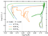 |
Fig. 1. Hertzsprung–Russell (HR) diagram of three selected stellar evolutionary tracks computed with STAREVOL, with different evolutionary paths. The dashed lines show the pre-MS phase |
Stars with 0.75 < MZAMS/M⊙ < 0.85 are massive enough to ignite helium at the RGB tip, undergoing the so-called He-flash. These stars then move to the HB where they undergo stable CHeB. In the fast transition phase, which lasts for ∼1.3 Myr, they may experience several secondary He-flashes (less luminous than the first one) that manifest as loops in the HR diagram. Stars in this mass range retain only tiny envelopes, and they lie on the blue side of the HB during the CHeB. They have higher effective temperatures than more massive stars that retain more massive envelopes (see, e.g., Rood 1973). The mass of the envelope also affects the post-CHeB phase because it is too tiny to allow the shell-burning processes that – in the usual case – force stars to reach the AGB stage. Therefore, these stars with tiny envelopes may completely miss the AGB phase. Moreover, the stellar winds could eject the small envelope during the CHeB phase. Therefore, the star cannot expand and completely avoids the evolution toward the AGB, moving instead to higher luminosities and directly to the planetary nebula phase and WD cooling sequence. This is the evolutionary pattern of AGB-manqué stars
For stars with a higher initial mass that also have higher envelope mass when they reach the RGB tip, the post-CHeB evolution follows the “standard” behavior. During the CHeB, tracks with MZAMS ≥ 0.85 M⊙, have a lower effective temperature, and after this phase, they move to the AGB phase. The advanced AGB phase is characterized by thermal pulses, dredge-up, and strong stellar winds, which determine the duration of this phase. When stellar winds almost totally peel off the envelope, stars move to the planetary nebula phase (sometimes experiencing a last thermal pulse) and finally to the WD cooling sequence
Figure 2 shows all sets of stellar tracks we use in this work to represent stars of the 1P of the four clusters. After the MS, all stars cross the subgiant region and climb the RGB. Subsequently, as described above, stars may follow three different evolutionary paths, depending on the stellar structure at the tip of the RGB. We consider each track complete if the star has an envelope < 0.1 M⊙ during the planetary nebula phase. In this assumption, all our tracks are complete for our purposes (also those with Z = 0.0009 and Y = 0.248415 shown in the top-right panel of Figure 2)
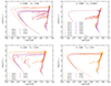 |
Fig. 2. Selected evolutionary tracks of STAREVOL in the HR diagram, representing 1P stars of the four clusters listed in Table 1. Starting from the top-left and going clockwise, tracks are computed with Z = 0.0002, 0.0009, 0.008, and 0.002. Different colors indicate different initial masses. Tracks are shown from their ZAMS to the planetary nebula phase and WD cooling. The little star apex in the label before the masses indicates stars that go to the AGB phase |
The transition masses between the different kinds of evolution and the occurrence of AGB-manqué behavior depend on the initial abundances of helium and metals (as shown in Figures 5 and 6 by Charbonnel & Chantereau 2016). In general, the higher the metal content, the higher the transition mass between stars with the AGB-manqué and AGB evolutionary patterns. On the other hand, for 2P stars, the trend of the transition masses is not linear with the initial helium abundance. For Y < 0.5, the higher the helium, the smaller the transition mass. While, in cases of a very high helium enrichment (i.e., Y > 0.5), the trend can be inverted (see Figure 2 in Chantereau et al. 2016). From the analysis presented in Appendix B, we expect the effect of detailed abundances of elements other than He and which do count in the metal mass fraction Z to be small. We thus expect that the use of 2P abundances derived from the FRMS scenario, as done here or from other scenarios, will not impact the results obtained in this work. For a detailed description of the impact of the helium enrichment on the tracks and the transition masses for different metallicities, we refer the reader to Chantereau et al. (2015) and Charbonnel & Chantereau (2016)
It is worth noticing that the transition masses and the occurrence of the AGB-manqué evolution also depend on the mass-loss in the RGB and HB phases. The mass loss in such phases (particularly on the RGB) is still an open issue and has great uncertainty (e.g., Tailo et al. 2021). Further exploration of the uncertainty related to stellar wind prescriptions is outside the scope of this paper
3. Isochrones
The computation of theoretical isochrones has a long tradition, and several groups have developed their tools to tackle this task (some recent examples are VandenBerg et al. 2014; Georgy et al. 2014; Dotter 2016; Spada et al. 2017; Hidalgo et al. 2018; Nguyen et al. 2022). These tools use smart and efficient methods that exploit the similarities between tracks to obtain accurate isochrones, starting from sets of tracks, which, for obvious reasons, cannot span the space of initial parameters “continuously”. One common key idea adopted in the isochrones building methods is the selection of the so-called equivalent evolutionary points (or “critical points”) along the evolutionary tracks (Simpson et al. 1970; Bertelli et al. 1990, 1994; Girardi et al. 2000; Ekström et al. 2012). An accurate selection of these critical points permits obtaining smooth interpolated tracks and morphologically realistic isochrones without wasting resources in the computation of very big stellar track grids with infinitely small mass steps between each track. Typically, grids of tracks to compute isochrones include a few hundred tracks, not more
It is worth stressing here that a good selection of critical points is not enough to obtain acceptable isochrones. Since stellar tracks with two very close masses may show a very different morphology in the post-RGB phase (as shown in Fig. 1), a specific strategy to treat this aspect accurately must be adopted. Ignoring those transitions in the isochrone building methods will produce wrong isochrones, as the one shown in Fig. 3. In this case, the isochrone in the post-RGB is computed from the interpolations of the two tracks shown without an adapted methodology. This isochrone is a clear example of a “blind” interpolation that produces nonphysical properties, such as a faint (logL < 3) and hot (Teff > 3.8) AGB phase. Because the stars in these phases are bright, their properties impact the integrated colors of a synthetic stellar population. Some of the evolutionary phases affected are short-lived, in which case their impact on average integrated properties is limited, but they nevertheless modify the statistical distributions of colors of equal-age populations of synthetic clusters with finite numbers of stars (a distribution due to the stochastic sampling of the IMF; for examples see Girardi & Bica 1993; Fouesneau & Lançon 2010)
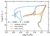 |
Fig. 3. Example of an incorrect isochrone (dashed black line), as obtained when not accounting for the different morphologies of the post-RGB phase of the two tracks used in the interpolation. The isochrone has an age of 14 Gyr. The two tracks used for the interpolation of the post-RGB phases are shown in blue and orange. The initial metallicity is Z = 0.002, and the initial He mass fraction is 0.249. The two tracks shown are reduced tracks obtained following the method described in Section C.1 |
3.1. Isochrone building with SYCLIST
Our building methodology consists of three steps: the creation of reduced stellar track tables, the creation of the “fake” tracks, and the isochrone-building process. All the details are described in Appendix C. In brief, in the first step, we select the equivalent evolutionary points and interpolate between them to create reduced tables. In the second, we create the fake tracks needed to avoid inadequate interpolations between tracks with different post-RGB morphology. These tracks share the evolutionary properties of the two nearest tracks that enclose the transition. For the final step that leads from properly re-sampled tracks to isochrones, we used the SYCLIST code (described in detail in Georgy et al. 2014). Thanks to its flexible design, modifying the equivalent points along tracks and introducing the fake track method did not change the code’s structure. We updated the code to propagate several surface abundances from the STAREVOL stellar tracks to the isochrones, which will be useful for any subsequent computation of detailed synthetic spectra. Our isochrones now include surface abundances of 40 isotopes from 1H to 37Cl, plus all the remaining heavier elements collected in a single variable, “Heavy”. The heavier isotopes (included in the Heavy abundance) could be easily retrieved using the initial element partition adopted since these elements do not evolve in time in our stellar models
3.2. New isochrones
For each set listed in Table 1, we computed new isochrones from 9 Gyr to 14 Gyr, with steps of 0.5 Gyr. Figure 4 shows an example of selected isochrones computed with a fixed initial composition and different ages. The figure shows how, as the age of the isochrones increases, the turn-off becomes fainter and redder, and the star’s position in the HB becomes bluer. The bluer position of the HB at older ages is related to the smaller stellar mass at the RGB tip and the smaller envelope masses that such stars retain in that phase (Bertelli et al. 2008). When the envelope mass is very small, the AGB-manqué evolutionary pattern appears. In this case, stars burn He in a very hot location on the HR diagram and then evolve directly to the planetary nebula, skipping the AGB phase. In Figure 4, all isochrones aged over 13 Gyr show the AGB-manqué behavior (note that these isochrones overlap in the figure because of our isochrone building methodology). While isochrones with ages ≤13 Gyr have a colder HB phase and stars in the AGB phase
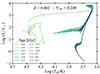 |
Fig. 4. Isochrones with different ages from 8 to 16 Gyr with different colors. The initial abundances are Z = 0.002 and Y = 0.249. Isochrones with 13.5 and 14 Gyr overlap due to our isochrone-building methodology. Therefore, only the one with 13.5 Gyr is visible |
Figure 5 shows selected isochrones with different initial He and two different ages but the same metallicity. Isochrones with different initial He-content run in the HR diagram almost parallel during the MS. As already mentioned, a higher initial He takes to a lower mean opacity and a higher mean molecular weight in the stellar envelope, leading to hotter effective temperatures. Counterintuitively, He-enriched populations are fainter in the MS turn-off because of the shorter MS lifetimes, which indicate a lower mass at the turn-off (Salaris & Cassisi 2005; Bertelli et al. 2008; Chantereau et al. 2015; Cassisi & Salaris 2020). Interestingly, this is also true in the case of very young ages (down to 3 Myr), as shown by Nataf et al. (2020). After the MS, the initial He-content does not affect the morphology of the subgiant branch much. Still, He-enriched populations climb the RGB with higher effective temperatures. The He-content also affects the luminosity tip of the RGB. With an increasing initial He abundance, the brightness of the tip decreases. This is due to the higher central temperatures of the He-enriched models, which take to lower degenerate cores and to a faster rate of growth of the core. Both these effects make the He-flash condition occur with smaller He core masses, hence with lower luminosities (Cassisi & Salaris 2020). After the He-flash, the initial He content affects the isochrones’ morphologies for two reasons. The first is that the He-enriched populations reach the RGB tip with a smaller ratio between the envelope and total mass, mainly due to the smaller MS turn-off masses. The second is that the abundance of He in the stellar envelope during the HB is higher in He-rich stars. They both take the He-enriched populations to have hotter (i.e., bluer) HB than populations with standard He. For the same reasons above, the occurrence of AGB-manqué in a stellar population at a fixed age also depends on the initial He. In Figure 5, isochrones with 9 and 13 Gyr, and with Y < 0.4 have models in the AGB phase, and those with Y = 0.4 have AGB-manqué stars. Finally, models in isochrones with Y = 0.6 just reach the RGB-tip before going to the planetary phase and WD cooling sequence
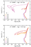 |
Fig. 5. New isochrones computed with ages 9 Gyr and 13 Gyr in the top and bottom panels, respectively. Different colors indicate the different initial He content. All isochrones shown here have Z = 0.0009 |
4. Number ratios
The frequency of AGBs with respect to RGBs and HBs stars is strictly related to multiple populations in GCs (Gratton et al. 2019). Since AGB-manqué stars at certain ages are associated with the He-enriched populations of a cluster (D’Antona et al. 2002; Charbonnel et al. 2013; Chantereau et al. 2016), differences in the initial He enrichment affect the ratios R1 = NAGB/NRGB and R2 = NAGB/NHB (which are proportional to the lifetimes’ ratios of these phases). Our tracks include all the evolution from the ZAMS to the TP-AGB; thus, we can consistently compute and predict values of R1 and R2 for all our isochrones with different ages and initial compositions and compare them with those from the literature obtained from the observed data. The purpose of this comparison is to check the accuracy of our new isochrones, which will be used to compute integrated synthetic spectra in a dedicated work to study distant and not-resolved populations
4.1. Ratios computation
Assuming a certain age, the number of stars, NX, of a population in an evolutionary phase, X, could be computed as follows
 (1)
(1)
where ΔMX is the interval of mass within the selected phase X, Φ(MZAMS) is the initial mass function and MZAMS is the initial stellar mass. By knowing the mass limits of the different phases from our isochrones and assuming a Kroupa initial mass function (Kroupa 2001), we can compute the number ratios R1 and R2 for each isochrone of our sets. We define all the stellar phases in theoretical isochrones by checking the internal properties of the models (i.e., using the same approach described in Sect. C.1). On the other hand, a precise definition of the stellar phases cannot be easily retrieved from observations. In particular, it is difficult to disentangle stars in the RGB and AGB phases, which are often quite overlapped in optical CMDs due to their similar effective temperatures. Therefore, some strategy must be adopted to decouple such stars and break the degeneracy. An interesting methodology has been used by Lagioia et al. (2021), who analyzed photometric data of several GCs from HST. They used far-UV-optical CMDs to break the color degeneracy of RGB and AGB stars, exploiting the property of AGB stars that are significantly brighter than RGB stars in the UV flux. After the selection of the AGB stars, they selected the fainter AGB star in optical CMDs (F814W band) and used that magnitude as a limit for selecting the brighter RGB stars. This methodology ensures a reasonable comparison between stars in the two phases. To compare our theoretical ratios with the empirical ones derived from observational data, we adopt a strategy inspired by Lagioia et al. (2021) to derive stellar numbers of RGB stars. This step is required to compare our R1 number ratios with theirs. Firstly, we selected the luminosity of the early-AGB phase (defined as the onset of the He-shell burning). Then, we used that luminosity as a lower limit to select the mass limit of the most luminous models in the RGB phase. As regards the HB phase, the selected mass limits are the beginning of the CHeB and the beginning of the early-AGB phases. Once the mass limits of each phase are defined, we computed the number ratios R1 and R2 for all the isochrones in our sets. We compute the ratios only for isochrones that populate the AGB, that is, with models that lie in the region of the HR diagram defined by Teff < 3.85 and logL > 3.1, making possible the computation of the ratios. We also associate a statistical Poisson error with the observed ratios when the authors do not provide one. Since the error size depends on the cluster’s number of AGB stars, number ratios of clusters with a few AGBs (such as for Z = 0.0002 and 0.0009 that correspond to NGC 4590 and NGC 6752) have bigger errors. On the modeling side, it is important to say that there are many uncertainties on several physical stellar processes that can change the number counts, such as the mass loss in the RGB and AGB phases, the thermohaline mixing, the semiconvection, stellar rotation, and nuclear rates uncertainties during the CHeB phase. In Appendix B, we show a partial comparison with stellar tracks found in the literature and using the STAREVOL code with different physical assumptions
4.2. Results and comparison with data
The ratios for each initial composition and age are shown in Figure 6 and listed in Table A.1. Our results indicate a general trend for all cases. We find that R1 is proportional to the initial He enrichment, while R2 has an inverse proportionality with the initial He. This is expected since the lifetimes of such phases depend on the initial He and because (dτRGB/dYini)< (dτAGB/dYini)< (dτHB/dYini), where τRGB, τAGB and τHB are the lifetimes of the different phases. An example of the lifetime trends with the initial He is shown by Chantereau et al. (2015) in Figure 3. However, this general trend may change for R1 at older ages (12 − 13 Gyr) due to the AGB lifetimes of the He-enriched populations. In particular, stars close to the AGBm-AGB transition mass (δM < 0.05 M⊙) have shorter AGB lifetimes than stars with a mass well above the transition (δM < 0.05 M⊙)
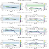 |
Fig. 6. Number ratios versus age, for different initial He content (in different colors). The left column shows R1, while the right column shows R2. Each row indicates the ratios for different initial metallicity (i.e., for different clusters). The dashed horizontal black lines indicate the number ratios for each cluster obtained by Lagioia et al. (2021, L21) from observations. The corresponding 1σ statistical Poisson error is indicated by the blue horizontal area. The dashed blue and red lines indicate R2 results by Constantino et al. (2016), which used data from Piotto et al. (2002, P02) and Sarajedini et al. (2007, S07), respectively. The dashed green line shows values from the collection by Sandquist (2000, S00). The green area in the upper-right panel shows the error associated with the Sandquist (2000) value of the ratio. For clarity purposes, we do not show the statistical errors of all observed values in the other panels, but only those by Lagioia et al. (2021). The other errors have amplitudes similar to those shown here |
We also compare our number ratios with values from the literature obtained from observations. In particular, we compare the R1 ratios with those obtained from observation by Lagioia et al. (2021) because they are retrieved with similar methodologies (as described above). Regarding R2, we compare the ratios with those by Sandquist (2000), Constantino et al. (2016) who computed the ratios from different catalogs (Piotto et al. 2002; Sarajedini et al. 2007), and by Lagioia et al. (2021). The observed values are retrieved by counting all stars in the cluster, thus, without distinguishing between 1P and 2P stars. The comparison is not intended as an attempt to fit the four clusters in detail, but only as a test for our post-RGB tracks and for the new isochrones, which are representative of a simple stellar population (i.e., a coeval population with a certain initial abundance). This check has the aim of verifying whether the current set of evolutionary models, without any fine-tuning, reproduces lifetimes in the various post-RGB phases reasonably well
From the comparison of the number ratios with the observed ones, we find that our R1 and R2 roughly agree within 1σ with observations. There are only two exceptions, one for the R1 ratios computed with Z = 0.008 and the other for the R2 ratios for Z = 0.0002. In the first case, the theoretical ratios are consistently lower than the observed value by 1 or more σ, depending on the initial He. In this case, He-enriched populations seem to reproduce better the observations. In the second case, the R2 values are off the observed value by more than 1σ. However, it is worth noticing that the R2 value presented by Sandquist (2000) for this cluster should be taken with care since the number of AGBs they find is about 5 times higher than those found by other authors (such as Lagioia et al. 2021, who found just 7 AGBs and did not compute the R2 value for this cluster), therefore affecting the ratio value. On the other hand, we find that our R2 ratios also very well agree with other theoretical predictions, which find that R2 should not exceed 0.2 (Cassisi et al. 2014)
Figure 6 also shows the dependence of AGB star occurrences with the initial He enrichment. The maximum age at which AGB stars appear decreases as the initial He increases. However, assuming a different set of input physics for our stellar models may change this threshold age. For instance, including atomic diffusion may change the stars’ lifetimes by up to 10 − 20% (e.g., VandenBerg et al. 2002; Dotter et al. 2017; Borisov et al. 2024). Therefore, the threshold age between the occurrence of AGB-manqué and AGB will change too. This prevents us from using our results to discern the presence of 2P stars in the AGB phase with Yini < 0.3. On the other hand, we can state that in clusters with similar metallicity to those investigated here, the presence of AGB stars at ages above 12 Gyr with Yini ≥ 0.4 is quite unlikely, as already predicted and discussed by several authors (e.g., Charbonnel et al. 2013; Milone et al. 2018; Martins et al. 2021). Finally, Table A.1 lists all the R1 and R2 ratio values and the corresponding errors for each metallicity, age, and initial He enrichment
5. Conclusions
In this paper, we adopted and extended stellar evolution tracks from Charbonnel & Chantereau (2016), Chantereau et al. (2017), and Martins et al. (2021) such as to include lower stellar masses and to fully process late stages of evolution up to the end of the TP-AGB phase. We described the methodology adopted to build morphologically accurate isochrones in the presence of transitions from tracks with a standard evolutionary path through the HB and the AGB, to tracks which lack either the AGB, or both the HB and the AGB. We presented the resulting isochrones for various metallicities, initial He-contents, and ages (spanning from 9 to 14 Gyr). The stellar tracks and the new isochrones are available in the CDS database
For each isochrone, we computed the ratios between the number of AGB stars and the number of RGB stars on one hand and of HB stars on the other. We find a good agreement with observed counts within 1σ for most cases. That means that with the parameters and initial physical processes chosen, our models predict reasonable lifetimes for the different post-RGB evolutionary phases. Varying physical processes, such as overshooting, atomic diffusion, mass loss on the RGB, or rotation, might modify the resulting number ratios, but this should not affect our conclusions on the differential importance of He (as shown in Appendix B)
This work is the first methodological paper of a series that aims to study and characterize remote unresolved stellar populations, which will become more readily available thanks to the James Webb and Euclid space missions. Complete isochrones are the first step for creating integrated synthetic spectra of simulated populations computed with different initial abundances and stellar physical conditions. We have shown that this grid of tracks produces reasonable number ratios of various types of luminous evolved stars, which is a prerequisite for reasonable integrated light fluxes. The set of tracks and the isochrones presented and discussed here will be a reference set to which we will compare results for stellar evolution models with modified assumptions, such as updated initial chemical compositions, modified surface boundary conditions, or the presence of various internal mixing processes
It is worth noting that 1P could be more complex than first thought. In fact, as suggested in the study by Marino et al. (2019), 1P stars in GCs show a potential metallicity spread
Computations start on the Hayashi track at the beginning of the deuterium burning phase on the PMS that we consider as the time zero of the evolution
The not monotonic decrease of X(He) could be due to thermal breath pulses or potential numerical spikes
It is important to use such a small value for ε to avoid incorrect interpolation between the tracks. As explained in Section 3.1, we need to use very tiny dm in the isochrone building to follow the fast evolution after the He-flash, and obtain accurate isochrones
Acknowledgments
The authors acknowledge Christian Boily, Pierre-Alain Duc, Fabrice Martins, Olivier Richard, and Ferreol Soulez for the fruitful discussions that led to the development of the project. This work was supported by the Agence Nationale de la Recherche grant POPSYCLE number ANR-19-CE31-0022. TD is supported by the European Union, ChETEC-INFRA, project no. 101008324. CC thanks the Swiss National Science Foundation (SNF; Project 200021−212160). VB, PC, LM are financed in part by the Coordenação de Aperfeiçoamento de Pessoal de Nível Superior – Brazil (CAPES) – Finance Code 88887.580690/2020-00, the Conselho Nacional de Desenvolvimento Científico e Tecnológico (CNPq) under the grants 200928/2022-8, 310555/2021-3, and 307115/2021-6, and by Fundação de Amparo à Pesquisa do Estado de São Paulo (FAPESP) process numbers 2021/08813-7 and 2022/03703-1. CG has received funding from the European Research Council (ERC) under the European Union’s Horizon 2020 research and innovation programme (grant agreement No 833925, project STAREX)
References
- Amard, L., Palacios, A., Charbonnel, C., et al. 2019, A&A, 631, A77 [NASA ADS] [CrossRef] [EDP Sciences] [Google Scholar]
- Arndt, T. U., Fleischer, A. J., & Sedlmayr, E. 1997, A&A, 327, 614 [NASA ADS] [Google Scholar]
- Bastian, N., & Lardo, C. 2018, ARA&A, 56, 83 [Google Scholar]
- Bastian, N., Cabrera-Ziri, I., & Salaris, M. 2015, MNRAS, 449, 3333 [NASA ADS] [CrossRef] [Google Scholar]
- Bedin, L. R., Piotto, G., Anderson, J., et al. 2004, ApJ, 605, L125 [Google Scholar]
- Bertelli, G., Betto, R., Bressan, A., et al. 1990, A&AS, 85, 845 [NASA ADS] [Google Scholar]
- Bertelli, G., Bressan, A., Chiosi, C., Fagotto, F., & Nasi, E. 1994, A&AS, 106, 275 [NASA ADS] [Google Scholar]
- Bertelli, G., Girardi, L., Marigo, P., & Nasi, E. 2008, A&A, 484, 815 [NASA ADS] [CrossRef] [EDP Sciences] [Google Scholar]
- Böhm-Vitense, E. 1958, Z. Astophys., 46, 108 [Google Scholar]
- Borisov, S., Charbonnel, C., Prantzos, N., Dumont, T., & Palacios, A. 2024, A&A, submitted [arXiv:2403.15534] [Google Scholar]
- Bressan, A., Fagotto, F., Bertelli, G., & Chiosi, C. 1993, A&AS, 100, 647 [NASA ADS] [Google Scholar]
- Cadelano, M., Pallanca, C., Dalessandro, E., et al. 2023, A&A, 679, L13 [NASA ADS] [CrossRef] [EDP Sciences] [Google Scholar]
- Cameron, A. J., Katz, H., Rey, M. P., & Saxena, A. 2023, MNRAS, 523, 3516 [NASA ADS] [CrossRef] [Google Scholar]
- Campbell, S. W., D’Orazi, V., Yong, D., et al. 2013, Nature, 498, 198 [Google Scholar]
- Carretta, E. 2015, ApJ, 810, 148 [Google Scholar]
- Carretta, E., & Bragaglia, A. 2021, A&A, 646, A9 [EDP Sciences] [Google Scholar]
- Carretta, E., Bragaglia, A., Gratton, R. G., et al. 2010, A&A, 516, A55 [NASA ADS] [CrossRef] [EDP Sciences] [Google Scholar]
- Cassisi, S., & Salaris, M. 2020, A&A Rev., 28, 5 [NASA ADS] [CrossRef] [Google Scholar]
- Cassisi, S., Salaris, M., Pietrinferni, A., Vink, J. S., & Monelli, M. 2014, A&A, 571, A81 [NASA ADS] [CrossRef] [EDP Sciences] [Google Scholar]
- Chantereau, W., Charbonnel, C., & Decressin, T. 2015, A&A, 578, A117 [NASA ADS] [CrossRef] [EDP Sciences] [Google Scholar]
- Chantereau, W., Charbonnel, C., & Meynet, G. 2016, A&A, 592, A111 [NASA ADS] [CrossRef] [EDP Sciences] [Google Scholar]
- Chantereau, W., Charbonnel, C., & Meynet, G. 2017, A&A, 602, A13 [Google Scholar]
- Charbonnel, C., & Chantereau, W. 2016, A&A, 586, A21 [NASA ADS] [CrossRef] [EDP Sciences] [Google Scholar]
- Charbonnel, C., Chantereau, W., Decressin, T., Meynet, G., & Schaerer, D. 2013, A&A, 557, L17 [NASA ADS] [CrossRef] [EDP Sciences] [Google Scholar]
- Charbonnel, C., Schaerer, D., Prantzos, N., et al. 2023, A&A, 673, L7 [NASA ADS] [CrossRef] [EDP Sciences] [Google Scholar]
- Choi, J., Dotter, A., Conroy, C., et al. 2016, ApJ, 823, 102 [Google Scholar]
- Coc, A., Uzan, J. P., & Vangioni, E. 2013, arXiv e-prints [arXiv:1307.6955] [Google Scholar]
- Constantino, T., Campbell, S. W., Lattanzio, J. C., & van Duijneveldt, A. 2016, MNRAS, 456, 3866 [Google Scholar]
- D’Antona, F., Caloi, V., Montalbán, J., Ventura, P., & Gratton, R. 2002, A&A, 395, 69 [CrossRef] [EDP Sciences] [Google Scholar]
- D’Antona, F., Bellazzini, M., Caloi, V., et al. 2005, ApJ, 631, 868 [Google Scholar]
- D’Antona, F., Vesperini, E., D’Ercole, A., et al. 2016, MNRAS, 458, 2122 [Google Scholar]
- D’Antona, F., Vesperini, E., Calura, F., et al. 2023, A&A, 680, L19 [NASA ADS] [CrossRef] [EDP Sciences] [Google Scholar]
- Decressin, T., Charbonnel, C., & Meynet, G. 2007a, A&A, 475, 859 [CrossRef] [EDP Sciences] [Google Scholar]
- Decressin, T., Meynet, G., Charbonnel, C., Prantzos, N., & Ekström, S. 2007b, A&A, 464, 1029 [NASA ADS] [CrossRef] [EDP Sciences] [Google Scholar]
- Denissenkov, P. A., & Hartwick, F. D. A. 2014, MNRAS, 437, L21 [Google Scholar]
- D’Ercole, A., D’Antona, F., Carini, R., Vesperini, E., & Ventura, P. 2012, MNRAS, 423, 1521 [Google Scholar]
- de Mink, S. E., Pols, O. R., Langer, N., & Izzard, R. G. 2009, A&A, 507, L1 [NASA ADS] [CrossRef] [EDP Sciences] [Google Scholar]
- Doherty, C. L., Gil-Pons, P., Lau, H. H. B., Lattanzio, J. C., & Siess, L. 2014, MNRAS, 437, 195 [Google Scholar]
- Dorman, B., Rood, R. T., & O’Connell, R. W. 1993, ApJ, 419, 596 [NASA ADS] [CrossRef] [Google Scholar]
- Dotter, A. 2016, ApJS, 222, 8 [Google Scholar]
- Dotter, A., Conroy, C., Cargile, P., & Asplund, M. 2017, ApJ, 840, 99 [Google Scholar]
- Eggleton, P. P., Faulkner, J., & Flannery, B. P. 1973, A&A, 23, 325 [NASA ADS] [Google Scholar]
- Ekström, S., Georgy, C., Eggenberger, P., et al. 2012, A&A, 537, A146 [Google Scholar]
- Ferguson, J. W., Alexander, D. R., Allard, F., et al. 2005, ApJ, 623, 585 [Google Scholar]
- Forestini, M., & Charbonnel, C. 1997, A&AS, 123, 241 [NASA ADS] [CrossRef] [EDP Sciences] [Google Scholar]
- Fouesneau, M., & Lançon, A. 2010, A&A, 521, A22 [NASA ADS] [CrossRef] [EDP Sciences] [Google Scholar]
- Georgy, C., Granada, A., Ekström, S., et al. 2014, A&A, 566, A21 [NASA ADS] [CrossRef] [EDP Sciences] [Google Scholar]
- Gieles, M., Charbonnel, C., Krause, M. G. H., et al. 2018, MNRAS, 478, 2461 [Google Scholar]
- Girardi, L., & Bica, E. 1993, A&A, 274, 279 [NASA ADS] [Google Scholar]
- Girardi, L., Bressan, A., Bertelli, G., & Chiosi, C. 2000, A&AS, 141, 371 [NASA ADS] [CrossRef] [EDP Sciences] [Google Scholar]
- Graboske, H. C., Dewitt, H. E., Grossman, A. S., & Cooper, M. S. 1973, ApJ, 181, 457 [Google Scholar]
- Gratton, R., Bragaglia, A., Carretta, E., et al. 2019, A&A Rev., 27, 8 [NASA ADS] [CrossRef] [Google Scholar]
- Gratton, R. G., D’Orazi, V., Bragaglia, A., Carretta, E., & Lucatello, S. 2010, A&A, 522, A77 [NASA ADS] [CrossRef] [EDP Sciences] [Google Scholar]
- Greggio, L., & Renzini, A. 1990, ApJ, 364, 35 [Google Scholar]
- Grevesse, N., & Noels, A. 1993, in Origin and Evolution of the Elements, eds. N. Prantzos, E. Vangioni-Flam, & M. Casse, 15 [Google Scholar]
- Groenewegen, M. A. T., & de Jong, T. 1993, A&A, 267, 410 [NASA ADS] [Google Scholar]
- Hidalgo, S. L., Pietrinferni, A., Cassisi, S., et al. 2018, ApJ, 856, 125 [Google Scholar]
- Iben, I., & Rood, R. T. 1969, Nature, 223, 933 [NASA ADS] [CrossRef] [Google Scholar]
- Iben, I. Jr., & Faulkner, J. 1968, ApJ, 153, 101 [NASA ADS] [CrossRef] [Google Scholar]
- Iglesias, C. A., & Rogers, F. J. 1996, ApJ, 464, 943 [NASA ADS] [CrossRef] [Google Scholar]
- King, I. R., Bedin, L. R., Cassisi, S., et al. 2012, AJ, 144, 5 [NASA ADS] [CrossRef] [Google Scholar]
- Krause, M., Charbonnel, C., Decressin, T., Meynet, G., & Prantzos, N. 2013, A&A, 552, A121 [NASA ADS] [CrossRef] [EDP Sciences] [Google Scholar]
- Krause, M. G. H., Charbonnel, C., Bastian, N., & Diehl, R. 2016, A&A, 587, A53 [NASA ADS] [CrossRef] [EDP Sciences] [Google Scholar]
- Kroupa, P. 2001, MNRAS, 322, 231 [NASA ADS] [CrossRef] [Google Scholar]
- Lagarde, N., Decressin, T., Charbonnel, C., et al. 2012, A&A, 543, A108 [NASA ADS] [CrossRef] [EDP Sciences] [Google Scholar]
- Lagioia, E. P., Milone, A. P., Marino, A. F., et al. 2021, ApJ, 910, 6 [NASA ADS] [CrossRef] [Google Scholar]
- Lapenna, E., Lardo, C., Mucciarelli, A., et al. 2016, ApJ, 826, L1 [NASA ADS] [CrossRef] [Google Scholar]
- Lind, K., Charbonnel, C., Decressin, T., et al. 2011, A&A, 527, A148 [NASA ADS] [CrossRef] [EDP Sciences] [Google Scholar]
- Marigo, P., Girardi, L., Bressan, A., et al. 2008, A&A, 482, 883 [NASA ADS] [CrossRef] [EDP Sciences] [Google Scholar]
- Marigo, P., Bressan, A., Nanni, A., Girardi, L., & Pumo, M. L. 2013, MNRAS, 434, 488 [Google Scholar]
- Marigo, P., Girardi, L., Bressan, A., et al. 2017, ApJ, 835, 77 [Google Scholar]
- Marino, A. F., Milone, A. P., Yong, D., et al. 2017, ApJ, 843, 66 [NASA ADS] [CrossRef] [Google Scholar]
- Marino, A. F., Milone, A. P., Renzini, A., et al. 2019, MNRAS, 487, 3815 [CrossRef] [Google Scholar]
- Martins, F., Chantereau, W., & Charbonnel, C. 2021, A&A, 650, A162 [NASA ADS] [CrossRef] [EDP Sciences] [Google Scholar]
- McDonald, I., & Zijlstra, A. A. 2015, MNRAS, 448, 502 [Google Scholar]
- Michaud, G., Richer, J., & Richard, O. 2008, ApJ, 675, 1223 [NASA ADS] [CrossRef] [Google Scholar]
- Miglio, A., Brogaard, K., Stello, D., et al. 2012, MNRAS, 419, 2077 [Google Scholar]
- Milone, A. P., & Marino, A. F. 2022, Universe, 8, 359 [NASA ADS] [CrossRef] [Google Scholar]
- Milone, A. P., Marino, A. F., Cassisi, S., et al. 2012, ApJ, 754, L34 [NASA ADS] [CrossRef] [Google Scholar]
- Milone, A. P., Marino, A. F., Bedin, L. R., et al. 2014, MNRAS, 439, 1588 [NASA ADS] [CrossRef] [Google Scholar]
- Milone, A. P., Piotto, G., Renzini, A., et al. 2017, MNRAS, 464, 3636 [Google Scholar]
- Milone, A. P., Marino, A. F., Renzini, A., et al. 2018, MNRAS, 481, 5098 [NASA ADS] [CrossRef] [Google Scholar]
- Milone, A. P., Marino, A. F., Dotter, A., et al. 2023, MNRAS, 522, 2429 [CrossRef] [Google Scholar]
- Mitler, H. E. 1977, ApJ, 212, 513 [NASA ADS] [CrossRef] [Google Scholar]
- Mouhcine, M., & Lançon, A. 2002, A&A, 393, 149 [NASA ADS] [CrossRef] [EDP Sciences] [Google Scholar]
- Nataf, D.~M., Horiuchi, S., Costa, G., et al. 2020, MNRAS, 496, 3222 [NASA ADS] [CrossRef] [Google Scholar]
- Nguyen, C. T., Costa, G., Girardi, L., et al. 2022, A&A, 665, A126 [NASA ADS] [CrossRef] [EDP Sciences] [Google Scholar]
- Palacios, A., Talon, S., Charbonnel, C., & Forestini, M. 2003, A&A, 399, 603 [CrossRef] [EDP Sciences] [Google Scholar]
- Piotto, G., King, I. R., Djorgovski, S. G., et al. 2002, A&A, 391, 945 [NASA ADS] [CrossRef] [EDP Sciences] [Google Scholar]
- Piotto, G., Villanova, S., Bedin, L. R., et al. 2005, ApJ, 621, 777 [Google Scholar]
- Piotto, G., Bedin, L. R., Anderson, J., et al. 2007, ApJ, 661, L53 [NASA ADS] [CrossRef] [Google Scholar]
- Pols, O. R., Tout, C. A., Eggleton, P. P., & Han, Z. 1995, MNRAS, 274, 964 [Google Scholar]
- Prantzos, N., & Charbonnel, C. 2006, A&A, 458, 135 [NASA ADS] [CrossRef] [EDP Sciences] [Google Scholar]
- Prantzos, N., Charbonnel, C., & Iliadis, C. 2017, A&A, 608, A28 [NASA ADS] [CrossRef] [EDP Sciences] [Google Scholar]
- Reimers, D. 1975, Memoires of the Societe Royale des Sciences de Liege, 8, 369 [Google Scholar]
- Renzini, A., Marino, A. F., & Milone, A. P. 2022, MNRAS, 513, 2111 [NASA ADS] [CrossRef] [Google Scholar]
- Rood, R. T. 1973, ApJ, 184, 815 [NASA ADS] [CrossRef] [Google Scholar]
- Salaris, M., & Cassisi, S. 2005, Evolution of Stars and Stellar Populations (Wiley-VCH) [Google Scholar]
- Sandquist, E. L. 2000, MNRAS, 313, 571 [NASA ADS] [CrossRef] [Google Scholar]
- Sarajedini, A., Bedin, L. R., Chaboyer, B., et al. 2007, AJ, 133, 1658 [Google Scholar]
- Schwarzschild, M. 1958, Structure and Evolution of the Stars (Princeton: Princeton University Press) [Google Scholar]
- Siess, L., Dufour, E., & Forestini, M. 2000, A&A, 358, 593 [Google Scholar]
- Simpson, E., Hills, R. E., Hoffman, W., et al. 1970, ApJ, 159, 895 [NASA ADS] [CrossRef] [Google Scholar]
- Spada, F., Demarque, P., Kim, Y. C., Boyajian, T. S., & Brewer, J. M. 2017, ApJ, 838, 161 [NASA ADS] [CrossRef] [Google Scholar]
- Szécsi, D., Mackey, J., & Langer, N. 2018, A&A, 612, A55 [NASA ADS] [CrossRef] [EDP Sciences] [Google Scholar]
- Tailo, M., Milone, A. P., Lagioia, E. P., et al. 2020, MNRAS, 498, 5745 [CrossRef] [Google Scholar]
- Tailo, M., Milone, A. P., Lagioia, E. P., et al. 2021, MNRAS, 503, 694 [NASA ADS] [CrossRef] [Google Scholar]
- Valcin, D., Bernal, J. L., Jimenez, R., Verde, L., & Wandelt, B. D. 2020, J. Comology Astropart. Phys., 2020, 002 [CrossRef] [Google Scholar]
- VandenBerg, D. A., Richard, O., Michaud, G., & Richer, J. 2002, ApJ, 571, 487 [NASA ADS] [CrossRef] [Google Scholar]
- VandenBerg, D. A., Bergbusch, P. A., Ferguson, J. W., & Edvardsson, B. 2014, ApJ, 794, 72 [NASA ADS] [CrossRef] [Google Scholar]
- Vassiliadis, E., & Wood, P. R. 1993, ApJ, 413, 641 [Google Scholar]
- Ventura, P., D’Antona, F., Mazzitelli, I., & Gratton, R. 2001, ApJ, 550, L65 [CrossRef] [Google Scholar]
- Ventura, P., Di Criscienzo, M., Carini, R., & D’Antona, F. 2013, MNRAS, 431, 3642 [Google Scholar]
- Vink, J. S. 2023, A&A, 679, L9 [NASA ADS] [CrossRef] [EDP Sciences] [Google Scholar]
- Wang, Y., Primas, F., Charbonnel, C., et al. 2016, A&A, 592, A66 [NASA ADS] [CrossRef] [EDP Sciences] [Google Scholar]
- Wang, Y., Primas, F., Charbonnel, C., et al. 2017, A&A, 607, A135 [NASA ADS] [CrossRef] [EDP Sciences] [Google Scholar]
- Xu, Y., Goriely, S., Jorissen, A., Chen, G. L., & Arnould, M. 2013a, A&A, 549, A106 [NASA ADS] [CrossRef] [EDP Sciences] [Google Scholar]
- Xu, Y., Takahashi, K., Goriely, S., et al. 2013b, Nucl. Phys., 918, 61 [CrossRef] [Google Scholar]
Appendix A: Additional table
Globular cluster number ratios (R1 and R2) for different ages and initial He enrichment
Appendix B: Grid comparisons
Here, we compare the properties of our tracks with similar grids computed by other authors. This comparison shows the different lifetimes and number ratios between sets of stellar tracks computed with different physical processes and initial chemical abundance
B.1. On the impact of different formation scenarios
Fig. B.1 shows the MS-lifetimes vs. the initial mass (MZAMS), comparing models from different grids with [Fe/H] = −1.5, all representative of the GC NGC 6752 populations. For this comparison, we adopted our model computed with standard Y (labeled FRMS) and with enhanced helium (Y = 0.4, grid FRMS+He). We also adopted new models (SMS) computed in the super-massive stars framework, which will be published in a forthcoming paper. These tracks are computed with standard helium, Y = 0.248, without atomic diffusion and rotation, but with thermohaline mixing on the RGB phase. Stellar tracks are computed from 0.2 to 1 M⊙ and are computed until they reach an age of 15 Gyr. The last grid of models (labeled SMS rot. in the figure) is taken from new models computed in Borisov et al. (2024). These models are also computed in the SMS scenario, with a [Fe/H] = −1.5 and [α/Fe] = +0.3. The tracks include rotation-induced processes, atomic diffusion, penetrative convection, parametric turbulence, and additional viscosity
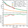 |
Fig. B.1. Top panel: Comparison of the MS lifetimes (τMS) versus the initial mass (MZAMS) for tracks computed with different initial abundances, but the same [Fe/H]. Bottom panel: Relative variation of the MS lifetime with respect to the FRMS scenario (i.e., |
This analysis shows that the effect of detailed abundances of elements that count in the metal mass fraction Z (associated with different self-enrichment scenarios) has a minimal impact with respect to that of He. Specifically, we observe a small relative variation of a few percent when comparing the MS lifetimes of tracks from the FRMS and SMS grids. On the other hand, the variation changes significantly (more than 60%) when comparing them with helium-enriched tracks. From the comparison with the set SMS rot., we find that rotation and atomic diffusion may contribute to variations up to 12% (in this case). Again, helium enrichment has a stronger impact on evolution
B.2. On the differential impact of He on number ratios
We compared the number ratios obtained from our models with those obtained from the grids created by Lagarde et al. (2012) and Choi et al. (2016) to understand how different processes impact them. We chose these two grids because they are similar to our sets of tracks, as they compute the full evolution from the ZAMS to the TP-AGB phases. In this analysis, we focused on comparing the impact of rotation with that of helium
Fig. B.2 shows the comparison between the number ratios R1 and R2 with respect to the initial mass of stars. The number ratios are derived from the evolutionary lifetimes of each track using the same critical points selection method, described in Sec. C.1. The comparison reveals that the impact of stellar rotation on number ratios is relatively small. In fact, by analyzing the largest variations for the same initial mass, it was found that nonrotating and rotating tracks differ by less than 0.1 and 0.04 for R1 and R2, respectively, for the Lagarde et al. (2012) grids. Similarly, for the Choi et al. (2016) tracks, the difference is less than 0.04 and 0.02 for R1 and R2, respectively. On the other hand, a He enrichment of 0.15 in the initial composition (FRMS models) leads to variations greater than 0.2 and about 0.06 in the R1 and R2 values, respectively. It is worth noticing that the largest rotation-related variation for the MIST and Lagarde grids is seen for models with MZAMS > 1.4 M⊙. These models reach the AGB phase at around 2 Gyr, which is much younger than the age of GCs. Finally, according to the models presented in Lagarde et al. (2012), the difference between nonrotating and rotating tracks is negligible for stars with a mass of 0.85 solar masses. Unfortunately, Lagarde et al. (2012) stellar track database4 does not provide models with masses below 0.85 M⊙, focusing instead on the intermediate-mass range. On the other hand, the MIST5 database does not contain rotation models for stars with masses below 1.3 solar masses (Choi et al. 2016)
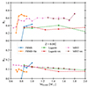 |
Fig. B.2. Comparison of the R1 and R2 ratios for different grids of tracks in the top and bottom panels, respectively. All the values are computed from tracks with Z = 0.002. Continuous lines indicate tracks presented in this work. The FMRS tracks have a standard He (Y = 0.249) and [α/Fe] = +0.3. Tracks FMRS+He are computed with Y = 0.4. Dashed lines show models from Lagarde et al. (2012) with (Lagarde rot.) and without rotation (Lagarde). All these tracks have Y = 0.25 and [α/Fe] = 0. Dotted lines show the MIST models from Choi et al. (2016), with (MIST rot.) and without rotation (MIST). The models are computed with Y = 0.252 and [α/Fe] = 0 |
Appendix C: Isochrone building methods
The method we adopted to build our new isochrones consists of three steps. The first is the selection of critical points and the construction of reduced stellar track tables. The second consists of the creation of the fake track when needed. The last one regards the isochrone building performed with SYCLIST. We present all the important details in the following sections
C.1. First-step – New critical points selection
From each evolutionary track, we create reduced tables containing 500 points selected to describe the whole evolution from the ZAMS to the luminosity tip of the RGB or AGB phases. Firstly, we determine the critical points (cp) that split the different evolutionary phases (see also Ekström et al. 2012; Chantereau et al. 2015). Our selection of the critical points is optimized to sample all the characteristic morphological features of low-mass star tracks in the HR diagram, and represent an updated version of that presented by Chantereau et al. (2015). For stellar tracks that end their evolution after the RGB tip, we select five cps, while for those that ignite helium and evolve in the HB, we select ten cps. The critical points are selected as follows:
-
1.
beginning of the main-sequence (i.e., ZAMS), selected when in the star’s center X(Hini)−X(H)< 0.003, where X(Hini) is the initial hydrogen abundance in mass fraction;
-
2.
MS turn-off point, when central X(H)=0.05;
-
3.
MS-end, when central X(H)< 10−3;
-
4.
bottom of the RGB phase, which is defined as the moment when the mass of the convective envelope is more than 25% of the star’s total mass;
-
5.
tip of the RGB, that is the most luminous point of the RGB phase;
-
6.
first helium luminosity peak after He-flash;
-
7.
beginning of the CHeB phase, when central X(He)< 0.98;
-
8.
end of the CHeB phase, when central X(He)< 0.05;
-
9.
bottom (beginning) of the early-AGB phase, when two burning shells coexist
-
10.
Maximum luminosity (tip) of the TP-AGB phase
Figure C.1 shows the critical points selected for three tracks with different evolutionary paths, as discussed in Section 2.3. The selection of the critical points ensures that the secondary points (selected as described below) are evolutionary equivalent between all tracks
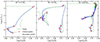 |
Fig. C.1. HR diagram of selected tracks with 0.75, 0.8, and 0.85 M⊙ in the left-hand, middle, and right-hand panels, respectively. The tracks are computed with Z = 0.002 and Y = 0.249. The continuous lines show the evolutionary phases we include in the isochrones computation, while dashed lines indicate the pre-MS and the planetary nebula phases (excluded from the computations). Red diamonds and blue circles show the critical points (marked by a number) and the secondary interpolated points, respectively |
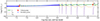 |
Fig. C.2. Evolution of the luminosity vs. time during the AGB phase of a MZAMS = 0.85 M⊙ track with Z = 0.002 and Y = 0.249. Red and blue points indicate the critical and secondary points, respectively. The thin purple and orange lines show the evolution of the luminosity provided by H- and He-burning, respectively |
To determine the secondary equivalent points, we interpolate all intervals between two critical points as follows:
-
We use 25 points to sample both [cp1-cp2] and [cp2-cp3] intervals, with linear steps in central X(H) abundance
-
40 points to interpolate the interval [cp3-cp4], with linear steps in time
-
40 points to interpolate between [cp4-cp5], in equal steps of log L
-
We select 80 and 65 points in the intervals [cp5-cp6] and [cp6-cp7], respectively. We use equal steps in time to perform the interpolation
-
For the interval [cp7-cp8] (i.e., CHeB phase), we use 50 points with equal steps in the cumulative sum of the central He abundance, X(He). This assures a monotonic trend of the interpolating variable6
-
From the end of the CHeB to the beginning of the AGB phase (i.e., interval [cp8-cp9]), we select 75 points with linear steps in time
-
Finally, for the interval [cp9-cp10] that corresponds to the AGB phase, we use 100 points with equal steps of the cumulative sum of log L. To simplify the difficult interpolation of the TP-AGB phase, we pick only the most luminous points of each inter-pulse quiescent phase in our collection of secondary points, as shown in Figure C.2. Such a simplified approach has been used by other authors in the literature (such as Bertelli et al. 1990; Mouhcine & Lançon 2002; Marigo et al. 2008), and is opposed to other approaches which instead add the thermal pulses in isochrones a posteriori (Marigo et al. 2017)
For the stars that do not go through the He-burning phase, the last line of their evolution, corresponding to the fifth cp (i.e., RGB-tip), is repeated up to line 500, so we keep the same size for all the reduced tables
C.2. Second-step – fake star creation process
The second step for computing smooth isochrones consists of the creation of fake stellar evolution tracks. These tracks are created to cure the quick change of behavior between tracks that go to the planetary nebula phase just after the RGB tip and those that experience the He-flash (we refer to this transition as RGBT-HB), and the transition between tracks that evolve as AGB-manqué and those that go to the standard AGB phase (transition name AGBm-AGB). In both cases, the mass interval in which the change of behavior happens is ΔM < 0.05 M⊙. An example is shown in Figure C.1
The main idea behind the fake track method is to replace the real transition (which could be known only by computing a denser grid of tracks) with an abrupt transition that occurs at an initial mass almost equal to the initial mass of one of the available tracks. The fake track shares the evolutionary properties with each of the two nearest tracks, which enclose the transition. For the sake of simplicity, we use A to refer to the track with the mass above the transition and B to refer to the track with the mass below. For the stellar properties, we use the subscript to indicate which track we refer to (e.g., MA is the initial mass of the track above). For both transitions, we assume that the fake track has a mass Mfake = MA − ε, where ε = 10−11 M⊙ 7
For the first transition (i.e., RGBT-HB), we assume that the fake star follows the evolution of the track A until the RGB tip. Then, we cut all the evolution after the tip, thus assuming that the fake star has the same post-RGB tip evolution as the track B. All the evolutionary properties (also time) of the fake track are exactly the same as the track A, except for the initial mass that is smaller by ε. Things are a bit more complex for the second transition, AGBm-AGB. As before, the fake track follows the evolution of the track A until the RGB tip. After the tip, we assume that the fake star follows the evolution of the track B. The time is the only fake star property that remains the same as that of track A for the whole evolution. An example of fake track reconstruction for the two transitions (RGBT-HB and AGBm-AGB) is shown in Figure C.3. The Figure also shows the two tracks closer to the transition
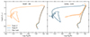 |
Fig. C.3. Two examples of fake tracks (dashed black lines) created to avoid the interpolation between tracks with different evolutionary paths. The orange line shows the track with the mass above the transition (track A), and the blue line indicates the track with the mass below the transition (track B). The left-hand panel shows the fake track created for the transition RGBT-HB (enclosed by tracks with 0.75 and 0.8 M⊙), while the right-hand panel shows the fake track for the AGBm-AGB transition (enclosed by tracks with 0.8 and 0.85 M⊙). All the tracks are computed with Z = 0.002 and Y = 0.249. See details on the fake track creations in the text |
This approach implies that we are assuming that all the tracks between MB and MA evolve in the same way as track B, and the transition between the two evolutionary paths happens in a dm = ε M⊙. Creating and adding the fake track to the collection of tracks adopted to build isochrones assures that we do not interpolate between tracks with different paths and, therefore, permits the computation of isochrones with more reliable morphologies, which do not show strange artifacts, like those shown in Figure 3
Criterion of AGB selection. The criterion chosen in order to detect the occurrence of AGB-manqué evolution is fundamental to properly applying the fake track methodology. We adopted the following check to detect the AGBm behavior: 1- Check the occurrence of at least two thermal pulses. If they are present, proceed to step 2; otherwise, AGBm is detected. 2- Check if the pulse positions in the HR diagram satisfy the following Teff < 3.85 and logL > 3.1. If yes, standard AGB stars are detected; otherwise, AGBm is detected. Other criteria based on other stellar properties, such as the envelope mass vs total mass ratio (Charbonnel et al. 2013), or the central degeneracy at the RGB tip (Cassisi et al. 2014), may help. Still, they do vary with the initial composition and mass. Therefore, it is difficult to establish a general criterion
C.3. Third-step – Isochrone building
SYCLIST uses an adaptive mass step (dm) for the isochrone building process. The mass step is iteratively reduced when the difference between two sequential points of the isochrone satisfies one of the following conditions: δlogTeff > 0.02 or δlogL > 0.02. When the condition is hit, the code recomputes the new mass point with a reduced dm. A minimum mass step (dmmin) is imposed to prevent the code from diverging to infinitesimal dm, avoiding never-ending computations. In fast evolutionary phases, such as after the He-flash, a very small mass step is required to follow that phase properly. We found that dmmin = 10−10 is good enough to interpolate the fast phases and to build good isochrones. We stress here that the choice of an ε < dmmin is critical to minimize the chances of interpolation between a track above the transition and the fake one, as described in Section C.2
Isochrones near the transition masses. The fake tracks should be used carefully to avoid wrong interpolation in the isochrone building process. To properly use fake tracks, it is important to check the age at the tip of the RGB. The fake track should be included in the collection of tracks used to compute isochrones only if the isochrone age is enclosed by the ages at the RGB tip of the two tracks with different behaviors. Figure C.4 shows a result of the blind usage of fake tracks. In this case, the isochrone in the post-RGB part should be interpolated between the two tracks with 0.90 and 0.95 M⊙. Including the fake track, mixed up the interpolation algorithm, and create the wrong interpolation. Therefore, to obtain accurate isochrones, it is important to use fake tracks only when needed
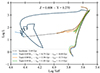 |
Fig. C.4. Example of the wrong use of the fake track in the interpolation to build an isochrone of 13.5 Gyr (indicated by the dashed black line). The two interpolated tracks are shown in blue and orange, while the correct interpolation should be done between the orange and green tracks. The metallicity is 0.008, and the He content is 0.27 |
All Tables
Initial chemical composition and α enhancement of our stellar tracks for each cluster
Globular cluster number ratios (R1 and R2) for different ages and initial He enrichment
All Figures
|
Fig. 1. Hertzsprung–Russell (HR) diagram of three selected stellar evolutionary tracks computed with STAREVOL, with different evolutionary paths. The dashed lines show the pre-MS phase |
| In the text | |
|
Fig. 2. Selected evolutionary tracks of STAREVOL in the HR diagram, representing 1P stars of the four clusters listed in Table 1. Starting from the top-left and going clockwise, tracks are computed with Z = 0.0002, 0.0009, 0.008, and 0.002. Different colors indicate different initial masses. Tracks are shown from their ZAMS to the planetary nebula phase and WD cooling. The little star apex in the label before the masses indicates stars that go to the AGB phase |
| In the text | |
|
Fig. 3. Example of an incorrect isochrone (dashed black line), as obtained when not accounting for the different morphologies of the post-RGB phase of the two tracks used in the interpolation. The isochrone has an age of 14 Gyr. The two tracks used for the interpolation of the post-RGB phases are shown in blue and orange. The initial metallicity is Z = 0.002, and the initial He mass fraction is 0.249. The two tracks shown are reduced tracks obtained following the method described in Section C.1 |
| In the text | |
|
Fig. 4. Isochrones with different ages from 8 to 16 Gyr with different colors. The initial abundances are Z = 0.002 and Y = 0.249. Isochrones with 13.5 and 14 Gyr overlap due to our isochrone-building methodology. Therefore, only the one with 13.5 Gyr is visible |
| In the text | |
|
Fig. 5. New isochrones computed with ages 9 Gyr and 13 Gyr in the top and bottom panels, respectively. Different colors indicate the different initial He content. All isochrones shown here have Z = 0.0009 |
| In the text | |
|
Fig. 6. Number ratios versus age, for different initial He content (in different colors). The left column shows R1, while the right column shows R2. Each row indicates the ratios for different initial metallicity (i.e., for different clusters). The dashed horizontal black lines indicate the number ratios for each cluster obtained by Lagioia et al. (2021, L21) from observations. The corresponding 1σ statistical Poisson error is indicated by the blue horizontal area. The dashed blue and red lines indicate R2 results by Constantino et al. (2016), which used data from Piotto et al. (2002, P02) and Sarajedini et al. (2007, S07), respectively. The dashed green line shows values from the collection by Sandquist (2000, S00). The green area in the upper-right panel shows the error associated with the Sandquist (2000) value of the ratio. For clarity purposes, we do not show the statistical errors of all observed values in the other panels, but only those by Lagioia et al. (2021). The other errors have amplitudes similar to those shown here |
| In the text | |
|
Fig. B.1. Top panel: Comparison of the MS lifetimes (τMS) versus the initial mass (MZAMS) for tracks computed with different initial abundances, but the same [Fe/H]. Bottom panel: Relative variation of the MS lifetime with respect to the FRMS scenario (i.e., |
| In the text | |
|
Fig. B.2. Comparison of the R1 and R2 ratios for different grids of tracks in the top and bottom panels, respectively. All the values are computed from tracks with Z = 0.002. Continuous lines indicate tracks presented in this work. The FMRS tracks have a standard He (Y = 0.249) and [α/Fe] = +0.3. Tracks FMRS+He are computed with Y = 0.4. Dashed lines show models from Lagarde et al. (2012) with (Lagarde rot.) and without rotation (Lagarde). All these tracks have Y = 0.25 and [α/Fe] = 0. Dotted lines show the MIST models from Choi et al. (2016), with (MIST rot.) and without rotation (MIST). The models are computed with Y = 0.252 and [α/Fe] = 0 |
| In the text | |
|
Fig. C.1. HR diagram of selected tracks with 0.75, 0.8, and 0.85 M⊙ in the left-hand, middle, and right-hand panels, respectively. The tracks are computed with Z = 0.002 and Y = 0.249. The continuous lines show the evolutionary phases we include in the isochrones computation, while dashed lines indicate the pre-MS and the planetary nebula phases (excluded from the computations). Red diamonds and blue circles show the critical points (marked by a number) and the secondary interpolated points, respectively |
| In the text | |
|
Fig. C.2. Evolution of the luminosity vs. time during the AGB phase of a MZAMS = 0.85 M⊙ track with Z = 0.002 and Y = 0.249. Red and blue points indicate the critical and secondary points, respectively. The thin purple and orange lines show the evolution of the luminosity provided by H- and He-burning, respectively |
| In the text | |
|
Fig. C.3. Two examples of fake tracks (dashed black lines) created to avoid the interpolation between tracks with different evolutionary paths. The orange line shows the track with the mass above the transition (track A), and the blue line indicates the track with the mass below the transition (track B). The left-hand panel shows the fake track created for the transition RGBT-HB (enclosed by tracks with 0.75 and 0.8 M⊙), while the right-hand panel shows the fake track for the AGBm-AGB transition (enclosed by tracks with 0.8 and 0.85 M⊙). All the tracks are computed with Z = 0.002 and Y = 0.249. See details on the fake track creations in the text |
| In the text | |
|
Fig. C.4. Example of the wrong use of the fake track in the interpolation to build an isochrone of 13.5 Gyr (indicated by the dashed black line). The two interpolated tracks are shown in blue and orange, while the correct interpolation should be done between the orange and green tracks. The metallicity is 0.008, and the He content is 0.27 |
| In the text | |
Current usage metrics show cumulative count of Article Views (full-text article views including HTML views, PDF and ePub downloads, according to the available data) and Abstracts Views on Vision4Press platform.
Data correspond to usage on the plateform after 2015. The current usage metrics is available 48-96 hours after online publication and is updated daily on week days.
Initial download of the metrics may take a while.