| Issue |
A&A
Volume 689, September 2024
|
|
|---|---|---|
| Article Number | A180 | |
| Number of page(s) | 9 | |
| Section | Numerical methods and codes | |
| DOI | https://doi.org/10.1051/0004-6361/202451423 | |
| Published online | 12 September 2024 | |
DIES: Parallel dust radiative transfer program with the immediate re-emission method
Department of Physics,
PO Box 64, University of Helsinki,
00014
Helsinki,
Finland
Received:
8
July
2024
Accepted:
10
August
2024
Abstract
Context. Radiative transfer (RT) modelling is a necessary tool in the interpretation of observations of the thermal emission of interstellar dust. It is also often part of multi-physics modelling. In this context, the efficiency of radiative transfer calculations is important, even for one-dimensional models.
Aims. We investigate the use of the so-called immediate re-emission (IRE) method for fast calculation of one-dimensional spherical cloud models. We wish to determine whether weighting methods similar to those used in traditional Monte Carlo simulations can speed up the estimation of dust temperature.
Methods. We present the program DIES, a parallel implementation of the IRE method, which makes it possible to do the calculations also on graphics processing units (GPUs). We tested the program with externally and internally heated cloud models, and examined the potential improvements from the use of different weighted sampling schemes.
Results. The execution times of the program compare favourably with previous programs, especially when run on GPUs. On the other hand, weighting schemes produce only limited improvements. In the case of an internal radiation source, the basic IRE method samples the re-emission well, while traditional Monte Carlo requires the use of spatial importance sampling. Some noise reduction could be achieved for externally heated models by weighting the initial photon directions. Only in optically very thin models does weighting – such as the proposed method of forced first interaction – result in noise reduction by a factor of several.
Conclusions. The IRE method performs well for both internally and externally heated models, typically without the need for any additional weighting schemes. With run times of the order of one second for our test models, the DIES program is suitable even for larger parameter studies.
Key words: radiative transfer / methods: numerical / ISM: clouds / dust, extinction
Corresponding author; This email address is being protected from spambots. You need JavaScript enabled to view it.
© The Authors 2024
 Open Access article, published by EDP Sciences, under the terms of the Creative Commons Attribution License (https://creativecommons.org/licenses/by/4.0), which permits unrestricted use, distribution, and reproduction in any medium, provided the original work is properly cited.
This article is published in open access under the Subscribe to Open model. This email address is being protected from spambots. You need JavaScript enabled to view it. to support open access publication.
1 Introduction
The first goal of dust radiative transfer (RT) modelling is to determine the temperatures of the dust grains. RT calculations provide information about the radiation field intensity at each position or cell, which corresponds to the spatial discretisation of the model. If dust grains are sufficiently large (have sufficient heat capacity), they can be described using an equilibrium temperature, which results from the balance of absorbed and emitted energies and depends on the assumed optical properties of the grains (Li & Draine 2001; Draine 2003). In the conditions of interstellar clouds, the energy is absorbed mainly at wavelengths from ultraviolet (UV) to near-infrared (NIR) or even mid-infrared (MIR), where the optical depths can be high and scattering is important for the transfer of energy. In contrast, dust re-emits the energy at far-infrared (FIR) wavelengths where the objects are often optically thin. Thus, the calculations need to consider a wide range of wavelengths.
The dust RT problem is typically solved with the Monte Carlo method, by simulating the emission of photons and by following their travel until they are absorbed or leave the model volume (Gordon et al. 2017; Steinacker et al. 2013). For practical reasons, the large number of real photons is divided into a smaller number of photon packages that can be simulated in a computer. The calculations can be divided into iterations, where the radiation field is estimated using up-to-date information on the radiation sources, including the emission from the dust with its current estimated temperatures. When the simulation step has been finished, the knowledge of the radiation field is used to update the dust temperatures in every cell. If the dust re-emission is a significant component of the radiation field, the process needs to be repeated until the temperatures converge (Juvela 2005). In the following, we refer to this approach as the traditional Monte Carlo (TMC) method.
The run times are affected especially by the high optical depths at short wavelengths. Frequent scatterings and the potentially very short free paths mean that the information of the radiation field propagates only slowly through the medium. The time needed to follow a single photon package is a steep function of the optical depth. Furthermore, if hot dust (with significant re-emission) fills a small part of the volume, the simulation of re-emission can become very inefficient. If photon packages are generated at random locations, few of those will correspond to any significant emission. This can happen even in spherically symmetric models, when a central radiation source is surrounded by optically thick but geometrically thin layers of hot dust (Juvela 2005). The sampling of the radiation field can also become poor in the innermost cells in externally heated models, because few of the photon packages initiated at the cloud surface are likely to hit the smallest cells in the centre.
Some of the problems listed above can be alleviated by weighted sampling, where we adjust some of the probability distributions in the Monte Carlo simulation and correspondingly adjust the weight of the photon packages (i.e. the number of real photons they contain). For example, external radiation could be simulated using photon packages that are directed preferentially towards the model centre. This improves the accuracy of the radiation field estimates in the small inner cells. Juvela (2005) examined such weighting schemes in the context of TMC and one-dimensional models. Weighting was applied to the initial positions and directions of the photon packages, as well as the directions of scattered photons. As a special case, it was demonstrated that weighting can also be used to overcome the poor propagation of individual photon packages, up to arbitrarily high optical depths (effectively recovering the diffusion approximation).
One attribute of Monte Carlo simulations that has been examined by several papers is the free path, the distance that a photon package travels before interacting with the medium. In a Monte Carlo program, the random free paths can be calculated based on the optical depth for absorption or optical depth for scattering. Krieger & Wolf (2023) argued in favour of the latter approach when attempting to improve the estimates for the flux that penetrates through high optical depths. The free path is just another probability distribution and can be modified in even more complex ways (Baes et al. 2016; Camps & Baes 2018). However, when sampling is improved in one part of the model, it usually deteriorates in other parts. Thus, the goal of weighted sampling could be either to minimise the maximum errors globally or to minimise the errors for a specific purpose, such as to better estimate the scattered light from a specific model region (Baes et al. 2016; Krieger & Wolf 2024). In many TMC programs, the energy absorption is calculated continuously, with updates made to every cell along the photon path between discrete scattering events (Lucy 1999; Juvela 2005). This ensures lower noise for the temperature estimates, especially in regions of low optical depth.
Bjorkman & Wood (2001) presented a different version of the Monte Carlo scheme, where absorptions are treated as discrete events. After each interaction, the temperature of the absorbing cell is updated and the absorbed energy is immediately reradiated. The new photon package retains the same energy but is given a new random frequency that reflects the probability distributions associated with the temperature change. Because of the discrete locations of the absorption events, the method may suffer from poorer sampling of regions of low optical depth. On the other hand, as the simulation follows the actual flow of energy, the dust emission is automatically better sampled in regions where most of the re-emission takes place (i.e. where dust is hot). In the following, we refer to the Bjorkman & Wood (2001) immediate re-emission method as the IRE method. Juvela (2005) made some comparisons between the TMC and IRE calculations in the case of spherically symmetric and mostly optically thick models. The methods were found to exhibit a comparable performance, although TMC included some non-standard improvements. These included the use of weighted sampling and the so-called reference field method (to decrease noise) and accelerated Monte Carlo (to speed up temperature convergence over iterations). This suggests that the IRE method can be a good way to estimate dust temperatures, at least if stochastic heating can be ignored. Since the method involves a temperature update after each absorption event, it is not clear whether or how IRE could be implemented efficiently in the case of stochastic heating, where the temperature updates are inherently much more expensive (Desert et al. 1986; Draine & Li 2001; Camps et al. 2015). IRE could nevertheless be a good option to be combined for example with the modelling of chemical cloud evolution, where fast RT is needed and knowledge of equilibrium dust temperatures may be sufficient (Sipilä et al. 2020; Chen et al. 2022).
In this paper, we present a new RT program, ‘dust interactions of emission and scattering’ (DIES), which implements the IRE algorithm for parallel computations on both multi-core central processing units (CPUs) and graphics processing units (GPUs)1. We use a series of test problems to investigate the performance of the IRE method and to study whether or not IRE can be enhanced with the use of weighted sampling, as in the case of the TMC methods.
The paper is organised as follows. The IRE method and the weighting schemes are described in Sect. 2. A series of test cloud models are presented and potential improvements from weighted sampling are quantified in Sect. 3. The results are discussed in Sect. 4 before listing the main conclusions in Sect. 5.
2 Methods
2.1 Basic IRE method
The implementation of the IRE method in DIES follows the description in Bjorkman & Wood (2001), in the context of models discretised into spherical cells or shells. There are two potential sources of radiation, an external isotropic radiation field and a point source at the centre of the model.
In the basic version, the total emission per unit time from each of these sources is divided between N photon packages of equal energy. We keep track of the free paths for scattering and for absorptions separately. Both are initialised with random values of optical depth,
 (1)
(1)
where u1 and u2 are independent uniform random numbers, 0 ≤ u ≤ 1. The initial frequency of a photon package is generated from the probability distribution dictated by the source spectrum. We use precalculated lookup tables so that a uniform random number can be quickly mapped to a random frequency within the source spectrum.
Thanks to the model symmetry, the photon package entering from the background can be always initialised at the position (x, y, z) = (0, 0, −R0), where R0 is the outer radius of the model cloud. The angle θ with respect to the normal of the surface (the normal vector pointing inwards) is generated as
 (2)
(2)
with another uniform random number u3. The resulting initial direction is
 (3)
(3)
The rotation angle ϕ is in principle uniformly distributed over 0 ≤ ϕ < 2π, but the value is irrelevant given the model symmetry. For photons emitted by the central source, the procedure is the same, except that µ = cos θ now has a uniform distribution in the range −1 ≤ cos θ ≤ 1.
A photon package is followed in its original direction one cell at a time, and the remaining free paths are correspondingly updated:
 (4)
(4)
where l is the step length, κA,ν and κA,ν are the dust absorption and scattering coefficients (per mass for the current frequency), and p is the density of the cell.
If τS becomes negative before the end of the step (and before τA becomes zero), the step is truncated to the position where τS reaches zero. The photon package is scattered in a new direction according to the dust scattering function ϕv, and both τA and τS are assigned new random values from Eq. (1).
If τA becomes negative before the end of the step (and before τS becomes zero), the step is truncated to the position where τA reached zero. The energy of the photon package is absorbed into the current cell, and the temperature of the cell is updated. The same amount of energy is then re-emitted by creating a new photon package in the same position with a random direction (uniform probability over the full solid angle). The frequency for the photon package is generated from the probability distribution that corresponds to the difference between the emission spectra at the new and old temperatures. Both the new dust temperature and the resulting new frequency are obtained using precalculated lookup tables. Finally, both τA and τS are again given new values according to Eq. (1). The calculation ends when all photon packages from the background and from the point source have been followed until they exit the model volume.
Weighted probability distributions and their parameters.
2.2 Weighted sampling
We tested weighted sampling for five probability distributions that appear in the Monte Carlo simulation. These can be divided to the weighting of directional and distance probability distributions. The options (cf. Table 1) are described below.
The weighting means that the original probability distribution is replaced with a new distribution from which the direction or distance is generated. This change is compensated by adjusting the relative weight of the photon package (i.e. changing the number of true photons that it contains). The weighting factor is the ratio between the original and the modified probabilities that are estimated using the generated value of the variable (i.e. a specific direction or value of a free path). Therefore, alternative distribution must be positive for all valid variable values, and the probability ratio should have only a moderate range of values below and above one in order to avoid noise spikes caused by occasionally very large weight factors. The goal of the weighting is to increase the sampling (decrease the noise) in some parts of the parameter space, especially those where the noise would otherwise be the largest.
2.2.1 Directional weighting
The probability distributions for the direction of photon packages appear in the initialisation of background radiation, the direction of re-emitted photons, and the direction of scattered photons. Because of the spherical symmetry, weighting is not applied to the photon packages from the central source, where the distribution is always isotropic.
When a spherical model is illuminated by external radiation, the smaller projected size of the innermost cells results in higher temperature errors there. The problem may be alleviated by directing the photon packages preferentially towards the model centre. We implemented this by replacing the default direction distribution  with
with  . Each photon package is correspondingly weighted by a factor
 (5)
(5)
using here the current realisation of the µ value. Thus, the value kbg = 0.5 corresponds to the original, unweighted case, and values kbg < 0.5 result in more photon packages being directed towards the central regions of the model.
We can similarly modify the direction of the photon packages after each interaction with the medium. In the case of re-emission, we replace the original isotropic distribution of directions with a Henyey–Greenstein function (Henyey & Greenstein 1941),
 (6)
(6)
In the case of external heating, the direction µ = cos θ is measured with respect to the direction towards the model centre, and in the case of a central point source with respect to the opposite direction. Thus, with positive values of the asymmetry parameter 𝑔A = 〈cos θ〉, photon packages are sent preferentially in the direction away from the original source. In particular, in this way, photon packages from the external radiation field should have a greater chance of reaching the model centre.
The procedure is similar for scattered photons, except that the original distribution of directions is not isotropic but depends on the direction of the photon package before the scattering event and the dust scattering function. We use Henyey–Greenstein functions for both of these. If the scattering angle is µ = cos θ relative to the original direction of propagation and µ′ = cos θ′ is relative to the radial reference direction, the weight is now the ratio of the two Henyey–Greenstein probabilities,
 (7)
(7)
Here 𝑔 is the asymmetry parameter of the dust scattering function and ??S is the parameter chosen for the weighted sampling.
If both the remission and scattering directions are weighted strongly towards the model centre (and the free paths are short), it is possible for a photon package to remain trapped within that region. As a safeguard, DIES will terminate a photon package if its weight has decreased by ten orders of magnitude. If the trapping is caused by the weighting, the limit will be reached after some tens of scattering or re-emission events. However, such strong weighting will also almost certainly result in higher noise in the temperature estimates.
2.2.2 Weighting of free paths
The remaining weighting options concern the free paths, where the goals depend on the model optical depths. When optical depths are high, one could penetrate layers of high optical depth more efficiently by biasing the distribution to contain a greater number of long free paths. Conversely, if the medium is optically thin, shorter free paths could mean more frequent absorption events (for photon packages of smaller weight) and thus lower noise.
The original probability distribution of the free path is p(τ) = e−τ, when expressed in units of the optical depth. We implemented the weighting separately for absorption and scattering events. We use a simple scaling with a constant k (kA for absorption and kS for scattering). The modified probability distribution is p′(τ) = e−kτ, meaning that values k > 1 lead to shorter average free path, and the relative weight of a photon package is
 (8)
(8)
Some tests were made with density-dependent factors, where k is a linear function of log n, based on the local density n. The lowest densities corresponded to the largest values of k (preferring short free paths), and thus induce more absorption events in low-density regions.
The final option concerning free paths could be called forced first interaction (FFI), in analogy to the method of forced first scattering that is often used in calculations of scattered light (Mattila 1970; Witt 1977). This could be useful for models of low optical depth, where a large fraction of the photon packages would not otherwise interact with the medium at all. The method requires additional work to first calculate the total optical depth τ0 along the original photon direction. The normal cumulative probability distribution of free paths, P(τ) = 1 − e−τ , is replaced with the conditional version
 (9)
(9)
and the original formula of free paths is replaced with
![Mathematical equation: $\tau = - \ln \left[ {1 - u\left( {1 - {e^{ - {\tau _0}}}} \right)} \right].$](/articles/aa/full_html/2024/09/aa51423-24/aa51423-24-eq12.png) (10)
(10)
The modified probability distribution is now
 (11)
(11)
meaning that the relative weight of a photon package becomes
 (12)
(12)
Above, the optical depth is taken to stand for the sum of absorption and scattering. Stronger biasing could also be accomplished by using the optical depth of absorption only.
2.3 DIES implementation
DIES implements IRE and the above-described weighting methods in a Monte Carlo program. The program uses OpenCL libraries, which enable parallel execution on both multi-core CPUs and GPUs. The performance is expected to be good, especially on GPUs, where modern hardware makes it possible to simulate thousands of photon packages in parallel.
Most GPUs have much higher performance for single-precision than for double-precision floating point operations. Therefore, DIES uses only single precision. However, initial tests showed that this can lead to problems in simulations with large numbers of photon packages (~108 or more, depending on the model). This happens when the total energy absorbed in a cell is many orders of magnitude larger than the update provided by a single photon package. The updates to the absorption counters first suffer from loss of precision and eventually the updates get rounded to zero. This leads to the temperatures being underestimated in those parts of the models where the number of updates is the largest.
In DIES, the problem of floating point precision is avoided by dividing the calculations into smaller batches. One uses one counter for the absorptions during all previous batches and one for the current batch. If the latter contained only one update at that moment, the sum of the two counters can still suffer from the above-mentioned rounding problem. However, that is by definition at the limit of the precision of the 32 bit floating point numbers (about seven decimal places) and is insignificant when the frequency of a re-emitted photon package is generated. For a sufficiently large number of batches, the counter for the current batch never grows so large that it will itself become affected by rounding errors. Similarly, the sum of the two counters always retains almost the full precision of a 32 bit float, especially concerning the final estimates of the temperatures. By using NB batches, the problem of the rounding errors is thus deferred to runs with a factor of NB larger total number of photon packages. Other solutions to the rounding problem (e.g. direct use of double precision or the Kahan summation (Kahan 1965) or other similar algorithms) appear to be either slower or even impossible to implement on GPUs, because of the lack of synchronisation between GPU threads.
3 Results
We tested the performance of the DIES program using a series of model clouds that are heated either externally by the interstellar radiation field (Black & van Dishoeck 1987) or internally by a central point source emitting T = 10000 K blackbody radiation of one solar luminosity. The density distributions were calculated based on the model of critically stable Bonnor-Ebert spheres (Ebert 1955; Bonnor 1956) at a gas temperature of 15 K, discretised into 100 shells of equal thickness. The mass of the spheres was varied between 0.2 M⊙ and 10 M⊙. The tests were carried out with the dust model of Compiègne et al. (2011), including its non-isotropic scattering functions approximated with Henyey-Greenstein functions. The lower model masses correspond to higher optical depths and thus to higher temperature gradients between the model centre and its surface layers. The visual extinctions to the model centre are AV = 78.5m and AV = 1.6m for the 0.2 M⊙ and 10 M⊙ models, respectively.
Figure 1 shows an example of the temperature profiles in the case of 1 M⊙ models (with AV = 15.7m to the centre of the model). The plots also show temperature distributions that were calculated with the Continuum Radiative Transfer (CRT) program for comparison (Juvela 2005) (based on TMC rather than the IRE method).
3.1 Basic tests
Figure 2 shows the systematic and statistical temperature errors for externally heated model clouds, based on runs with 105– 109 photon packages. The temperature errors are below a few percent in the outer parts, within 10% of the outer radius. For lower numbers of photon packages, the temperatures tend to be underestimated within the model centre and the statistical errors increase rapidly as only a small fraction of the photon packages reach the innermost cells. However, irrespective of the model mass and optical depth, 108 photon packages is sufficient to reach ~ 1% accuracy for all cells.
The calculations employed NB = 50 batches. However, even without that (i.e. for NB = 1) the effect of rounding errors is visible only in the surface layers of the 0.2 M⊙ model and only when the number of photon packages is increased to 109.
Figure 3 shows a similar plot of errors for internally heated models. As expected, the errors now increase outwards, but the statistical errors remain below ~3%, even with just 105 photon packages. With 108 photon packages, the rounding errors of NB = 1 calculations result in clear errors towards the centre of both the 0.2 M⊙ and 1.0 M⊙ models. These disappear already with NB = 10, and thus the estimated central temperatures are also identical from N = 105 to N = 108 in Fig. 3.
Figure 4 shows a comparison of some execution times in runs with 106 and 108 photon packages. For external heating, these are dominated by constant overheads (mainly in the Python host program), and the actual simulation takes less than one second. The overheads include the preparation of the lookup tables (for the calculation of dust temperatures and for the generation of the frequencies of the re-emitted photon packages) and the on-the-fly compilation of the OpenCL kernels. These are independent of both the model size and the number of photon packages used. As a result, the hundred-fold increase in the number of photon packages translates to less than a factor of two increase in the actual run time. In contrast, for internally heated models and 108 photon packages, most of the time is spent in the actual simulation. These run times also depend on the optical depths, with the difference between the 0.2 M⊙ and 10 M⊙ models approaching one order of magnitude. The plot also shows that the overhead from splitting the calculations to 50 batches is at most a factor of two. These overheads affect mostly internally heated models, as those run times are dominated by the simulation.
The run times of the CRT and DIES programs are compared shortly in Appendix A. The tests cover one externally heated and one internally heated cloud model.
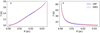 |
Fig. 1 Examples of temperature distributions in cases of externally heated (frame a) and internally heated (frame b) models. The density distribution is that of a 1 M⊙ critically stable Bonnor–Ebert sphere. The blue and dashed red lines show the temperatures calculated with the CRT (Juvela 2005) and DIES programs, respectively. |
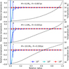 |
Fig. 2 Accuracy of temperature estimates for externally heated models as a function radial position. The frames correspond to 0.2, 1.0, and 10 M⊙ mass models, with the outer radii given in the figure. The dashed black line and the right axis indicate the dust temperatures calculated with 109 photon packages. Compared to this reference solution, the blue, cyan, and red symbols show the results (temperature ratios) for smaller samples of 105, 106, and 108 photon packages. These are plotted for every fifth cell, starting with the centre cell, and adding small shift along the x-axis for better readability. The error bars show the 1σ temperature dispersion based on 100 independent runs. |
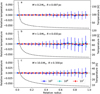 |
Fig. 3 As in Fig. 2 but for models heated by a central source. The results are shown for 105, 106, and 107 photon packages, relative to runs with 108 photon packages. |
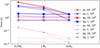 |
Fig. 4 Run times for 106 (transparent colours) and 108 (solid colours) photon packages in the case of the three model clouds with external heating (circles) or internal heating (stars). The solid lines and filled symbols indicate the total run times (including the Python host script) and the dashed lines and open symbols indicate the time of the actual simulation (the OpenCL kernel). |
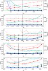 |
Fig. 5 Relative accuracy of temperature estimates in the case of weighted sampling. Each frame corresponds to one of the weighting parameters listed in Table 1. The errors are shown for the surface (blue curves), the half-radius point (green curves), and the centre of the model. The vertical dashed lines mark the default solution without weighting. The dark lines correspond to the 0.2 M⊙ and the light (transparent) curves to the 10 M⊙ models. The cyan lines and the right hand axis show the corresponding run times for the simulation step only. |
3.2 Tests of weighted schemes
Figure 5 shows how weighted sampling affects the precision of the temperature estimates for the externally heated 0.2 M⊙ and 10 M⊙ models. The runs used 107 photon packages, and weighting was applied to only one probability distribution at a time (cf. Table 1).
Biased sampling of the initial package directions with kbg < 0.5 does reduce errors in the model centre. The noise is almost a factor of two lower for kbg = 0.2 (Fig. 5a). This corresponds to almost a factor of four in the run times (for a given noise level), because the run time per photon package remains almost constant. With small values kbg < 0.2, the errors increase in the outer model layers and even exceed those of the innermost shells. The effect kbg is similar for both cloud models, in spite of their different optical depths. Other options of directional weighting have little effect on the noise levels. For the parameter 𝑔E this is natural, because dust remains too cold for the dust re-emission to be of any significance. For the 𝑔S parameter, the errors increase for both large positive and negative parameter values and especially in the model surface layers.
The weighting of the free path of absorptions with kA > 1 was expected to improve the sampling at low densities and thus in the outer parts of the M = 0.2 M⊙ model and more uniformly in the lower-density M = 10 M⊙ model. However, this is not observed in practice, possibly because even the M = 10 M⊙ model is not optically thin. The default unweighted method is in these cases nearly optimal.
Figure 6 shows the corresponding results for the internally heated models. The parameter kbg is omitted because it is not applicable to internal heating. The unweighted DIES calculations are again nearly optimal regarding all four weighting schemes. In the plots, the vertical dashed lines always correspond to the default method without weighting. For most parameters, this is automatically true, and for example when the directions of the background photon packages are weighted with kbg = 0.5, the calculations are identical to the normal, unweighted sampling. However, in the case of scattering directions, the parameter 𝑔S = 0 (isotropic directions of scattered photon packages) does not correspond to the normal run, where the scattering directions are anisotropic due to the dust scattering function. However, for reference, we still include the results from the normal, unweighted run in Fig. 6c by plotting them at the location 𝑔S = 0.
Overall, most weighting schemes of Table 1 are not useful for the examined models. The one exception is the kbg parameter in the case of externally heated models. The relevance of this parameter would increase if the size of the innermost cells were even smaller or if the models were to have a lower optical depth (with fewer scatterings masking the effect of the initial package directions). On the other hand, the weighting methods also did not have a clear effect on the run times. The timing variations are small and affected by random factors, such as the computer power management. Thus, for example, the apparent trend in Fig. 5d in the case of the 0.2 M⊙ model is not reproducible.
The idea of FFI is somewhat similar to the biasing of the free paths, which were not useful in the above models. However, if the optical depths are low enough, these must have a positive effect on the noise levels. We made further comparisons between calculations with the default method (unweighted), a fixed value of kA = 2.5, a density-dependent kA, and the FFI method (Fig. 7). In the density-dependent case, kA(ρ) was set to the value of 3.0 at the lowest densities and to 1.0 (i.e. unmodified free paths) at the highest densities. The parameter was varied linearly as a function of the density logarithm. We used the 10 M⊙ cloud model in this test, but scaled all density values with a constant scaling factor to obtain models of different optical depths. For models similar to or more opaque than the original 10 M⊙ model (i.e. AV> 1.5m), all four alternatives result in similar noise levels (within a factor of two), although the path-length scaling (fixed or variable kA) tends to be poorer than with the default method and FFI is better than the default method. However, at lower optical depths the default method performed the worst and the density-dependent biasing and FFI both reduced the noise significantly, that is, by up to one order of magnitude for the models with the lowest optical depths. The default method and FFI show almost identical run times per photon package, and so this would imply a saving of a factor of almost one hundred in the run time needed to reach a given noise level. The general significance of this is limited by the fact that the highest speed-ups are seen only in very diffuse models. It is also interesting to note that the use of a fixed kA value results in far poorer results than the variable kA(ρ), and this remains true even when other fixed kA values in the range of 1–3 are tested.
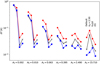 |
Fig. 7 Test of externally heated models of different optical depth, as indicated by the AV values on the x axis. The noise of the temperature estimates is shown for the centre (red symbols, values scaled by 0.1), half radius (black symbols), and outer surface (blue symbols) of the model clouds. For each AV, results are shown (each group of connected symbols, from left to right) for the default method, the use of fixed kA = 2 and density-dependent kA(ρ) parameters, and for the FFI method. |
4 Discussion
The run times of DIES compare favourably for example with the CRT program (Juvela 2005). The codes use different Monte Carlo schemes: DIES uses the IRE and CRT the TMC method. The IRE method is sometimes said to contain no iterations (Bjorkman & Wood 2001), while the traditional method requires that the RT simulation and the temperature updates be iterated until convergence has been reached. However, the difference can also be seen more as a reorganisation of the same of similar calculations. IRE has the advantage that the temperatures are always consistent with the current state of the simulation, although this advantage is offset by the fact that the number of individual temperature updates is higher, which becomes a problem when this entails large costs. Thus, it is still not clear how the IRE method could be implemented efficiently so that also the emission from stochastically heated grains could be estimated.
The performance difference between CRT and DIES is mostly due to the better parallelisation of the latter and especially the possibility of using GPUs for massive parallelisation. The foreseen main use cases of IRE are simple spherical models with a moderate number of cells and a moderate difference between the radii of the smallest cells and the model. Therefore, the tested models also consist only of 100 shells and have a ratio of 1:100 between the smallest cell and the model radius. Whether illuminated only by an internal source or only by an external radiation field, runs with 108 photon packages and run times of ~1 second were enough to determine dust temperatures with an accuracy of δT = 0.1 K. If combined for example with chemical modelling (as mentioned in Sect. 1), such precision is usually sufficient. The errors behaved in a predictable manner, increasing inwards in the externally heated models and outwards in the internally heated ones. If a model includes both types of radiation source, the maximum errors should be even better constrained.
We investigated several possibilities of weighted sampling, but in general did not find these to yield any significant improvement beyond the standard IRE version. Juvela (2005) discussed at least two weighting schemes that were very beneficial in the context of the TMC scheme. The first concerns externally heated models and directions of the photon packages created at the model outer boundary. For radial discretisation ri, the relative projected area of the innermost cells is much smaller  , which leads to a rapid increase in the noise (similar to seen in Fig. 2). Therefore, to reduce the maximum temperature errors, one should send more photon packages that reach the model centre. This works better at low optical depths, when the initial directions of packages are not randomised by scattering. When similar weighting is implemented in DIES, the temperature errors can indeed be decreased almost by a factor of two for a given number of simulated photon packages (for kbg = 0.2, Fig. 5a). This is not yet a very significant improvement for the examined cloud models (Fig. 5a) but could be relevant for models with lower optical depths and larger ratios between the sizes of the smallest cells and the entire model.
In Juvela (2005), the most important weighting scheme for TMC calculations was the location of re-emitted photons. This was crucial when a point source was surrounded by a thin layer of hot dust. Without weighting, the probability of a photon package being created in this layer is proportional to cell volume ( compared to
  for hits by external photons). However, this weighting is only applicable to the TMC scheme, where the positions of the re-emitted photon packages can be created independently. In IRE, re-emission takes place at the location of the absorption events and is directly dictated by the preceding path of the photon packages. However, this also makes the IRE scheme effective in sampling re-emission from hot dust, which might cover only a small fraction of the whole model volume.
The other options of weighted sampling (e.g. direction of emitted or scattered photon packages) were not found to be useful in our tests. In particular, in the case of scattering, the mismatch between the enforced directional distribution and the dust scattering function (usually with 𝑔 ≫ 0) results in a small number of photon packages with large weights, with negative effects (shot noise).
There may also be more general reasons why weighted sampling would be less effective in IRE calculations. One potential factor is the way a photon package is assigned a frequency. In the traditional Monte Carlo, each package has a fixed frequency, and only the weight of the photon package changes as it moves through the model. In contrast, when an IRE package encounters an absorption event, the result is re-emission at a random frequency, which is dictated by the change in the cell emission spectrum (which results from the temperature rise in the cell). One is thus not likely to simulate many consecutive short steps. After the first absorption, re-emission is already at a longer wavelength and with a longer free path. The opposite is also possible. Due to the low optical depth at long wavelengths, a long-wavelength photon package can propagate relatively freely deep into the model. With some probability, it can at re-emission be transformed to a higher frequency, thus also contributing to that part of the local radiation field.
The basic IRE method works well in optically thick models. On the other hand, at low optical depths, the photon packages only rarely interact with the medium, and it can be beneficial to increase the number of interaction events by biasing. The modification of the probability distribution of free paths with a constant factor kA (for modified probability  of free paths) did not perform particularly well, especially compared to a variable and density-dependent modification with kA(ρ). In other words, it seems important that weighting is used only in those parts of the model where it is needed. The density-dependent weighting with kA(ρ) still requires that we set parameters, how much weighting is applied, and how that depends on the density. Although the results were good in the test cases, the same parameter values might not work well in other cases and might need to be tuned separately. Therefore, FFI appears to be a good alternative; it performed almost as well as the density-dependent weighting for optically thin models, and even slightly better for the optically thick models, and has no free parameters. The method requires some additional computations, but the overheads are barely visible in our tests.
There are still other techniques that might improve the efficiency of IRE calculations, at least for certain types of models. One such method is photon splitting, which could enhance the radiation field sampling in selected parts of the model. However, this would be slightly more difficult to implement efficiently, especially on GPUs, where the goal is to have all the threads always performing strictly the same operations. We also did not consider the frequency distribution of the re-emitted photon packages. Weighted frequency sampling may not improve the accuracy of temperature estimates but, for example, could be helpful to produce better estimates of scattered light in given frequency bands. However, due to its use of a fixed grid of frequencies, the TMC method appears better suited for the generation of images of scattered light.
Although we have examined only spherically symmetric models in this paper, all the discussed methods can in principle be used in three-dimensional RT calculations. In any model, it is important to consider which directions or regions should be emphasised with the weighted sampling.
Finally, we note that there is one small difference between TMC and IRE that could lead to differences in their results. In the IRE method, re-emission takes place at the locations where photon packages are absorbed, whereas in TMC this happens uniformly over the cell. This affects the fraction of re-emission that is subsequently reabsorbed in the same cell or transported to the next cells. In this respect, the IRE way is more correct; although, since each cell is still assigned only a single temperature, neither method can actually resolve differences at subcell scales. We tested this by modifying IRE so that the position of re-emission was randomised within the cell volume. No visible differences were observed for any of the models examined in this paper. However, with sufficiently high optical depths and sufficiently coarse discretisation, the difference could become noticeable, although the actual errors would probably still be dominated directly by the poor discretisation.
5 Conclusions
We present DIES, a parallel implementation of the IRE method for dust RT calculations. Here we use the program to study the potential benefits of weighted sampling. This work led to the following conclusions:
IRE is also well suited for GPU computing. For one-dimensional models of moderate size (~ 100 shells), the RT calculations could be completed within a few seconds, with temperature uncertainties being sufficiently low for most applications (δT ≲ 0.1 K);
Weighted sampling is usually not needed for models of high or moderate optical depth. In particular, in case of embedded point sources, the IRE method itself already provides efficient sampling of the dust re-emission, even when this is confined to a very small volume;
There can be some advantage from biasing the directions of the photon packages representing the external radiation field. This is true especially for optically thin models and when the projected area of the innermost model cells is very small;
The IRE method samples absorptions only at discrete positions, which can result in larger temperature errors in optically thin models. The FFI technique (i.e. forcing at least one interaction for each photon package) is a simple way to reduce the noise. Density-dependent biasing of the photon free paths can be equally beneficial but requires some tuning of the method parameters.
Acknowledgements
MJ acknowledges the support of the Research Council of Finland Grant No. 348342.
Appendix A Comparison to CRT program
We compared the run times of DIES to those of the CRT program (Juvela 2005). The chosen model clouds is a 1 M⊙ Bonnor-Ebert sphere that has been divided into 100 concentric shells of equal thickness. The model is illuminated either only by an external isotropic radiation field or by a central point source, as described in Sect. 3. The runs were performed on the same laptop, CRT runs using the CPU and DIES the laptop GPU.
Figure A.1 shows the results for the externally heated model. The dust temperatures are low, re-emission is insignificant, and therefore CRT runs require only one iteration. Plot also shows results for alternative runs with weighted sampling, where photon packages were targeted preferentially towards the model centre. This has a small but noticeable effect in decreasing the noise in the innermost shells. The number of photon packages was selected so that the run times (CRT on CPU and DIES on GPU) were approximately similar. The resulting noise of the DIES estimates is more than a factor of two lower in the outer part of the model, thus in theory corresponding to a factor of four saving in the run time. However, in the centre the noise levels are identical. We suspect that CRT benefits here from the fact that all frequencies are sampled equally with the same number of photon packages. In contrast, DIES creates photon packages according to the spectrum of the background radiation. This gives more emphasis for the frequencies near the peak of the emission spectrum, while dust in the model centre is heated mainly by direct background radiation at somewhat longer wavelengths. This suggest that one should consider weighting the sampling also as a function of the frequency, especially in case of optically very thick models. As mentioned above, re-emission plays no role in the case of the externally heated model.
Figure A.2 shows a similar comparison when the model cloud is heated only by a central radiation source. The basic IRE method already samples the re-emission well, and there is no need for weighted sampling. In contrast, CRT shows in the unweighted case large noise and very strong bias. This is because, when the re-emission is sampled uniformly over the model volume, only few photon packages are created in the hot shells near the central radiation source. However, weighted sampling reduces the CRT noise by two orders of magnitude. In this case the weighting means that the same number of re-emitted photon packages were created for each shell, irrespective of their volumes (cf. Juvela 2005). The quoted CRT run times are for two iterations. The first iteration gives initial estimates for the dust temperatures, and only the second iteration gives the first indication of how these are affected by re-emission. However, several more iterations would be needed to reach final convergence in this test case, and the real cost of CRT calculations would be a few times higher than indicated in the figure. This remains true, even though in multi-iteration runs the number of photon packages per iteration could be decreased with the help of a reference field, as discussed in Juvela (2005). Thus, the IRE method is simpler and likely to be much more efficient when the model includes strong local heating. However, the methods are also seen to prioritise different parts of the model. IRE is more accurate in the inner regions, while the standard Monte Carlo simulation could still in some cases be superior in the outer parts.
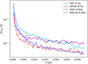 |
Fig. A.1 Noise of dust temperature estimates, δT, as a function of the radius in an externally heated 1 M⊙ model cloud. Results are shown for the CRT program (solid lines) and the DIES program (dashed lines), with the run times quoted in the legend. Results are shown also for weighted runs, when photon packages are targeted more towards the model centre (“CRT-W“ and “DIES-W”, respectively). The noise has been estimated from the standard deviation between 50 runs. |
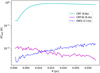 |
Fig. A.2 As Fig. A.1 but for a model with a central radiation source and no external radiation field. |
References
- Baes, M., Gordon, K. D., Lunttila, T., et al. 2016, A&A, 590, A55 [NASA ADS] [CrossRef] [EDP Sciences] [Google Scholar]
- Bjorkman, J. E., & Wood, K. 2001, ApJ, 554, 615 [NASA ADS] [CrossRef] [Google Scholar]
- Black, J. H., & van Dishoeck, E. F. 1987, ApJ, 322, 412 [Google Scholar]
- Bonnor, W. B. 1956, MNRAS, 116, 351 [NASA ADS] [CrossRef] [Google Scholar]
- Camps, P., & Baes, M. 2018, ApJ, 861, 80 [NASA ADS] [CrossRef] [Google Scholar]
- Camps, P., Misselt, K., Bianchi, S., et al. 2015, A&A, 580, A87 [NASA ADS] [CrossRef] [EDP Sciences] [Google Scholar]
- Chen, L.-F., Chang, Q., Wang, Y., & Li, D. 2022, MNRAS, 516, 4627 [NASA ADS] [CrossRef] [Google Scholar]
- Compiègne, M., Verstraete, L., Jones, A., et al. 2011, A&A, 525, A103 [Google Scholar]
- Desert, F. X., Boulanger, F., & Shore, S. N. 1986, A&A, 160, 295 [NASA ADS] [Google Scholar]
- Draine, B. T. 2003, ARA&A, 41, 241 [NASA ADS] [CrossRef] [Google Scholar]
- Draine, B. T., & Li, A. 2001, ApJ, 551, 807 [NASA ADS] [CrossRef] [Google Scholar]
- Ebert, R. 1955, Z. Astrophys., 37, 217 [NASA ADS] [Google Scholar]
- Gordon, K. D., Baes, M., Bianchi, S., et al. 2017, A&A, 603, A114 [NASA ADS] [CrossRef] [EDP Sciences] [Google Scholar]
- Henyey, L. G., & Greenstein, J. L. 1941, ApJ, 93, 70 [Google Scholar]
- Juvela, M. 2005, A&A, 440, 531 [NASA ADS] [CrossRef] [EDP Sciences] [Google Scholar]
- Kahan, W. 1965, Commun. ACM, 8, 40 [Google Scholar]
- Krieger, A., & Wolf, S. 2023, A&A, 680, A67 [NASA ADS] [CrossRef] [EDP Sciences] [Google Scholar]
- Krieger, A., & Wolf, S. 2024, A&A, 682, A99 [NASA ADS] [CrossRef] [EDP Sciences] [Google Scholar]
- Li, A., & Draine, B. T. 2001, ApJ, 554, 778 [Google Scholar]
- Lucy, L. B. 1999, A&A, 344, 282 [NASA ADS] [Google Scholar]
- Mattila, K. 1970, A&A, 9, 53 [NASA ADS] [Google Scholar]
- Sipilä, O., Zhao, B., & Caselli, P. 2020, A&A, 640, A94 [NASA ADS] [CrossRef] [EDP Sciences] [Google Scholar]
- Steinacker, J., Baes, M., & Gordon, K. D. 2013, ARA&A, 51, 63 [CrossRef] [Google Scholar]
- Witt, A. N. 1977, ApJS, 35, 1 [NASA ADS] [CrossRef] [Google Scholar]
Available at https://github.com/mjuvela/ISM
All Tables
All Figures
|
Fig. 1 Examples of temperature distributions in cases of externally heated (frame a) and internally heated (frame b) models. The density distribution is that of a 1 M⊙ critically stable Bonnor–Ebert sphere. The blue and dashed red lines show the temperatures calculated with the CRT (Juvela 2005) and DIES programs, respectively. |
| In the text | |
|
Fig. 2 Accuracy of temperature estimates for externally heated models as a function radial position. The frames correspond to 0.2, 1.0, and 10 M⊙ mass models, with the outer radii given in the figure. The dashed black line and the right axis indicate the dust temperatures calculated with 109 photon packages. Compared to this reference solution, the blue, cyan, and red symbols show the results (temperature ratios) for smaller samples of 105, 106, and 108 photon packages. These are plotted for every fifth cell, starting with the centre cell, and adding small shift along the x-axis for better readability. The error bars show the 1σ temperature dispersion based on 100 independent runs. |
| In the text | |
|
Fig. 3 As in Fig. 2 but for models heated by a central source. The results are shown for 105, 106, and 107 photon packages, relative to runs with 108 photon packages. |
| In the text | |
|
Fig. 4 Run times for 106 (transparent colours) and 108 (solid colours) photon packages in the case of the three model clouds with external heating (circles) or internal heating (stars). The solid lines and filled symbols indicate the total run times (including the Python host script) and the dashed lines and open symbols indicate the time of the actual simulation (the OpenCL kernel). |
| In the text | |
|
Fig. 5 Relative accuracy of temperature estimates in the case of weighted sampling. Each frame corresponds to one of the weighting parameters listed in Table 1. The errors are shown for the surface (blue curves), the half-radius point (green curves), and the centre of the model. The vertical dashed lines mark the default solution without weighting. The dark lines correspond to the 0.2 M⊙ and the light (transparent) curves to the 10 M⊙ models. The cyan lines and the right hand axis show the corresponding run times for the simulation step only. |
| In the text | |
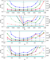 |
Fig. 6 As in Fig. 5 but for the internally heated models. |
| In the text | |
|
Fig. 7 Test of externally heated models of different optical depth, as indicated by the AV values on the x axis. The noise of the temperature estimates is shown for the centre (red symbols, values scaled by 0.1), half radius (black symbols), and outer surface (blue symbols) of the model clouds. For each AV, results are shown (each group of connected symbols, from left to right) for the default method, the use of fixed kA = 2 and density-dependent kA(ρ) parameters, and for the FFI method. |
| In the text | |
|
Fig. A.1 Noise of dust temperature estimates, δT, as a function of the radius in an externally heated 1 M⊙ model cloud. Results are shown for the CRT program (solid lines) and the DIES program (dashed lines), with the run times quoted in the legend. Results are shown also for weighted runs, when photon packages are targeted more towards the model centre (“CRT-W“ and “DIES-W”, respectively). The noise has been estimated from the standard deviation between 50 runs. |
| In the text | |
|
Fig. A.2 As Fig. A.1 but for a model with a central radiation source and no external radiation field. |
| In the text | |
Current usage metrics show cumulative count of Article Views (full-text article views including HTML views, PDF and ePub downloads, according to the available data) and Abstracts Views on Vision4Press platform.
Data correspond to usage on the plateform after 2015. The current usage metrics is available 48-96 hours after online publication and is updated daily on week days.
Initial download of the metrics may take a while.