| Issue |
A&A
Volume 689, September 2024
|
|
|---|---|---|
| Article Number | A36 | |
| Number of page(s) | 11 | |
| Section | Stellar structure and evolution | |
| DOI | https://doi.org/10.1051/0004-6361/202450543 | |
| Published online | 30 August 2024 | |
A conclusive non-detection of magnetic field in the Am star o Peg with high-precision near-infrared spectroscopy⋆
1
Department of Physics and Astronomy, Uppsala University, Box 516 75120 Uppsala, Sweden
2
Institut de Recherche en Astrophysique et Planétologie, Université de Toulouse, CNRS, IRAP/UMR 5277, 14 Avenue Edouard Belin, 31400 Toulouse, France
3
Institut für Astrophysik und Geophysik, Georg-August-Universität, Friedrich-Hund-Platz 1, 37077 Göttingen, Germany
4
Thüringer Landessternwarte Tautenburg, Sternwarte 5, 07778 Tautenburg, Germany
5
Department of Astronomy, University of Geneva, Chemin Pegasi 51, 1290 Versoix, Switzerland
6
Max-Planck-Institut für Sonnensystemforschung, Justus-von-Liebig-Weg 3, 37077 Göttingen, Germany
7
European Southern Observatory, Karl-Schwarzschild-Str. 2, 85748 Garching bei München, Germany
8
Instituto de Astrofísica de Andalucía – CSIC, Glorieta de la Astronomía s/n, 18008 Granada, Spain
Received:
29
April
2024
Accepted:
21
May
2024
Context. The A-type metallic-line (Am) stars are typically considered to be non-magnetic or to possess very weak sub-G magnetic fields. This view has been repeatedly challenged in the literature; most commonly for the bright hot Am star o Peg. Several studies claim to have detected 1–2 kG field of unknown topology in this object, possibly indicating a new process of magnetic-field generation in intermediate-mass stars.
Aims. In this study, we revisit the evidence of a strong magnetic field in o Peg using new high-resolution spectropolarimetric observations and advanced spectral fitting techniques.
Methods. We estimated the mean magnetic field strength in o Peg from the high-precision CRyogenic InfraRed Echelle Spectrograph (CRIRES+) measurement of near-infrared (NIR) sulphur lines. We modelled this observation with a polarised radiative transfer code, including treatment of the departures from local thermodynamic equilibrium. In addition, we used the least-squares deconvolution multi-line technique to derive longitudinal field measurements from archival optical spectropolarimetric observations of this star.
Results. Our analysis of the NIR S I lines reveals no evidence of Zeeman broadening, ruling out magnetic field with a strength exceeding 260 G. This null result is compatible with the relative intensification of Fe II lines in the optical spectrum, taking into account blending and uncertain atomic parameters of the relevant diagnostic transitions. Longitudinal field measurements on three different nights also yield null results with a precision of 2 G.
Conclusions. This study refutes the claims of kG-strength dipolar or tangled magnetic field in o Peg. This star therefore appears to be non-magnetic, with surface magnetic field characteristics no different from those of other Am stars.
Key words: stars: chemically peculiar / stars: early-type / stars: magnetic field / stars: individual: o Peg
© The Authors 2024
 Open Access article, published by EDP Sciences, under the terms of the Creative Commons Attribution License (https://creativecommons.org/licenses/by/4.0), which permits unrestricted use, distribution, and reproduction in any medium, provided the original work is properly cited.
This article is published in open access under the Subscribe to Open model. Subscribe to A&A to support open access publication.
1. Introduction
The upper main sequence stars, with spectral classes from early B to early F, can be separated into two distinct groups according to the characteristics of their surface magnetic field (Preston 1974; Donati & Landstreet 2009). One group, the so-called magnetic chemically peculiar (mCP) or Ap/Bp stars, exhibit stable, globally organised kG-strength fields on their surfaces. These objects comprise about 10% of all intermediate-mass and massive stars (Grunhut et al. 2017; Schöller et al. 2017; Sikora et al. 2019). Another, more sizeable, group includes normal and non-magnetic chemically peculiar stars, which show no evidence of strong organised surface magnetic fields. The cool end of the temperature sequence of non-magnetic CP stars is populated by the metallic-line A-type (Am) stars. These stars are known for their slow rotation, common membership in close binary systems, a moderate overabundance of iron-peak elements, and an underabundance of Ca and Sc (e.g. Ghazaryan et al. 2018). The brightest star in the sky, Sirius, is an example of a hot Am star (Landstreet 2011; Cowley et al. 2016).
The spectroscopic characteristics of Am stars facilitate precise measurements of the mean longitudinal magnetic field, ⟨Bz⟩, using high-resolution circular polarisation observations (Wade et al. 2000). Applications of this technique, which is only sensitive to a global magnetic field component, ruled out the presence of ≳10 G large-scale fields in Am stars (Shorlin et al. 2002; Aurière et al. 2010). This upper limit is at least one order of magnitude below the ∼100 G weak-field limit of mCP stars (Aurière et al. 2007; Kochukhov et al. 2023a). The observational characterisation of Am-star magnetism is more nuanced for weaker fields. Definitive ⟨Bz⟩ measurements at a level of 5–10 G, compatible with a global dipolar-like field sheared by a differential rotation, were reported for at least one Am star, γ Gem (Blazère et al. 2020). At the same time, circular polarisation signatures corresponding to sub-G magnetic fields have been detected in several bright Am stars (Petit et al. 2011; Blazère et al. 2016; Neiner et al. 2017). Considering the conspicuous gap in the magnetic-field-strength distribution between Am and mCP stars, and the different geometrical characteristics of their fields, the ultraweak Am-star magnetism likely has a different physical origin compared to stable fossil fields found in mCP stars (Cantiello & Braithwaite 2019; Jermyn & Cantiello 2020).
The view that Am stars are either non-magnetic or host only very weak fields is occasionally challenged in the literature. The star o Peg (43 Peg, HR 8641, HD 214994) is at the centre of this debate. This is a bright, narrow-line hot Am star frequently targeted by detailed chemical abundance and model atmosphere analyses based on high-resolution optical (Adelman 1988; Landstreet et al. 2009; Takeda et al. 2012; Adelman et al. 2015) and ultraviolet (Adelman et al. 1993) spectra. No longitudinal magnetic field was detected in this star by Shorlin et al. (2002). Their single magnetic field measurement, ⟨Bz⟩ = −32 ± 20 G, is compatible with zero, albeit at an inferior precision relative to what has been achieved for similarly bright stars in more recent studies. On the other hand, Mathys & Lanz (1990) reported the presence of a ≈2 kG mean magnetic field, ⟨B⟩, in o Peg based on a statistical line-width analysis and an empirical relation between ⟨B⟩ and the relative equivalent widths of the Fe II 614.7 and 614.9 nm lines. Takeda (1991) studied the behaviour of this line pair in a magnetic field using radiative transfer calculations, confirming ∼2–3 kG magnetic field in o Peg. Subsequently, Takeda (1993) measured a ∼2 kG field by minimising the scatter of abundances derived from lines of different strength. These results were recently revised by Takeda (2023), who analysed new high-quality spectroscopic observations of o Peg with several of the aforementioned techniques and concluded, once again, that o Peg exhibits a mean magnetic field of ⟨B⟩≈1–2 kG.
The vast discrepancy between the ∼kG field strength inferred from the Stokes I spectra and the ∼50 G upper limit obtained from Stokes V observations is usually interpreted in a context where it is assumed that the putative field of o Peg is ‘complex’ or ‘tangled’, meaning that it is dominated by a small-scale component that produces broadening and intensification of line profiles in the Stokes I spectra but remains undetectable in Stokes V due to cancellation of the contributions of the surface regions with different field polarities to the disc-integrated stellar polarisation spectra. This situation is often found in cool active stars with dynamo fields (e.g. Kochukhov et al. 2020, 2023b; Kochukhov 2021), although the ratio ⟨B⟩/⟨Bz⟩∼100 implied by the previous magnetic field studies o Peg appears to be exceptionally large even compared to cool stars. Contrary to this picture, Takeda (2023) postulated that o Peg has a global dipolar magnetic field viewed from the magnetic equator, implying that the null ⟨Bz⟩ measurement by Shorlin et al. (2002) is explained by a fortuitous cancellation of the signals from the positive and negative magnetic hemispheres.
This series of seemingly consistent magnetic field determinations for o Peg is having a noticeable influence on the community’s understanding of Am stars in general. The work by Mathys & Lanz (1990) is frequently cited in review papers (Landstreet 1992; Dworetsky 1993; Smith 1996; Kurtz & Martinez 2000; Mathys 2004a,b, 2009; Hubrig & Schöller 2021), and has inspired applications of the same magnetic field measurement procedures to other Am stars (Lanz & Mathys 1993; Savanov 1994; Scholz et al. 1997), to their hotter counterparts, HgMn stars (Takada-Hidai & Jugaku 1992; Hubrig & Castelli 2001; Kochukhov et al. 2013), and to other A-type stars (Takada-Hidai & Jugaku 1993). In a wider context, some authors consider the presumed complex and strong magnetic field of o Peg to be representative of all Am stars (e.g. Drake et al. 1994). However, the majority of studies adopt a more conservative viewpoint that this star is, for some reason, exceptional in terms of its magnetic characteristics (Debernardi et al. 2000; Hui-Bon-Hoa 2000; Carrier et al. 2002; Korčáková et al. 2022).
In the present study, we revisit the question of whether or not o Peg is a magnetic star. To this end, we use new spectropolarimetric measurements to characterise the global magnetic field component at a far greater precision than in previous studies. Moreover, we investigate the Zeeman effect using high signal-to-noise (S/N) optical and – for the first time for any Am star – high-resolution near-infrared (NIR) spectra. The paper is structured as follows. We start with an overview of the observational data employed in this study (Sect. 2). We proceed to describe our polarised spectrum synthesis methodology in Sect. 3, including assessment of the deviations from local thermodynamic equilibrium (LTE) and partial Paschen-Back (PPB) splitting. Subsequently, we present our analysis of NIR (Sect. 4) and optical (Sect. 5) profiles of magnetically sensitive lines, leading to a new sensitive upper limit on the total magnetic field strength of o Peg. We complement this analysis with high-precision spectropolarimetric measurements of the longitudinal field (Sect. 6) and derivation of an upper limit of the dipolar magnetic component compatible with these observations. The paper is concluded with a discussion and a summary of our findings in Sect. 7.
2. Observations
2.1. Near-infrared spectroscopy
We observed o Peg on August 12, 2023, with the upgraded CRyogenic InfraRed Echelle Spectrograph (CRIRES+, Dorn et al. 2023) at the European Southern Observatory (ESO) Very Large Telescope (VLT) located on Cerro Paranal, Chile. CRIRES+ is a high-resolution (R ≈ 105) cross-dispersed NIR spectropolarimeter mounted on a Nasmyth focus of the 8m Unit Telescope 3 at the VLT. Our observations were carried out as part of the CRIRES+ consortium guaranteed time observations.
The instrument was setup with a slit width of 0.2 arcsec, and we obtained observations in four standard wavelength settings: Y1029, J1228, H1567, and H1582. For observations in each wavelength setting, we obtained eight individual exposures with a 30s integration time, taken with an AAAABBBB nodding pattern. The nodding procedure consists in placing the star on two distinct positions (A and B) on the slit and facilitates the removal of sky background and detector artefacts in the data reduction. The log of our CRIRES+ observations of o Peg is presented in Table 1.
Log of CRIRES+ observations of o Peg.
To reduce the data, we used the CRIRES+ data reduction pipeline cr2res (Dorn et al. 2023). First, we reduced the raw calibration frames association with our programme taken as part of the daily calibration routine. These data consist of dark, flat field, and wavelength calibration frames (Fabry-Perot etalon, Uranium-Neon lamp) and were reduced using the standard calibration reduction cascade as laid out in the cr2res pipeline user manual1.
We then reduced the science data for each wavelength setting using the cr2res_obs_nodding recipe. This recipe applies the reduced calibrations to the science raw frames (bad pixel mask, pixel-to-pixel sensitivity), substracts the B frames from the A frames, extracts the 1D science and error spectra for the two nodding positions using an optimal extraction algorithm, and applies the wavelength solution to the spectra.
The analysis presented below (Sect. 4) focuses on the S I lines at 1046 nm observed in the Y1029 setting. The S/N reached at this wavelength is around 480 according to the formal error propagation by the cr2res pipeline. This agrees with the empirical measurement of the standard deviation of continuum points in the vicinity of the S I lines.
2.2. Optical spectroscopy
Considering the particular importance and common usage of the Fe II 614.7–614.9 nm line pair for measuring magnetic fields in chemically peculiar stars, including o Peg, we revisit this magnetic diagnostic in Sect. 5. At the same time, we refrain from reassessing all types of magnetic detection methods applied to o Peg and similar stars based on Stokes I profiles of optical lines because the NIR magnetic diagnostic technique developed in the present paper (Sect. 4) is far superior in terms of its ability to detect magnetic fields.
Among multiple optical archival spectra of o Peg covering this line pair, we chose to use the observed spectrum published by Takeda (2023) due to its higher resolution and higher S/N. This spectrum was constructed from a series of individual observations obtained over several nights in October 2008 using the HIDES coudé echelle spectrograph at the 1.88 m telescope of the Okayama Astrophysical Observatory. The spectrum has a resolving power of λ/Δλ ≈ 105 and a very high S/N approaching 1000. Further details of the acquisition and reduction of these data can be found in Takeda et al. (2012) and Takeda (2023).
2.3. Optical spectropolarimetry
Three previously unpublished circular polarisation observations of o Peg are included in the PolarBase archive (Petit et al. 2014). These spectra were obtained on three non-consecutive nights between June 10 and June 19, 2014, with the ESPaDOnS spectropolarimeter (Donati et al. 2006) installed at the 3.6 m Canada-France-Hawaii telescope. For each observation, the intensity (Stokes I) and circular polarisation (Stokes V) spectra were recorded using a sequence of four 110 s subexposures, resulting in a peak S/N of 940–970 per pixel of the extracted intensity spectrum at λ = 520 nm. The individual times of mid-exposure and S/N values are provided in Table 2.
Mean longitudinal magnetic field measurements derived from the ESPaDOnS observations.
The ESPaDOnS spectra have a fixed format that covers the 370–1030 nm wavelength range with 40 partially overlapping echelle orders at a resolving power of λ/Δλ = 65 000. The o Peg observations were reduced by the Libre-ESpRIT pipeline (Donati et al. 1997) running at the telescope. We post-processed the spectra with the help of the procedures described in Rosén et al. (2018) to improve continuum normalisation. In this study, the ESPaDOnS circular polarisation observations are employed to obtain new measurements of the mean longitudinal magnetic field and derive constraints on the global magnetic field geometry in Sect. 6.
3. Modelling methodology
3.1. Polarised spectrum synthesis
The spectrum synthesis modelling carried out in this paper is based on the polarised radiative transfer code Synmast (Kochukhov 2007; Kochukhov et al. 2010). This software derives a numerical solution of the polarised radiative transfer equation for a given model atmosphere, limb angle, and local magnetic field vector. Synmast shares the equation-of-state module with the Spectroscopy Made Easy (SME) package (Piskunov & Valenti 2017) and has been extensively tested against independent polarised radiative transfer codes (Wade et al. 2001).
In the calculations for the present paper, we adopted a simplified model of stellar magnetic field comprised of a uniform radial field distribution. This approach, widely used in modelling Zeeman broadening and intensification effects in the Stokes I spectra of active stars (e.g. Lavail et al. 2019; Kochukhov et al. 2020; Hahlin et al. 2023), requires calculation of a small number (typically seven) of local intensity spectra at different limb angles to obtain accurate disc-integrated profiles. As the radial field is seen from different aspect angles depending on the centre-to-limb position, its cumulative effect on the Zeeman split line profiles is more representative of a possible complex magnetic configuration than any field geometry defined relative to the observer’s line of sight (e.g. a purely transverse or purely longitudinal field). In fact, the disc-integrated Stokes I line profiles corresponding to a uniform radial magnetic field turn out to be very similar to those calculated for a star covered by an anisotropic randomly oriented field with the same strength. Therefore, our model is compatible with the hypothesis of a complex tangled magnetic field, as explored by some previous studies of o Peg.
The model atmosphere employed in the present study was calculated with the LLmodels code (Shulyak et al. 2004) assuming an effective temperature of Teff = 9500 K, a surface gravity of log g = 3.6, and a microturbulent velocity of ξt = 2 km s−1. These are typical atmospheric parameter values inferred by modern detailed spectroscopic studies of o Peg (see the summary in Takeda 2023). For these model atmosphere calculations, we used individual chemical abundances of o Peg from Adelman et al. (2015).
It is not obvious which spectral lines are best suited for accurate magnetic field measurements in Stokes I in the available wide-wavelength-coverage optical and NIR spectra of o Peg. In particular, spectral lines with the largest effective Landé factors are not necessarily the most informative diagnostics of weaker magnetic fields because subtle Zeeman broadening effects are often washed out by rotational broadening. As shown by several studies of cool active stars (e.g. Kochukhov & Lavail 2017; Kochukhov et al. 2020, 2023b), spectral lines with above-average effective Landé factors and complex Zeeman splitting patterns may provide useful alternative diagnostics owing to their strong magnetic intensification response. To identify the most suitable magnetically sensitive lines, we modelled the entire optical and NIR spectrum of o Peg with Synmast, comparing non-magnetic calculations with the theoretical spectra corresponding to B = 1 and 2 kG. After applying the appropriate rotational and instrumental broadening, the S I triplet at 1045.5–1045.9 nm has emerged as the most promising diagnostic feature in the NIR wavelength region. The three components of this multiplet are well separated for the projected equatorial velocity (ve sin i) of o Peg and exhibit distinct magnetic responses due to different effective Landé factors (ranging from 1.25 to 2.00) and diverse Zeeman splitting patterns. The relevant line parameters of the S I triplet are summarised in Table 3, where we note that the absolute oscillator strengths of the three lines are measured with uncertainties of the order of 0.01 dex (Zerne et al. 1997). There are no significant blending contributions to any of these three lines for the effective temperature and chemical abundance of o Peg.
Atomic line data adopted for the S I NIR triplet.
Figure 1a illustrates a series of Synmast calculations of the S I triplet with increasing magnetic field strength. These spectra are convolved with the projected rotational velocity ve sin i = 5.9 km s−1, macroturbulent velocity ζt = 3.7 km s−1 (similar to the results obtained in Sect. 4), and a Gaussian instrumental profile corresponding to R = 105 to represent instrumental broadening of our CRIRES+ spectrum. The effect of magnetic field is already apparent at B ≈ 1 kG, with the S I 1045.5 nm line exhibiting less excess magnetic broadening compared to the 1045.9 and, in particular, the 1045.7 nm line. The latter feature starts showing partially resolved Zeeman splitting at B ≈ 2 kG. This diverse magnetic response of lines of the same multiplet (or more generally of nearby lines of the same ion with similar excitation potentials and precise relative oscillator strengths) is ideal for disentangling magnetic broadening and intensification from competing broadening effects due to turbulent and rotational velocity fields. No other spectral lines with a diagnostic potential comparable to the S I triplet were found in our calculations for the CRIRES+ wavelength region. Hence, we restricted the NIR part of our study to these S I lines. At the same time, we re-examined the Fe II 614.7–614.9 nm lines based on previously published observations (see Sect. 2.2) to address claims of magnetic field detections using this line pair.
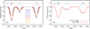 |
Fig. 1. Behaviour of the NIR S I triplet in magnetic field. (a) Synthetic Zeeman profiles for different magnetic field strengths. The corresponding splitting patterns are shown schematically above each line for B = 3 kG. (b) Comparison of the Zeeman (black dashed line) and PPB (red solid line) calculations for B = 3 kG. The splitting patterns above the line profiles are illustrated for the PPB case. |
3.2. Non-local thermodynamic equilibrium effects
In order to take full advantage of the diagnostic power of the S I 1046 nm triplet, departures from local thermodynamic equilibrium (LTE) must be taken into account. Previous studies of non-LTE effects for sulphur include theoretical investigations by Takeda et al. (2005) and Korotin (2009), and applications mainly to the Sun (e.g. Scott et al. 2015) and other FGK-type stars (e.g. Nissen et al. 2007; Caffau et al. 2016), with fewer studies of warm stars (e.g. Kamp et al. 2001). All these studies point to significant effects for the neutral atom.
For this work, we carried out our own non-LTE calculations for sulphur. The statistical equilibrium was solved for using Balder (Amarsi et al. 2018b, 2022). The departure coefficients generated by Balder were read into Synmast and used to correct the LTE line opacity and source function prior to spectrum synthesis, as described in Piskunov & Valenti (2017). Balder is based on Multi3D (Leenaarts & Carlsson 2009) but with several modifications, the most important for the present work being related to the equation of state and background opacities (calculated with Blue; Zhou et al. 2023). Rayleigh scattering in the UV was considered for hydrogen (Lee & Kim 2004) and helium (Langhoff et al. 1974), while other background transitions were treated in pure absorption.
The model atom we use here was also used in Carlos et al. (2024) and will be described in a future paper (Amarsi et al., in prep.). Briefly, it contains 66 levels in total (including seven ‘superlevels’ of neutral sulphur, and four levels of ionised sulphur). Radiative transition data come from the National Institute of Standards and Technology (NIST, Kramida et al. 2022), and are based on the calculations of Zatsarinny & Bartschat (2006); and from the Opacity Project (e.g. Seaton et al. 1992). Electron collision data come from empirical recipes (van Regemorter 1962; Allen 1973). Hydrogen collisions were taken from Belyaev & Voronov (2020) and combined with data calculated using the recipe of Kaulakys (1991) in the scattering-length approximation (see Barklem 2016 and Amarsi et al. 2018a). Pressure broadening by electrons and by neutral hydrogen was taken into account based on data from the Kurucz database (e.g. Kurucz 1995) and by interpolating tables of hydrogen collisional cross-section data (Anstee & O’Mara 1995; Barklem & O’Mara 1997; Barklem et al. 1998).
The statistical equilibrium calculations were performed on the same LLmodels atmosphere used for the analysis described in Sect. 4. The microturbulent velocity ξt was fixed at 2.0 km s−1, which is close to the best-fitting result for o Peg (see Sect. 4). Assuming sulphur to be a trace element with no impact on the model atmosphere, the calculations were performed for a range of abundances: log NS/Ntot = −4.60 to −4.25 (log NS/NH + 12 = 7.42 to 7.77), with a step size of 0.05 dex.
The different components of the S I triplet are affected differently by departures from LTE, as seen in Fig. 2. At the best-fitting parameters of o Peg, the strength of the weakest, middle component is quite close to that in LTE, while the stronger blue and red components are significantly stronger in non-LTE. These effects can be understood from Fig. 3, which shows the departure coefficients of the lower and upper terms at the best-fitting abundance as a function of logarithmic Rosseland-mean optical depth log τRoss. To first order, the line opacity scales with the departure coefficient of the lower level bl, while the line source function is proportional to the ratio of the upper and lower level departure coefficients bu/bl (e.g. Rutten 2003). The dip in bl and bu in deeper layers, log τRoss ≈ −0.6, is caused by pumping due to absorption of UV photons in bound-free transitions (overionisation), resulting primarily in lower line opacity and a weakening of lines forming in this region. Towards higher layers, photon losses from high-lying transitions become significant. In particular, the S I triplet itself strongly regulates the populations of its levels, such that bl rises and bu/bl falls: they pass through unity at around log τRoss ≈ −1.4.
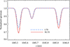 |
Fig. 2. Impact of departures from LTE on the synthetic profiles of the NIR S I triplet. These calculations were carried out for B = 0 kG, log NS/Ntot = −4.35, ξt = 2 km s−1, and other parameters of o Peg set to the best-fitting values found in Sect. 4. |
The different effects on the three components are directly related to their different formation depths. This is because the model atom adopts efficient collisional coupling between the fine structure levels (e.g. Lind & Amarsi 2024), and so the departure coefficients are identical for the three components. The formation depths can be quantified via the contribution function to the depression in the disc-integrated flux (e.g. Albrow & Cottrell 1996; Amarsi 2015); these functions calculated at line centre are overplotted in Fig. 3. The stronger blue and red components mostly form in layers with log τRoss ≲ −1.4, where bl > 1 and bu/bl < 1: the line opacity is increased relative to LTE and the line source function is reduced relative to LTE, and both act to increase the line strength. In contrast, the weakest middle component forms in deeper layers, where it suffers from both line strengthening and line weakening effects. Consequently, the broadened line profile appears closer to that predicted in LTE.
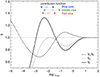 |
Fig. 3. Departure coefficients of the lower and upper levels of the S I triplet, bl and bu, respectively. Their ratio is also shown. The full-width at half maximum (arrows) and peak depth (open circles) of the contribution functions to the depression in the disc-integrated flux – calculated at line centre – are shown for the three lines of the S I triplet. |
3.3. Partial Paschen-Back splitting
With the separation of the lower energy levels of ≈4 cm−1, the magnetic splitting of the Fe II 614.7–614.9 nm line pair studied in Sect. 5 is affected by the PPB effect (Mathys 1990). This phenomenon arises when the magnetic splitting of the atomic energy levels becomes comparable to the fine-structure splitting, resulting in asymmetric line splitting patterns. For lines forming in the PPB regime, both positions and strengths of the Zeeman components exhibit a complex non-linear behaviour with the magnetic field strength. However, deviation from the linear Zeeman splitting in the considered Fe II line pair is negligible for fields up to 2–3 kG and their relative equivalent width is essentially unaffected by PPB for B < 4 kG (Takeda 1991). Thus, in the present study, radiative transfer calculations of the Fe II lines did not include the PPB treatment.
The upper energy levels of the S I triplet studied below differ by 1–2 cm−1, also making this group of lines potentially susceptible to PPB. As no previous computation of the PPB splitting exists in the literature for these lines, we carried out our own assessment using the methods outlined in Landi Degl’Innocenti & Landolfi (2004). This analysis shows that, for the strongest magnetic field considered in Fig. 1a, the PPB effect produces a detectable distortion of the magnetic splitting patterns, leading to slight asymmetries in the doublet-like splitting of the S I 1045.7 and 1045.9 nm lines (Fig. 1b). However, as the subsequent analysis presented in Sect. 4 points to a much weaker – if any – magnetic field in o Peg, there is no need to incorporate the PPB splitting in our modelling of the S I triplet.
4. Analysis of the NIR S I triplet
Based on the magnetic-spectrum-synthesis calculations described above, we modelled the S I triplet lines in the CRIRES+ spectrum of o Peg with the help of the Markov chain Monte Carlo (MCMC) technique. For the latter, we employed the IDL implementation by Anfinogentov et al. (2021) with a 104 step burn-in followed by 3 × 10⁵ sampling steps. The free parameters included the non-LTE sulphur abundance log NS/Ntot, the microturbulent velocity ξt, the radial-tangential macroturbulent velocity ζt, the projected rotational velocity ve sin i, the radial velocity shift vr, and the magnetic field strength B. Uniform priors were assumed for all parameters. The treatment of all three velocity fields as free parameters, without constraints from other lines or previous literature studies, represents a conservative approach, and likely yields an increased range of magnetic field strength compatible with observations.
The posterior probability distributions resulting from the MCMC evaluation are presented in Fig. 4. It is evident that, for most parameters, the calculations have converged on Gaussian-like distributions. There is a noticeable correlation between ζt and ve sin i, as expected for a narrow-line star. At the same time, the field strength B shows a one-sided distribution extending all the way to B = 0. Therefore, according to these results, the observed S I triplet is fully compatible with the null magnetic field. A fit to observations with this model is presented in Fig. 5. The non-magnetic model achieves a near perfect description of the observed profiles. In this case, the standard deviation is 0.36%, which is close to the observational noise. On the other hand, assuming B = 2 kG and allowing all other parameters to vary yields theoretical spectra that are incompatible with observations (dashed line in Fig. 5, standard deviation 2.86%), even when all other parameters are allowed to vary freely. Repeating the same exercise with theoretical spectra corresponding to B = 1 kG still yields an unsatisfactory fit (standard deviation 0.51%).
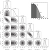 |
Fig. 4. Marginalised posterior distributions of the magnetic field strength and other parameters fitted to the NIR S I triplet. Contours correspond to 1σ, 2σ, and 3σ confidence levels. The inset in the upper right corner shows posterior distribution of the field strength with the upper limits corresponding to the same set of confidence levels indicated by different shades of grey. |
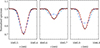 |
Fig. 5. Comparison of the S I lines in the CRIRES+ observation of o Peg (symbols) with the best-fitting non-magnetic model spectrum (solid lines). The dashed lines show an attempt at fitting the data assuming a 2 kG magnetic field. |
The final numerical results of the MCMC calculations are summarised in Table 4. For non-zero parameters, we report the median value inferred from the corresponding marginalised probability distribution along with the 1σ (13.6% and 86.4% percentiles) uncertainties. For the magnetic field strength, the 1-, 2-, and 3σ (68.3, 95.4, and 99.7% confidence levels, respectively) upper limits are given according to the marginalised probability distribution illustrated in the upper right corner of Fig. 4. The 1σ limit is 260 G, which is by far the smallest magnetic field strength limit estimated from a Stokes I spectrum of an A-type star. The non-magnetic parameters, in particular ξt and ve sin i, are well within the ranges of determinations by previous studies (e.g. Landstreet et al. 2009; Gray 2014; Adelman et al. 2015). The non-LTE S abundance derived from the NIR triplet, [S] = 0.54, is also compatible with the measurement of [S] = 0.39 ± 0.10 from the optical S I and II lines assuming LTE (Adelman et al. 2015).
Results of MCMC analysis of the S I NIR triplet.
5. Reanalysis of the Fe II 614.7–614.9 nm line pair
The Fe II 614.9 nm line is one of the most commonly used diagnostic lines for detecting Zeeman splitting in the optical spectra of early-type stars. This line has an unusual doublet Zeeman splitting pattern, with two π and two σ components coinciding in wavelength. This simple splitting pattern enables a straightforward detection of ≳ 2 kG magnetic fields in mCP stars and robust measurement of the corresponding mean field modulus ⟨B⟩ provided that the stellar projected rotational velocity does not exceed a few km s−1 (Mathys 1990, 2017; Mathys et al. 1997). Additionally, the Fe II 614.9 nm line shares the upper energy level with the nearby Fe II 614.7 nm transition, which has an almost identical oscillator strength but a very different Zeeman splitting pattern. The similarity of the formation process of these two lines prompted Mathys & Lanz (1990, 1992) to suggest using the relative intensification of this line pair – defined using the equivalent widths of these lines as δ ≡ 2(W614.7 − W614.9)/(W614.7 + W614.9) – as a proxy for the magnetic field strength for stars showing no discernible splitting of the Fe II 614.9 nm line. Based on the qualitative comparison of δ = 0.052 measured for o Peg with the relative intensification factors observed for several A stars with different magnetic field strengths, Mathys & Lanz (1990) concluded that o Peg possesses a field of ∼2 kG. This result agrees with B = 2.3 kG, which can be calculated by extrapolating the empirical linear relation between δ and B calibrated by Mathys & Lanz (1992) for the 3–5 kG ⟨B⟩ interval. The magnetic field diagnostic potential of the Fe II 614.7–614.9 nm line pair was further examined by Takeda (1991) using disc-centre polarised radiative transfer calculations, and most recently by Takeda (2023) assuming an equator-on magnetic field geometry. The former study obtained ⟨B⟩≈2–3 kG, while the latter reported ⟨B⟩ = 2.3 kG, corresponding to a polar field strength of Bd = 3.6 kG.
Despite these seemingly consistent results, detailed radiative studies of the Fe II line pair by Takeda (1991) and Kochukhov et al. (2013) uncovered several compounding factors and ambiguities in the interpretation of the equivalent-width difference of these Fe II lines in terms of the magnetic intensification. Both studies demonstrated that, in the field strength range of 0–2 kG, the relation between δ and B is neither linear nor monotonic, rendering the linear relation proposed by Mathys & Lanz (1992) unusable. Moreover, as emphasised by Kochukhov et al. (2013), the δ(B) relation depends on the assumption regarding the local magnetic field orientation, with the radial, horizontal, and turbulent magnetic fields yielding different intensification curves. At the same time, these studies did not consider the impact of the choice of atomic parameters of the Fe II lines and blending by other spectral features on the derived field strength.
Given the apparent major discrepancy between the tight upper limit of B ≤ 260 G from our NIR analysis of o Peg and repeated claims of 2–3 kG magnetic field from the optical Fe II line pair in this star, we re-examined the latter diagnostic with the spectrum synthesis methodology described in Sect. 3. The line list adopted for our modelling of the Fe II lines is provided in Table 5. It is based largely on information from VALD, with the oscillator strengths of the Fe II lines taken from Raassen & Uylings (1998). This choice yields Δlog gf = log gf614.7 − log gf614.9 = 0.014, implying that the Fe II 614.7 nm line is slightly stronger than the 614.9 nm line in the absence of magnetic field. Our line list also includes the Fe I 614.8 nm line, with the experimental log gf value from O’Brian et al. (1991). Although the importance of this blend for interpretation of the equivalent width of the Fe II 614.7 nm line has been mentioned in the literature (Mathys & Lanz 1990; Fossati et al. 2007), it appears to have been discounted in previous detailed radiative transfer studies of this Fe II line pair (Takeda 1991, 2023).
Atomic line data adopted for the analysis of the Fe II 614.7–614.9 nm line pair.
Polarised synthetic spectra were calculated in LTE with Synmast for the same atmospheric parameters as in Sect. 3, assuming a uniform radial magnetic field. Theoretical equivalent widths were obtained with direct integration of line profiles. The same approach was applied to the observed spectra published by Takeda (2023), confirming his measurement of δ = 0.0252. We estimate the uncertainty of this relative equivalent width measurement to be about 0.004, assuming S/N = 1000.
This observed δ value is compared with our theoretical δ(B) curve in Fig. 6. Taking the uncertainty of the oscillator strength of the Fe I blend into account, our calculations reproduce the observed equivalent-width difference of the two Fe II lines without the need to invoke any magnetic field. The observed δ is also compatible with our calculations at B = 2.2 kG, illustrating the ambiguity arising from a non-monotonic δ(B) relation. Figure 6 also shows another set of calculations in which the Fe I line was ignored. This shifts the intensification curve downwards, requiring B = 2.4 kG to reproduce the observed equivalent width difference. Finally, another choice of the Fe II oscillator strengths favoured by Takeda (2023)3 yields an even lower δ(B) curve, requiring a field strength of 2.7 kG to match the observed δ.
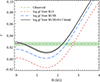 |
Fig. 6. Relative intensification of the Fe II 614.77 and 614.92 nm line pair as a function of magnetic field strength (solid line with the underlying grey curve illustrating ±1σ uncertainty arising from the oscillator strength of the Fe I 614.8 nm blend). The horizontal dash-dotted line corresponds to the observed intensification value with the ±1σ uncertainty indicated by the green rectangle. The long- and short-dashed lines show theoretical intensification curves for different choices of Fe II oscillator strength (K13: Kurucz 2013, RU98: Raassen & Uylings 1998) and blending. The two open circles indicate the line parameter-field strength combinations adopted for the synthetic calculations shown in Fig. 7. |
Thus, a measurement of the magnetic field in o Peg from equivalent widths of the Fe II line pair is generally inconclusive due to ambiguity of the δ(B) diagnostic and its dependence on the choice of line parameters. We therefore attempted to extract useful information from the line profiles themselves. Surprisingly, little attention has been paid to this approach despite high-quality observations and theoretical line-profile models being readily available. To this end, Fig. 7 compares the observed profiles published by Takeda (2023) with our Synmast calculations underlying the intensification results presented in Fig. 6. The non-magnetic theoretical spectrum was calculated with the line list from Table 5, ξt = 2 km s−1, and other stellar parameters (log NFe/Ntot, ζt, ve sin i) adjusted to fit the Fe II 614.7 nm line. It is evident that this non-magnetic calculation successfully reproduces the Fe II 614.9 nm line without the need to change any line or stellar parameters. Conversely, if we follow Takeda (2023) in adopting the oscillator strengths from Kurucz (2013), ignore the Fe I line, and use B = 2.7 kG (required to reproduce the observed δ for this choice of parameters; see Fig. 6), no consistent fit for the two lines can be obtained. In this case, the Fe II 614.9 nm line exhibits a reduced central depth and excess broadening compared to Fe II 614.7 nm, both incompatible with observations.
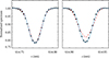 |
Fig. 7. Observed (symbols, Takeda 2023) and calculated (curves) profiles of the Fe II 614.7 and 614.9 nm lines. The solid line shows the calculation with the Fe II oscillator strengths from Raassen & Uylings (1998), blending by the Fe I 614.8 nm line, and no magnetic field. The dashed line corresponds to the synthetic spectrum computed with the oscillator strengths from Kurucz (2013), with no Fe I blending, and B = 2.7 kG. |
In summary, our reanalysis of the Fe II 614.7–614.9 nm line pair does not confirm the presence of 2–3 kG magnetic field in o Peg. Instead, the observed equivalent widths and profiles of both lines can be successfully reproduced by non-magnetic spectrum synthesis calculations with a plausible choice of transition probabilites while accounting for the contribution of the Fe I 614.8 nm blend. The traditional equivalent width-based analysis of this line pair is ambiguous, as both zero and 2–3 kG field strengths yield the same relative equivalent width difference as derived from observations. However, the strong-field solution is ruled out based on the line profile analysis.
6. Constraints on the global magnetic field
There is no evidence of circular polarisation signatures in the individual spectral lines of o Peg despite the high quality of the ESPaDOnS observations. In this case, similar to other polarimetric studies of weak magnetic fields in intermediate-mass stars (e.g. Shorlin et al. 2002; Aurière et al. 2010; Makaganiuk et al. 2011), we employed the widely used and thoroughly tested least-squares deconvolution (LSD, Donati et al. 1997; Kochukhov et al. 2010) procedure to derive very high S/N mean Stokes I and V profiles. This calculation effectively stacks profiles of all suitable metal lines under the assumption that their profiles are self-similar in velocity space and that the Stokes V signal scales with wavelength and effective Landé factor of each line according to the weak-field approximation. The line list for LSD profile calculation was obtained from the VALD database (Ryabchikova et al. 2015), using a model atmosphere with Teff = 9500 K and log g = 3.6, and elemental abundances from Adelman et al. (2015). Lines deeper than 5% of the continuum were retained and wavelength regions affected by the hydrogen Balmer lines or telluric absorption were excluded. The resulting LSD line mask contains 1483 metal lines, and is dominated by neutral and singly ionised Fe.
The LSD intensity and polarisation profiles (the latter normalised to the mean wavelength λ0 = 500 nm and effective Landé factor z0 = 1.2) derived from ESPaDOnS observations are illustrated in Fig. 8. Application of the LSD procedure resulted in a S/N gain of ∼ 40 relative to individual lines, providing a polarimetric precision of 2.4 × 10⁻⁵. Despite this, no evidence of Stokes V signatures is seen in the Stokes V LSD profiles.
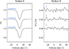 |
Fig. 8. LSD profiles of o Peg derived from archival ESPaDOnS observations. The two panels show Stokes I (left) and V (right) profiles offset vertically for display purposes. The UT observing dates are indicated above each Stokes I profile. |
The disc-averaged line-of-sight magnetic field component can be characterised by calculating the mean longitudinal magnetic field ⟨Bz⟩ from the Stokes I and V spectra (e.g. Mathys 1991; Bagnulo et al. 2002). Here we used the prescription by Wade et al. (2000) and Kochukhov et al. (2010) to derive ⟨Bz⟩ from LSD profiles. The resulting measurements are reported in the last column of Table 2. We achieve no detection of ⟨Bz⟩, with all three measurements consistent with zero field at the precision of 2.1–2.2 G.
The analysis of LSD profiles derived from high-resolution circular polarisation observations allows us to constrain global magnetic field topologies that produce null ⟨Bz⟩, such as, toroidal field or equator-on dipole. At the same time, one very specific global field configuration – a dipole closely aligned with the stellar rotational axis observed from the stellar equator – will yield no signal in Stokes V, because spectral contributions from the two stellar hemispheres will cancel out exactly for all rotational phases. This type of global magnetic field geometry, with a polar field of Bd = 2–4 kG, was advocated by Takeda (2023) to reconcile the absence of polarimetric magnetic detections in o Peg with the existence of strong field according to his analysis of intensity spectra. However, our new high-precision polarimetric measurements suggest that this magnetic configuration is highly improbable. Using the LSD profile modelling procedure described in Metcalfe et al. (2019), we established that it is sufficient for the magnetic obliquity angle β to deviate by 0.16° from 0° or 180° or for the stellar inclination angle i to deviate by the same amount from 90° for a 3 kG dipolar field to produce Stokes V signatures incompatible with observations at 3σ confidence level. Assuming random orientations of the rotational and magnetic axes, the probability that both i and β angles fall in the intervals corresponding to no detectable polarimetric signatures is < 10−8. Thus, the modern high-quality polarimetric data analysed here essentially rule out the possibility that o Peg harbours a strong large-scale magnetic field.
7. Summary and discussion
In this study, we revisited the question of the presence of a strong magnetic field at the surfaces of metallic-line stars. We focused on the bright Am star o Peg, for which the existence of 1–2 kG field covering the entire stellar surface was suggested by studies spanning three decades (Mathys & Lanz 1990; Lanz & Mathys 1993; Takeda 1991, 1993, 2023). Owing to this series of investigations, o Peg is often considered to be a prototypical Am star with a strong complex magnetic field. We re-examined archival optical spectra available for o Peg and acquired new high-resolution and high-S/N NIR spectroscopic observations using CRIRES+ at the ESO VLT. With the help of these NIR observations, we identified the S I triplet at 1046 nm as a particularly useful diagnostic for detecting Zeeman broadening signatures of magnetic field in o Peg given its large sulphur overabundance. Modelling these lines with a non-LTE polarised radiative transfer code coupled with a Bayesian inference framework, we conclude that magnetic field of o Peg cannot exceed 260 G (1σ confidence level). This represents the most sensitive magnetic field upper limit derived from the intensity spectra of an Am star.
Further re-analysis of the Fe II 614.7–614.9 nm line pair, which was previously used to claim magnetic field in o Peg, revealed the importance of the choice of atomic line parameters and accounting for weak blending. We show that the observed relative intensification of these lines can be reproduced with either non-magnetic calculations or > 2 kG magnetic field, depending on the adopted line list. However, the profile shape, in particular that of the 614.9 nm Fe II line, is incompatible with the strong-field solution. In summary, both the optical and NIR spectroscopic data suggest that o Peg does not possess a kG-strength magnetic field. If any surface field is present in this star, its strength does not exceed a few hundred G.
The outcome of our reassessment of the magnetic interpretation of the relative intensification of the Fe II 614.7–614.9 nm lines in o Peg is reminiscent of the results of investigations of these lines in the spectra of HgMn stars. For these objects, often considered hotter analogues of Am stars, complex kG-strength magnetic fields claimed from the Fe II line strengths (Hubrig et al. 1999; Hubrig & Castelli 2001) were shown to be incompatible with the lack of Zeeman broadening in high-resolution spectra (Kochukhov et al. 2013). The line intensification analysis was also similarly jeopardised by blending in some HgMn targets (Takada-Hidai & Jugaku 1992). This experience for two distinct classes of CP stars suggests that using the relative intensification of this Fe II line pair to infer magnetic field strength tends to yield spurious results when extrapolated outside the empirically calibrated 3–5 kG field strength interval (Mathys & Lanz 1992). Therefore, some of the recent magnetic field strength estimates employing the Fe II line ratio (e.g. Holdsworth et al. 2014, 2016; Smalley et al. 2015; Murphy et al. 2020) may not be trustworthy, even when applied to the types of CP stars expected to host strong magnetic fields.
In addition to the analysis of Zeeman broadening and magnetic intensification in Stokes I spectra, we obtained complementary information on the global magnetic field of o Peg using unpublished archival optical circular polarisation spectra collected with ESPaDOnS at CFHT. Three observations spread over 10 nights yield null mean longitudinal magnetic field measurements with a typical uncertainty of 2 G. This represents a ten-fold precision improvement compared to the previous ⟨Bz⟩ determinations for o Peg (Shorlin et al. 2002; Bychkov et al. 2009). Moreover, we report no evidence of polarisation signatures in S/N ≈ 40 000 LSD Stokes V profiles, ruling out the presence of moderately complex non-dipolar global magnetic field topologies.
The non-detection of a magnetic field in polarimetric observables does not necessarily rule out that the star hosts a sizeable surface magnetic field. It can be argued, as was done in previous studies of o Peg, that the star possesses a dipolar field that happened to be observed nearly equator-on (Takeda 2023) or that the stellar surface field lacks any global component (Mathys & Lanz 1990). However, the high polarimetric accuracy of the Stokes V LSD profiles derived in our study challenges both of these hypotheses. To remain consistent with the polarimetric non-detections in all three Stokes V observations, the stellar and dipolar field axes must have a very particular orientation. Namely, both the inclination and magnetic obliquity angles must not deviate by more than ≈0.2° from 90° and 0° or 180°, respectively. We show that the probability of encountering such a magnetic configuration is negligible. On the other hand, the second hypothesis of a highly tangled magnetic field implies a ratio of the total to global field strength of ∼103 if one adopts the ∼2 kG total field strength advocated by previous studies of o Peg. Although situations where ⟨Bz⟩≪⟨B⟩ are not unheard of in stellar magnetometry, this ratio appears to be extremely large for o Peg compared to 101–102 total to global field amplitudes found in cool active stars with dynamo fields (Kochukhov et al. 2020; Kochukhov 2021). Thus, to accommodate the low ⟨Bz⟩ and high ⟨B⟩ for o Peg, a qualitatively new type of magnetic field generation process would be required that can produce a highly structured surface field with a degree of complexity not seen in any other types of stars. However, our results point to a more prosaic explanation: the previous claims of 1–2 kG complex field in o Peg are erroneous and the actual total field strength does not exceed a few hundred G according to the most sensitive NIR diagnostic. Therefore, this star should be considered non-magnetic according to the most sensitive polarimetric and spectroscopic magnetic field detection analyses.
Taking into account the results of the present study as well as recent literature, there is no evidence that either globally organised or complex kG-strength magnetic fields exist on the surfaces of Am stars. Instead, Am stars observed with sufficient polarimetric precision appear to possess ultraweak sub-G fields (Petit et al. 2011; Blazère et al. 2016; Neiner et al. 2017) of unknown geometry. Thus, our work reaffirms the presence of a ‘magnetic desert’ – a conspicuous two orders of magnitude gap in the field strength distribution between the 100–300 G lower field strength bound of mCP stars (Aurière et al. 2007; Kochukhov et al. 2023a) and the sub-G fields of Am stars. The only CP star known to straddle this gap is the marginal Am star γ Gem, which hosts a dipolar field with a polar strength of ≈30 G (Blazère et al. 2020). It remains to be seen whether this object is part of a larger population or represents an extreme example of an mCP star that is in the process of losing its fossil magnetic field.
This value is significantly smaller than δ = 0.052 reported for o Peg by Mathys & Lanz (1990). We have no explanation for this discrepancy, nor for why this reduction of the observed δ did not result in a corresponding decrease in the field strength inferred by Takeda (2023) compared to Takeda (1991).
We used log gf614.7 = −2.731 and log gf614.9 = −2.732 according to the semi-empirical calculations by Kurucz (2013). Takeda (2023) adopted log gf614.7 = −2.721 and log gf614.9 = −2.724 corresponding to an older version of Kurucz’s calculations. In both cases, the resulting Δlog gf is smaller than for the oscillator strengths from Raassen & Uylings (1998).
Acknowledgments
O.K. acknowledges support by the Swedish Research Council (grant agreements no. 2019-03548 and 2023-03667), the Swedish National Space Agency, and the Royal Swedish Academy of Sciences. A.M.A. acknowledges support from the Swedish Research Council (grant agreement no. 2020-03940). H.L.R. acknowledges the support of the DFG priority program SPP 1992 “Exploring the Diversity of Extrasolar Planets (RE 1664/20-1)”. E.N. acknowledges the support by the DFG Research Unit FOR2544 “Blue Planets around Red Stars”. K.P. acknowledges the Swiss National Science Foundation, grant number 217195, for financial support. M.R. acknowledges the support by the DFG priority program SPP 1992 “Exploring the Diversity of Extrasolar Planets” (DFG PR 36 24602/41). D.S. acknowledges financial support from the project PID2021-126365NB-C21 funded by Agencia Estatal de Investigación of the Ministerio de Ciencia e Innovación (MCIN/AEI/10.12039/501100011033). CRIRES+ is an ESO upgrade project carried out by Thüringer Landessternwarte Tautenburg, Georg-August Universität Göttingen, and Uppsala University. The project is funded by the Federal Ministry of Education and Research (Germany) through Grants 05A11MG3, 05A14MG4, 05A17MG2 and the Wallenberg Foundation.
References
- Adelman, S. J. 1988, MNRAS, 230, 671 [NASA ADS] [CrossRef] [Google Scholar]
- Adelman, S. J., Cowley, C. R., Leckrone, D. S., Roby, S. W., & Wahlgren, G. M. 1993, ApJ, 419, 276 [CrossRef] [Google Scholar]
- Adelman, S. J., Gulliver, A. F., & Heaton, R. J. 2015, PASP, 127, 58 [NASA ADS] [CrossRef] [Google Scholar]
- Albrow, M. D., & Cottrell, P. L. 1996, MNRAS, 278, 337 [NASA ADS] [Google Scholar]
- Allen, C. W. 1973, Astrophysical Quantities (London: Athlone Press) [Google Scholar]
- Amarsi, A. M. 2015, MNRAS, 452, 1612 [NASA ADS] [CrossRef] [Google Scholar]
- Amarsi, A. M., Barklem, P. S., Asplund, M., Collet, R., & Zatsarinny, O. 2018a, A&A, 616, A89 [NASA ADS] [CrossRef] [EDP Sciences] [Google Scholar]
- Amarsi, A. M., Nordlander, T., Barklem, P. S., et al. 2018b, A&A, 615, A139 [NASA ADS] [CrossRef] [EDP Sciences] [Google Scholar]
- Amarsi, A. M., Liljegren, S., & Nissen, P. E. 2022, A&A, 668, A68 [NASA ADS] [CrossRef] [EDP Sciences] [Google Scholar]
- Anfinogentov, S. A., Nakariakov, V. M., Pascoe, D. J., & Goddard, C. R. 2021, ApJS, 252, 11 [Google Scholar]
- Anstee, S. D., & O’Mara, B. J. 1995, MNRAS, 276, 859 [Google Scholar]
- Aurière, M., Wade, G. A., Silvester, J., et al. 2007, A&A, 475, 1053 [NASA ADS] [CrossRef] [EDP Sciences] [Google Scholar]
- Aurière, M., Wade, G. A., Lignières, F., et al. 2010, A&A, 523, A40 [NASA ADS] [CrossRef] [EDP Sciences] [Google Scholar]
- Bagnulo, S., Szeifert, T., Wade, G. A., Landstreet, J. D., & Mathys, G. 2002, A&A, 389, 191 [NASA ADS] [CrossRef] [EDP Sciences] [Google Scholar]
- Barklem, P. S. 2016, A&A Rev., 24, 9 [NASA ADS] [CrossRef] [Google Scholar]
- Barklem, P. S., & O’Mara, B. J. 1997, MNRAS, 290, 102 [Google Scholar]
- Barklem, P. S., O’Mara, B. J., & Ross, J. E. 1998, MNRAS, 296, 1057 [Google Scholar]
- Barklem, P. S., Piskunov, N., & O’Mara, B. J. 2000, A&AS, 142, 467 [NASA ADS] [CrossRef] [EDP Sciences] [Google Scholar]
- Belyaev, A. K., & Voronov, Y. V. 2020, ApJ, 893, 59 [NASA ADS] [CrossRef] [Google Scholar]
- Blazère, A., Petit, P., Lignières, F., et al. 2016, A&A, 586, A97 [NASA ADS] [CrossRef] [EDP Sciences] [Google Scholar]
- Blazère, A., Petit, P., Neiner, C., et al. 2020, MNRAS, 492, 5794 [CrossRef] [Google Scholar]
- Bychkov, V. D., Bychkova, L. V., & Madej, J. 2009, MNRAS, 394, 1338 [NASA ADS] [CrossRef] [Google Scholar]
- Caffau, E., Andrievsky, S., Korotin, S., et al. 2016, A&A, 585, A16 [NASA ADS] [CrossRef] [EDP Sciences] [Google Scholar]
- Cantiello, M., & Braithwaite, J. 2019, ApJ, 883, 106 [Google Scholar]
- Carlos, M., Amarsi, A. M., & Nissen, P. E. 2024, ApJ, submitted [Google Scholar]
- Carrier, F., North, P., Udry, S., & Babel, J. 2002, A&A, 394, 151 [NASA ADS] [CrossRef] [EDP Sciences] [Google Scholar]
- Cowley, C. R., Ayres, T. R., Castelli, F., et al. 2016, ApJ, 826, 158 [CrossRef] [Google Scholar]
- Debernardi, Y., Mermilliod, J. C., Carquillat, J. M., & Ginestet, N. 2000, A&A, 354, 881 [NASA ADS] [Google Scholar]
- Donati, J.-F., & Landstreet, J. D. 2009, ARA&A, 47, 333 [NASA ADS] [CrossRef] [Google Scholar]
- Donati, J. F., Semel, M., Carter, B. D., Rees, D. E., & Collier Cameron, A. 1997, MNRAS, 291, 658 [Google Scholar]
- Donati, J., Catala, C., Landstreet, J. D., & Petit, P. 2006, ASP Conf. Ser., 358, 362 [NASA ADS] [Google Scholar]
- Dorn, R. J., Bristow, P., Smoker, J. V., et al. 2023, A&A, 671, A24 [NASA ADS] [CrossRef] [EDP Sciences] [Google Scholar]
- Drake, S. A., Linsky, J. L., & Bookbinder, J. A. 1994, AJ, 108, 2203 [NASA ADS] [CrossRef] [Google Scholar]
- Dworetsky, M. M. 1993, ASP Conf. Ser., 44, 1 [NASA ADS] [Google Scholar]
- Fossati, L., Bagnulo, S., Monier, R., et al. 2007, A&A, 476, 911 [NASA ADS] [CrossRef] [EDP Sciences] [Google Scholar]
- Ghazaryan, S., Alecian, G., & Hakobyan, A. A. 2018, MNRAS, 480, 2953 [NASA ADS] [CrossRef] [Google Scholar]
- Gray, D. F. 2014, AJ, 147, 81 [NASA ADS] [CrossRef] [Google Scholar]
- Grunhut, J. H., Wade, G. A., Neiner, C., et al. 2017, MNRAS, 465, 2432 [NASA ADS] [CrossRef] [Google Scholar]
- Hahlin, A., Kochukhov, O., Rains, A. D., et al. 2023, A&A, 675, A91 [NASA ADS] [CrossRef] [EDP Sciences] [Google Scholar]
- Holdsworth, D. L., Smalley, B., Kurtz, D. W., et al. 2014, MNRAS, 443, 2049 [CrossRef] [Google Scholar]
- Holdsworth, D. L., Kurtz, D. W., Smalley, B., et al. 2016, MNRAS, 462, 876 [NASA ADS] [CrossRef] [Google Scholar]
- Hubrig, S., & Castelli, F. 2001, A&A, 375, 963 [NASA ADS] [CrossRef] [EDP Sciences] [Google Scholar]
- Hubrig, S., & Schöller, M. 2021, Magnetic Fields in O, B, and A Stars (Bristol: IOP Publishing) [Google Scholar]
- Hubrig, S., Castelli, F., & Wahlgren, G. M. 1999, A&A, 346, 139 [NASA ADS] [Google Scholar]
- Hui-Bon-Hoa, A. 2000, A&AS, 144, 203 [NASA ADS] [CrossRef] [EDP Sciences] [Google Scholar]
- Jermyn, A. S., & Cantiello, M. 2020, ApJ, 900, 113 [NASA ADS] [CrossRef] [Google Scholar]
- Kamp, I., Iliev, I. K., Paunzen, E., et al. 2001, A&A, 375, 899 [NASA ADS] [CrossRef] [EDP Sciences] [Google Scholar]
- Kaulakys, B. 1991, J. Phys. B A. Mol. Phys., 24, L127 [CrossRef] [Google Scholar]
- Kochukhov, O. 2007, in Physics of Magnetic Stars, eds. I. I. Romanyuk, & D. O. Kudryavtsev, 109 [Google Scholar]
- Kochukhov, O. 2021, A&A Rev., 29, 1 [NASA ADS] [CrossRef] [Google Scholar]
- Kochukhov, O., & Lavail, A. 2017, ApJ, 835, L4 [Google Scholar]
- Kochukhov, O., Makaganiuk, V., & Piskunov, N. 2010, A&A, 524, A5 [NASA ADS] [CrossRef] [EDP Sciences] [Google Scholar]
- Kochukhov, O., Makaganiuk, V., Piskunov, N., et al. 2013, A&A, 554, A61 [NASA ADS] [CrossRef] [EDP Sciences] [Google Scholar]
- Kochukhov, O., Hackman, T., Lehtinen, J. J., & Wehrhahn, A. 2020, A&A, 635, A142 [NASA ADS] [CrossRef] [EDP Sciences] [Google Scholar]
- Kochukhov, O., Gürsoytrak Mutlay, H., Amarsi, A. M., et al. 2023a, MNRAS, 521, 3480 [NASA ADS] [CrossRef] [Google Scholar]
- Kochukhov, O., Hackman, T., & Lehtinen, J. J. 2023b, A&A, 680, L17 [NASA ADS] [CrossRef] [EDP Sciences] [Google Scholar]
- Korčáková, D., Sestito, F., Manset, N., et al. 2022, A&A, 659, A35 [NASA ADS] [CrossRef] [EDP Sciences] [Google Scholar]
- Korotin, S. A. 2009, Astron. Rep., 53, 651 [Google Scholar]
- Kramida, A., Ralchenko, Y., Reader, J., & NIST ASD Team 2022, NIST Atomic Spectra Database, ver. 5.10 [Online], https://physics.nist.gov/asd, National Institute of Standards and Technology Gaithersburg, MD [Google Scholar]
- Kurtz, D. W., & Martinez, P. 2000, Bal. Astron., 9, 253 [Google Scholar]
- Kurucz, R. L. 1995, ASP Conf. Ser., 78, 205 [NASA ADS] [Google Scholar]
- Kurucz, R. L. 2013, Robert L. Kurucz On-line Database of Observed and Predicted Atomic Transitions [Google Scholar]
- Landi Degl’Innocenti, E., & Landolfi, M. 2004, Polarization in Spectral Lines (Kluwer Academic Publishers), Astrophys. Space Sci. Lib., 307 [Google Scholar]
- Landstreet, J. D. 1992, A&A Rev., 4, 35 [NASA ADS] [CrossRef] [Google Scholar]
- Landstreet, J. D. 2011, A&A, 528, A132 [NASA ADS] [CrossRef] [EDP Sciences] [Google Scholar]
- Landstreet, J. D., Kupka, F., Ford, H. A., et al. 2009, A&A, 503, 973 [NASA ADS] [CrossRef] [EDP Sciences] [Google Scholar]
- Langhoff, P. W., Sims, J., & Corcoran, C. T. 1974, Phys. Rev. A, 10, 829 [CrossRef] [Google Scholar]
- Lanz, T., & Mathys, G. 1993, A&A, 280, 486 [NASA ADS] [Google Scholar]
- Lavail, A., Kochukhov, O., & Hussain, G. A. J. 2019, A&A, 630, A99 [NASA ADS] [CrossRef] [EDP Sciences] [Google Scholar]
- Lee, H.-W., & Kim, H. I. 2004, MNRAS, 347, 802 [NASA ADS] [CrossRef] [Google Scholar]
- Leenaarts, J., & Carlsson, M. 2009, ASP Conf. Ser., 415, 87 [Google Scholar]
- Lind, K., & Amarsi, A. M. 2024, ARA&A, accepted [arXiv:2401.00697] [Google Scholar]
- Makaganiuk, V., Kochukhov, O., Piskunov, N., et al. 2011, A&A, 525, A97 [CrossRef] [EDP Sciences] [Google Scholar]
- Mathys, G. 1990, A&A, 232, 151 [NASA ADS] [Google Scholar]
- Mathys, G. 1991, A&AS, 89, 121 [NASA ADS] [Google Scholar]
- Mathys, G. 2004a, in The A-Star Puzzle, eds. J. Zverko, J. Ziznovsky, S. J. Adelman, & W. W. Weiss, IAU Symp., 224, 225 [NASA ADS] [Google Scholar]
- Mathys, G. 2004b, in Stellar Rotation, eds. A. Maeder, & P. Eenens, IAU Symp., 215, 270 [NASA ADS] [Google Scholar]
- Mathys, G. 2009, ASP Conf. Ser., 405, 473 [NASA ADS] [Google Scholar]
- Mathys, G. 2017, A&A, 601, A14 [NASA ADS] [CrossRef] [EDP Sciences] [Google Scholar]
- Mathys, G., & Lanz, T. 1990, A&A, 230, L21 [NASA ADS] [Google Scholar]
- Mathys, G., & Lanz, T. 1992, A&A, 256, 169 [NASA ADS] [Google Scholar]
- Mathys, G., Hubrig, S., Landstreet, J. D., Lanz, T., & Manfroid, J. 1997, A&AS, 123, 353 [NASA ADS] [CrossRef] [EDP Sciences] [Google Scholar]
- Metcalfe, T. S., Kochukhov, O., Ilyin, I. V., et al. 2019, ApJ, 887, L38 [NASA ADS] [CrossRef] [Google Scholar]
- Murphy, S. J., Saio, H., Takada-Hidai, M., et al. 2020, MNRAS, 498, 4272 [NASA ADS] [CrossRef] [Google Scholar]
- Neiner, C., Wade, G. A., & Sikora, J. 2017, MNRAS, 468, L46 [NASA ADS] [CrossRef] [Google Scholar]
- Nissen, P. E., Akerman, C., Asplund, M., et al. 2007, A&A, 469, 319 [NASA ADS] [CrossRef] [EDP Sciences] [Google Scholar]
- O’Brian, T. R., Wickliffe, M. E., Lawler, J. E., Whaling, W., & Brault, J. W. 1991, J. Opt. Soc. Am. B Opt. Phys., 8, 1185 [Google Scholar]
- Petit, P., Lignières, F., Aurière, M., et al. 2011, A&A, 532, L13 [NASA ADS] [CrossRef] [EDP Sciences] [Google Scholar]
- Petit, P., Louge, T., Théado, S., et al. 2014, PASP, 126, 469 [NASA ADS] [CrossRef] [Google Scholar]
- Piskunov, N., & Valenti, J. A. 2017, A&A, 597, A16 [NASA ADS] [CrossRef] [EDP Sciences] [Google Scholar]
- Preston, G. W. 1974, ARA&A, 12, 257 [Google Scholar]
- Raassen, A. J. J., & Uylings, P. H. M. 1998, A&A, 340, 300 [Google Scholar]
- Rosén, L., Kochukhov, O., Alecian, E., et al. 2018, A&A, 613, A60 [Google Scholar]
- Rutten, R. J. 2003, Radiative Transfer in Stellar Atmospheres (Utrecht University lecture notes) [Google Scholar]
- Ryabchikova, T., Piskunov, N., Kurucz, R. L., et al. 2015, Phys. Scr., 90, 054005 [Google Scholar]
- Savanov, I. S. 1994, Astrophysics, 37, 112 [NASA ADS] [CrossRef] [Google Scholar]
- Schöller, M., Hubrig, S., Fossati, L., et al. 2017, A&A, 599, A66 [NASA ADS] [CrossRef] [EDP Sciences] [Google Scholar]
- Scholz, G., Lehmann, H., Harmanec, P., Gerth, E., & Hildebrandt, G. 1997, A&A, 320, 791 [Google Scholar]
- Scott, P., Grevesse, N., Asplund, M., et al. 2015, A&A, 573, A25 [NASA ADS] [CrossRef] [EDP Sciences] [Google Scholar]
- Seaton, M. J., Zeippen, C. J., Tully, J. A., et al. 1992, Rev. Mex. Astron. Astrofis., 23, 19 [NASA ADS] [EDP Sciences] [Google Scholar]
- Shorlin, S. L. S., Wade, G. A., Donati, J.-F., et al. 2002, A&A, 392, 637 [NASA ADS] [CrossRef] [EDP Sciences] [Google Scholar]
- Shulyak, D., Tsymbal, V., Ryabchikova, T., Stütz, C., & Weiss, W. W. 2004, A&A, 428, 993 [NASA ADS] [CrossRef] [EDP Sciences] [Google Scholar]
- Sikora, J., Wade, G. A., Power, J., & Neiner, C. 2019, MNRAS, 483, 2300 [NASA ADS] [CrossRef] [Google Scholar]
- Smalley, B., Niemczura, E., Murphy, S. J., et al. 2015, MNRAS, 452, 3334 [NASA ADS] [CrossRef] [Google Scholar]
- Smith, K. C. 1996, Ap&SS, 237, 77 [NASA ADS] [CrossRef] [Google Scholar]
- Takada-Hidai, M., & Jugaku, J. 1992, PASP, 104, 106 [NASA ADS] [CrossRef] [Google Scholar]
- Takada-Hidai, M., & Jugaku, J. 1993, ASP Conf. Ser., 44, 310 [NASA ADS] [Google Scholar]
- Takeda, Y. 1991, PASJ, 43, 823 [NASA ADS] [Google Scholar]
- Takeda, Y. 1993, PASJ, 45, 453 [NASA ADS] [Google Scholar]
- Takeda, Y. 2023, Astron. Nachr., 344 [CrossRef] [Google Scholar]
- Takeda, Y., Hashimoto, O., Taguchi, H., et al. 2005, PASJ, 57, 751 [NASA ADS] [Google Scholar]
- Takeda, Y., Kang, D.-I., Han, I., et al. 2012, PASJ, 64, 38 [NASA ADS] [CrossRef] [Google Scholar]
- van Regemorter, H. 1962, ApJ, 136, 906 [NASA ADS] [CrossRef] [Google Scholar]
- Wade, G. A., Donati, J.-F., Landstreet, J. D., & Shorlin, S. L. S. 2000, MNRAS, 313, 851 [CrossRef] [Google Scholar]
- Wade, G. A., Bagnulo, S., Kochukhov, O., et al. 2001, A&A, 374, 265 [NASA ADS] [CrossRef] [EDP Sciences] [Google Scholar]
- Zatsarinny, O., & Bartschat, K. 2006, J. Phys. B Atomic Mol. Phys., 39, 2861 [CrossRef] [Google Scholar]
- Zerne, R., Caiyan, L., Berzinsh, U., & Svanberg, S. 1997, Phys. Scr., 56, 459 [NASA ADS] [CrossRef] [Google Scholar]
- Zhou, Y., Amarsi, A. M., Aguirre Børsen-Koch, V., et al. 2023, A&A, 677, A98 [NASA ADS] [CrossRef] [EDP Sciences] [Google Scholar]
All Tables
Mean longitudinal magnetic field measurements derived from the ESPaDOnS observations.
Atomic line data adopted for the analysis of the Fe II 614.7–614.9 nm line pair.
All Figures
|
Fig. 1. Behaviour of the NIR S I triplet in magnetic field. (a) Synthetic Zeeman profiles for different magnetic field strengths. The corresponding splitting patterns are shown schematically above each line for B = 3 kG. (b) Comparison of the Zeeman (black dashed line) and PPB (red solid line) calculations for B = 3 kG. The splitting patterns above the line profiles are illustrated for the PPB case. |
| In the text | |
|
Fig. 2. Impact of departures from LTE on the synthetic profiles of the NIR S I triplet. These calculations were carried out for B = 0 kG, log NS/Ntot = −4.35, ξt = 2 km s−1, and other parameters of o Peg set to the best-fitting values found in Sect. 4. |
| In the text | |
|
Fig. 3. Departure coefficients of the lower and upper levels of the S I triplet, bl and bu, respectively. Their ratio is also shown. The full-width at half maximum (arrows) and peak depth (open circles) of the contribution functions to the depression in the disc-integrated flux – calculated at line centre – are shown for the three lines of the S I triplet. |
| In the text | |
|
Fig. 4. Marginalised posterior distributions of the magnetic field strength and other parameters fitted to the NIR S I triplet. Contours correspond to 1σ, 2σ, and 3σ confidence levels. The inset in the upper right corner shows posterior distribution of the field strength with the upper limits corresponding to the same set of confidence levels indicated by different shades of grey. |
| In the text | |
|
Fig. 5. Comparison of the S I lines in the CRIRES+ observation of o Peg (symbols) with the best-fitting non-magnetic model spectrum (solid lines). The dashed lines show an attempt at fitting the data assuming a 2 kG magnetic field. |
| In the text | |
|
Fig. 6. Relative intensification of the Fe II 614.77 and 614.92 nm line pair as a function of magnetic field strength (solid line with the underlying grey curve illustrating ±1σ uncertainty arising from the oscillator strength of the Fe I 614.8 nm blend). The horizontal dash-dotted line corresponds to the observed intensification value with the ±1σ uncertainty indicated by the green rectangle. The long- and short-dashed lines show theoretical intensification curves for different choices of Fe II oscillator strength (K13: Kurucz 2013, RU98: Raassen & Uylings 1998) and blending. The two open circles indicate the line parameter-field strength combinations adopted for the synthetic calculations shown in Fig. 7. |
| In the text | |
|
Fig. 7. Observed (symbols, Takeda 2023) and calculated (curves) profiles of the Fe II 614.7 and 614.9 nm lines. The solid line shows the calculation with the Fe II oscillator strengths from Raassen & Uylings (1998), blending by the Fe I 614.8 nm line, and no magnetic field. The dashed line corresponds to the synthetic spectrum computed with the oscillator strengths from Kurucz (2013), with no Fe I blending, and B = 2.7 kG. |
| In the text | |
|
Fig. 8. LSD profiles of o Peg derived from archival ESPaDOnS observations. The two panels show Stokes I (left) and V (right) profiles offset vertically for display purposes. The UT observing dates are indicated above each Stokes I profile. |
| In the text | |
Current usage metrics show cumulative count of Article Views (full-text article views including HTML views, PDF and ePub downloads, according to the available data) and Abstracts Views on Vision4Press platform.
Data correspond to usage on the plateform after 2015. The current usage metrics is available 48-96 hours after online publication and is updated daily on week days.
Initial download of the metrics may take a while.