| Issue |
A&A
Volume 689, September 2024
|
|
|---|---|---|
| Article Number | A288 | |
| Number of page(s) | 10 | |
| Section | Stellar structure and evolution | |
| DOI | https://doi.org/10.1051/0004-6361/202450523 | |
| Published online | 20 September 2024 | |
Searching for the stellar cycles of low-mass stars using TESS data
1
Armagh Observatory and Planetarium, College Hill, Armagh, BT61 9DG, N. Ireland, UK
2
Finnish Centre for Astronomy with ESO (FINCA), Quantum, Vesilinnantie 5, FI-20014 University of Turku, Finland
Received:
26
April
2024
Accepted:
9
July
2024
We carried out a search for stellar activity cycles in late low-mass M dwarfs (M0–M6) located in the TESS northern and southern continuous viewing zones using data from sectors 1–61 (Cycle 1 to partway through Cycle 5). We utilised TESS-SPOC data, which initially had a cadence of 30 min and was then reduced to 10 min in Cycle 3. In addition, we required for each star to be observed in at least six sectors in each north and south Cycle: 1950 low-mass stars ultimately met these criteria. Strong evidence was seen in 245 stars for a very stable photometric variation that we assumed to be a signature of the stars’ rotation period. We conducted a similar study for solar-like stars and found that 194 out of 1432 stars had a very stable modulation. We then searched for evidence of a variation in the rotational amplitude. We found 26 low-mass stars that showed evidence of variability in their photometric amplitude and only one solar-like star. Some display a monotonic trend over 3–4 years, whilst others reveal shorter term variations. We determined the predicted cycle durations of these stars using a relationship found in the literature and an estimate of the stars’ Rossby number. Finally, we found a marginally statistically significant correlation between the range in the rotational amplitude modulation and the rotation period.
Key words: stars: activity / stars: flare / stars: late-type / stars: low-mass / stars: rotation
© The Authors 2024
 Open Access article, published by EDP Sciences, under the terms of the Creative Commons Attribution License (https://creativecommons.org/licenses/by/4.0), which permits unrestricted use, distribution, and reproduction in any medium, provided the original work is properly cited.
This article is published in open access under the Subscribe to Open model. Subscribe to A&A to support open access publication.
1. Introduction
Low-mass stars account for nearly three-quarters of the stars in our local neighbourhood (Henry et al. 2006). In spite of this, over the last few decades, a more intense focus has been renewed for these low-luminosity stars. Within the MV spectral type, stars exhibit masses in the range of 0.08–0.6 M⊙ (M9V–M0V), becoming fully convective around the early-to-mid M type. The reason for the renewed interest in these stars is due to exoplanets producing a greater transit depth in these small stars, thereby making them easier to detect. Furthermore, many of these stars are active, especially fully convective stars (e.g. Pettersen 1989), which provides an insight into how fully convective stars generate and sustain a global magnetic field. This topic is of interest to the field of magnetism in general.
Moreover, the instruments to study stars of all kinds has radically changed since the first exoplanets were detected. Prior to the launch of CoRot and Kepler, several groups attempted ground-based multi-telescope observations of single stars (e.g. Rodono et al. 1986; Doyle et al. 1988a, 1988b, 1993). What these series of space missions facilitated (amongst many other things) was the measurement of the rotation period for a large number of stars (McQuillan et al. 2014) and a comprehensive search for flares from stars with a wide range of spectral type (Davenport 2016). In turn, this allows for the determination of how the stellar rotation period varies as a function of age and mass (Rebull et al. 2016) as well as how the rate of flares from an active host star can affect the atmosphere of any orbiting exoplanet (Konings et al. 2022).
Determining the rotation period of low-mass stars is usually based on the assumption that any modulation in the star’s light curve is due to the rotation of a starspot(s) that come in and out of view as the star rotates. For stars whose rotation axis is viewed near face-on, it is expected that the starspot(s) would remain in view and show no modulation unless the spot coverage varied over time. Initially, it was assumed that a single large spot group caused the modulation in a star’s flux, with any variations in the rotation flux profile due to changes in the spot distribution or that additional starspots emerged. However, it has been shown that single filter photometry data can be reproduced by a wide range of spot distribution, sizes, inclinations, and spot temperatures (Jackson & Jeffries 2013; Luger et al. 2021a). On the other hand, Luger et al. (2021b) argued that some degeneracies in the spot distributions can be broken by analysing the light curve of many stars with broadly similar properties.
Although there is still some uncertainty in terms of mapping the distribution of spots over the surface of these stars, progress has been made in searching for activity cycles on stars other than the Sun. The solar cycle lasts ∼11 yr (strictly speaking ∼22 yr) and manifests itself through the changing number of sunspots; emission in the core of the Ca II H&K lines; X-ray flux; and the number of flares and coronal mass ejections (CMEs). Given the timescales expected (years), finding evidence for stellar activity cycles have taken time to emerge. Systematic and regular spectroscopic observations of solar-like stars began during the 1960s with a focus on using the Ca II H&K lines as an activity indicator (Wilson 1968). Subsequent studies using data such as these showed that other stars exhibit activity cycles on a similar timescale to the Sun (e.g. Baliunas et al. 1995 and references therein). For lower mass stars, an activity cycle of ∼7 yr was detected in the star nearest to the Sun, Proxima Centauri (M5.5Ve), using optical, UV, and X-ray observations (Wargelin et al. 2017). Furthermore, Ibañez Bustos et al. (2020) used Ca II H&K lines to determine a stellar cycle of ∼4 yr in the M4V Gl 729. Küker et al. (2019) reviewed observations that appear to show that fast-rotating M dwarfs have cycles of a year but increase to around four years for slower rotators. However, fast rotators cannot be understood by an advection-dominated dynamo model.
In principle, ground-based optical photometric observations that are stable and free from systematic trends can be used to detect activity cycles as long as the timeline is sufficiently long. Since 2018, the TESS satellite has gradually been building up a set of observations of stars covering most of the sky. This is particulary true for stars within ∼11° of the north and south ecliptic poles (the ‘continuous viewing zones’) since they can be observed for nearly one year with a return visit one year later. However, since these light curves are not flux-calibrated, low-amplitude, long-term modulations or trends can be difficult to detect in a robust manner.
An alternative means is to search for variations in the amplitude of the rotational modulation over time (Berdyugina & Järvinen 2005). Using this approach, Suárez Mascareño et al. (2016) determined that two K type stars showed periods of 10.2 and 8.7 yr. Reinhold et al. (2017) used Kepler data to study the light curves of 23601 stars and used the generalised Lomb-Scargle periodgram (LSP) to search for variations in the rotational amplitude over time. They found amplitude periodicities in 3203 stars, with some weak evidence that the cycle period increased for longer rotation periods. Most of the stars in that sample had spectral types earlier than MV stars. For a recent review of activity cycles on stars other than Sun, we refer to Jeffers et al. (2023).
In this exploratory study we, use TESS data of low-mass stars located in the north and south continuous viewing zones on two occasions to assess how stable the dominant period in their light curves is. For stars that showed very stable periods, we searched for amplitude variations that may reveal evidence of stellar activity cycles.
2. TESS sample
The TESS satellite was launched into an Earth orbit with a period of 13.7 d. It has four 10.5 cm telescopes that observe a 24° × 90° instantaneous strip of sky (a sector) for ∼27 d (see Ricker et al. 2015, for details). In the first year (Cycle 1), TESS covered most of the southern ecliptic hemisphere and in the second year (Cycle 2), it covered the northern ecliptic hemisphere, although with less sky coverage than Cycle 1 to avoid contamination from stray light from the Earth and Moon. In both cycles, there is an area around the ecliptic poles which are visible in each sector. In Cycle 3, the field pointings mirrored Cycle 1 and in Cycle 4, some sectors observed in Cycle 2 were observed again in addition to some fields not previous observed. In Cycles 1 and 2, full frame images were obtained every 30 min, which increased to every 10 min in Cycles 3 and 4. From the start, the Guest Observer programme was able to populate targets which were observed in a 2-min cadence, with a 20 s cadence option becoming available in Cycles 3 and 4.
We used the Gaia EDR3 catalogue of stars within 100 pc (Smart et al. 2021) and using their (BP − RP) colours and MG absolute magnitudes, we were able to select the ones with an equivalent spectral type later than ∼M0V and were on, or close to, the main sequence. We then cross matched this sample with those stars which had TESS light curves derived using the TESS Science Processing Operations Center FFI Target List Products (SPOC, Caldwell 2020) that uses the full-frame images to extract light curves (we searched light curves from TESS sectors 0–61). Since our aim was to search for variations in the amplitude of the main period, we then restricted our sample to require a star to have been observed in at least six sectors. Finally, since the pixel size of TESS (21″ per pixel) is sufficiently large to include spatially nearby bright stars to contaminate the resulting light curve, we filtered stars so the contamination ratio (Stassun et al. 2018) (i.e. the fraction of the flux from other spatially nearby stars) is < 0.1. We show in Figure 1 the 1950 stars which are our M dwarf sample. For a comparison, we also obtained a solar-like sample using the same criteria as for M dwarfs, where we took stars close to the main sequence for 0.6 < (BP − RP) < 1.1 (F5V–K2V, Pecaut & Mamajek (2013)): we identified 1432 stars, which are shown as green dots in Figure 1.
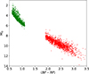 |
Fig. 1. Gaia HRD (BP − RP, MG) of low-mass stars (red) and solar type stars (green) that were observed for at least six sectors in each TESS Cycle. |
3. Data analysis
Each sector of data was normalised so its mean was unity and then clipped to remove data that were 5σ deviation from the mean. For each sector of data we used the LSP, as implemented in the VARTOOLS suite of tools (Hartman & Bakos 2016; Zechmeister & Kürster 2009), to search for evidence for periodic variability. For each star, we determined the period of the highest peak in the LS power spectrum in each sector of data in the range 0.08–10 d; its false alarm probability (FAP) and the full amplitude (which we shorten to amplitude for the rest of the paper) of the modulation for each sector was determined. We then obtained the median value for these parameters for each star. Since the light curves can still have systematic trends present even after a global trend has been removed, this can cause peaks in the LSP that are not astrophysical. In addition, the observing window can cause peaks in the LSP, even at periods which are a higher harmonic of the window length. Setting a threshold for the FAP to determine if a star shows significant variability is therefore not always clear cut (e.g. Anthony et al. 2022) and red noise can result in peaks in the LSP, which technically have a FAP ≪ 0.01 (e.g. Dorn-Wallenstein et al. 2019).
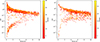 |
Fig. 2. Median period from their individual light curves and calculated ΔLS For all the 1950 M dwarf stars in the sample (left). Higher values of ΔLS indicate a greater spread in the values of the period over the sectors in which they were determined. The colours of the points indicate how many sectors of data were analysed. The same distribution but for the 1432 stars in our solar-like sample is shown on the right. |
We therefore use the approach of Lu et al. (2022), who determined the spread in the period in different quarters of Kepler data, using:

where NS is the number of sectors with measured PLS, s, and ⟨⋯⟩ denotes the median value operator. We do not necessarily expect the rotation period of active stars to be strictly periodic and therefore have very low values of ΔLS, since active regions can emerge and vanish at different latitudes over the sequence of the observations, which together with differential rotation of the star can lead to slightly different observed periods.
Since the LSP can identify half the real period when pulse profiles are double peaked, we determined the median period and ΔLS and then recomputed ΔLS so that if an individual sector was half the median period (within a few percent) we used twice this value and redetermined ΔLS. We show the median period and its spread (ΔLS) for all 1950 stars in the left hand panel of Figure 2. There are two clear grouping: a band of points starting at the lower left which have very low ΔLS values that progress to higher values as the period increases. A second group of points starts in the top left hand corner which have a large spread in ΔLS, which decreases as the period increases.
We examined the light curves and periodograms for stars which had median periods shorter than 2 d but had values of ΔLS higher than the strip of sources with low ΔLS: we found evidence for some stars appearing to be pulsators and others that had a longer period modulation super-imposed on the shorter period seen in an earlier cycle of observations. This suggests that at least some stars above the band of stars seen in the low ΔLS strip are probably real variable stars, but not isolated single M dwarfs which have starspots. Of course many others are likely not real variable stars and the LSP has just picked random peaks in the power spectrum, which are likely due to red noise.
We now make a comparison with the solar-like sample discussed in Sect. 3. We applied exactly the same procedures as we did for the M dwarf sample. Given solar-type stars are expected to show (in general) rotation periods much longer than a few days (e.g. McQuillan et al. 2014), we would not expect to see the same band of points at the lower left – unless their periods were spurious. We show the distribution of the 1432 solar-type stars in the right hand panel of Figure 2: we find the same spread of points with high ΔLS, but only a few stars in the lower left. There are 17 solar-like stars which appear to show very stable periods (Figure 2). We searched the SIMBAD1 database for information on these stars and found they were a mixture of eclipsing binaries; eruptive variables and red clump low-mass core He-burning stars (e.g. Ruiz-Dern et al. 2018). We conclude they are not single solar-like pulsator stars, but other types of variable star instead; this lends support to the view that the majority of stable periodic low-mass stars (left-hand panel of Figure 2) are single low-mass stars that have long-lived starspots.
In selecting those sources with which to search for changes in the amplitude of variability, we observe that in both samples, there is a ‘natural’ split between most sources, with ΔLS > 0.05 and ΔLS < 0.05. We therefore identified 245/1950 M dwarfs and 194/1432 solar-type stars which have ΔLS < 0.05 for the next stage of our analysis.
 |
Fig. 3. Three examples of low-mass stars, TIC 142015852, TIC 160118032, and TIC 441811894, which have a variable rotational amplitude. |
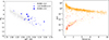 |
Fig. 4. Gaia HRD (BP − RP, MG) of low mass stars (grey) with those identified as showing significant variability of the rotational amplitude over time shown as circles whose size indicates their Gaia RUWE value (see text for details) on the left. The low mass star sample (orange dots) is on the right-hand panel, with the 29 stars which were identified as having a rotational amplitude which varies significantly over time shown as a red × symbol. |
4. Searching for variations in the rotational amplitude
Since the number of amplitude measurements per star is small (a maximum of 30 spread over five years) we need to identify a suitable statistical test which can robustly identify variations or trends in the data. To achieve this, we have used two different non-parametric tests for variability in the time series, namely, the Mann-Kendall (MK) test for monotonic trends in time series (Mann 1945; Kendall 1975) and a modified (non-parametric) version of the R-statistic introduced in Baptista & Steiner (1993). The MK test is sensitive to monotonic (both linear and non-linear) trends in the data, whilst the Rnp-test measures the temporal distribution of the signs of the residuals, ri, after subtracting the mean level from the time series. We define Rnp as:

where ri are the time series residuals after subtracting the mean level. Then Rnp follows a discrete normal distribution with a mean 0.0 and σ = 1.0. Large positive values of Rnp correspond to cases where a number of consecutive datapoints show the same sign (either + or –) in their residuals after subtraction of the mean, namely, the constant value model does not fit the data. The large negative values of Rnp would imply systematically alternating consecutive residuals with opposite signs and could only arise if the data contained a short period that roughly matches the sampling period. This case is not relevant here. The probability distribution for Rnp is discrete Gaussian, even if the data distribution would not be known. This enables us to obtain reliable probabilities for Rnp values, even in the case of a small number of points.
These two tests are sensitive to different types of variability (monotonic trend vs correlated and systematic residuals for a constant model) that can be present in the data. We therefore selected those stars whose amplitude variation over time gave a FAP < 0.0001 with either the MK stat or the Rnp-stat and had a minimum of 6 data points: this resulted in 29 low-mass stars (if we choose FAP < 0.001, we obtain 53 stars). The details of these 29 stars are shown in Table 1 with three example light curves showing the amplitude variation over time is shown in Figure 3 (the amplitude variation of all 29 stars are shown in Figures A.1–A.3). There is a range of light curve characteristics such as TIC 142015852 which shows a rise to maximum followed by a dip 1.5 yrs later; TIC 160118032 which shows a continuous increase amplitude over three yrs and TIC 441811894, which shows a rise followed by a decline several years later. In contrast, we found evidence for only one star in our solar-like sample (TIC 38707949) that showed a general decrease in rotational amplitude over a timescale of 2.5 yrs.
Details of the 29 low mass stars which show a significant variability in their rotational amplitude over time.
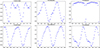 |
Fig. 5. First sector of data for six stars in our M dwarf sample which have been folded and binned on the period of the highest peak in the LSP: the phase is arbitrary. The left-hand and middle stars in the upper panel are in the binary sample of Penoyre et al. (2022), while TIC 38586438 appears to be an eclipsing binary. The shape of the folded light curves of TIC 160118032, 271693722 and 142082942 are representative of other stars in the sample. |
We also show the 29 stars in the Gaia HRD in the left-hand panel of Figure 4, which shows that they are biased towards the red or more luminuous parts of the lower main sequence. This may imply the stars are younger compared to the overall sample or they are members of binaries. To explore this further, we indicate using the colour of the points the Gaia renormalised unit weight error (RUWE) parameter for each of the 29 stars. This is a measure of how much the photo-center of a star moves over the course of the Gaia observations (Lindegren 2021a). Initial indications suggest that for stars with RUWE > 1.4 the star is an unresolved binary system (Lindegren 2021b), although this does not preclude that binaries can have RUWE values < 1.4 (Stassun & Torres 2021) and that the distribution of RUWE can vary over the Gaia HRD (Penoyre et al. 2022). We cross matched our 29 low-mass stars with the resulting catalogue of binaries within 100 pc from Penoyre et al. (2022), finding that only two sources with the highest RUWE (> 5.5) were in their catalogue. However, 7 out of these 29 stars exhibit RUWE > 1.4, suggesting they are possibly binary systems.
We folded and phase-binned the data on the period identified for that sector and we show six examples in Figure 5. Two of the stars were in the binary sample derived by Penoyre et al. (2022). Another one star, TIC 38586438, is an eclipsing binary. We show the folded light curves for three stars that are representative of the other stars in the sample.
In the right-hand panel of Figure 4, we show a similar plot as the left hand panel of Figure 2, but highlighting the location of the 29 low-mass stars that we identified as having variable amplitudes. Out of the 29 stars, 26 are located in the band of stars with low ΔLS values. All the stars have periods shorter than 7 days. There are three stars with periods shorter than 2 days and have ΔLS values much higher than the others. One of these (TIC 33881250) has one sector where the period of the highest peak differs from the others and has a much higher FAP, although several flares could have interfered with the period determination. Another two stars (TIC 149347629 and 441811894) show two periods with the highest peak changing: this may indicate they are pulsators. Therefore, we did not consider these stars in the next stage of the analysis and, thus, we were left with 26 stars.
5. Expected length of stellar cycles in low-mass stars
Using measurements of the Ca II H&K lines using data taken at Mt Wilson from the 1960s (Wilson 1968), Brandenburg et al. (1998) found evidence that the ratio of the period of the activity cycle, Pcyc, and the stellar rotation period, Prot, was related to the Rossby number (Ro = Prot/τ), where τ is the convective turnover time. More recently, Irving et al. (2023) searched for a relationship between Pcyc/Prot and Ro for solar-like and M dwarf stars. For the latter, they determined Pcyc/Prot = 3.6 R (see Fig. 16 and Eq. 4 of Irving et al. 2023). Based on this relationship, we calculated what the predicted Pcyc for the stars in our sample would be. We assume that the period we measured from the TESS data is the star’s rotation period.
Because Ro is not an observable quantity, we have to use a proxy. One established means is the one derived by Wright et al. (2018), who use the (V − Ks) colour to derive τ. However, Irving et al. (2023) using work of Corsaro et al. (2021), Landin et al. (2023) and Pecaut & Mamajek (2013) derived new relationships for (V − Ks) and τ. For (V − Ks) < 4.6 (stars earlier than M3V), the resulting values of τ are similar to that of Wright et al. (2018). Following Irving et al. (2023), we used the τL relationship for (V − Ks) < 4.6 and τG for (V − Ks) > 4.6 (see Figure 13 of Irving et al. 2023: for those stars near the boundary we chose the higher value). The values of τ for each star are shown in Table 1. Using τ and the period for each star, we computed Ro and used the relationship of Irving et al. between Pcyc/Prot and Ro to determine the length of the activity cycle of our stars. We show the predicted cycle lengths in Table 1 which range from 0.6–4.6 yrs: they are longer by a factor of ∼2–7 compared to the values determined by simply using the relationship of Wright et al. (2018).
The amplitude variation over time is shown for all stars in Figures A.1 and A.3. To estimate the length of the activity cycles from the amplitude time series data, we experimented with fitting the amplitude time series with a Fourier series models with different number of harmonic terms and also the period as a free parameter. Such a problem is non-linear and, thus, we carried out extensive MCMC fitting to derive the limits and the probability distribution for any activity periods. However, we were not able to obtain repeatable and reliable results. This is due to the gaps in the time series and the length of the trends. However, it is clear that some stars such as TIC 441734910 have a downward trend lasting ∼3.5 yrs, implying any activity cycles could be ∼8–10 yrs. The predicted activity cycle based on the relationship of Irving et al. (2023) is 7.2 yrs. In contrast, TIC 142015852 shows an amplitude variation which is consistent with a timescale of ∼3 yrs: the predicted cycle length is 1.3 yrs. This gives us modest confidence that the variations we observe are of the same order as the predicted timescales for activity cycles.
6. Amplitude variation as a function of rotation period
We determined the range in the amplitude over time by simply taking the difference between the maximum and minimum values for each of the 26 stars. The fractional mean amplitude (max-min) is 0.022, with a range between 0.005 and 0.063. We then searched for a correlation between the ‘max-min’ and the stars mass, temperature (from the TIC, Stassun & Torres 2021) and rotation period. We used the Kendall τ test to determine the significance of any correlation. We found no evidence for a correlation between mass or temperature. However, we found a FAP for the rank correlation between the amplitude variation and modulation period of 0.00587 (Figure 6). We note that a similar result was found when we compared the amplitude variation with Rossby number. Although this implies a 99.41 percent probability that the correlation is real, it does not formally reach the 3σ level. The one outlying point is TIC 341870349 (Prot∼4 d), although the reason behind this is not yet clear.
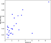 |
Fig. 6. Variation in the amplitude of the modulation over the course of their observation as a function of modulation period. There is a marginally significant trend in the rise of the amplitude variation over period. |
Although the statistical confidence in the correlation does not formally reach the 3σ level, we note that stars showing a larger range in the amplitude of modulation are likely to have a greater asymmetry in the distribution of spots than stars showing a smaller modulation. It may imply that stars that are faster rotating (and therefore likely to be young) have spots that are more uniformly distributed and cover a larger fraction of their photosphere.
7. Discussion
There is now robust evidence from spectroscopic observations that solar-like stars may exhibit stellar activity cycles that are similar in duration to those of the Sun. This is because of the length of observations, such as initiated at Mt Wilson (Wilson 1968), but also more recent high-precision spectroscopy from instruments such as HARPS (Lovis et al. 2011). Obtaining similarly robust claims for other stars such as M dwarfs using photometric measurements is difficult since all-sky precise photometry is still challenging (e.g. Stubbs & Tonry 2006). We also note that most claims of significant detections of periods in photometric data are made using the LSP, which assume that data have a Gaussian noise profile, whereas almost all such data streams contain red noise which result in FAPs which are far lower than they are in reality (e.g. Littlefair et al. 2017). Similarly, Basri & Shah (2020), using simulations of star spot distributions, show that ‘short’ activity cycles (of the order of several tens or more rotation cycles) are simply due to random processes.
In this exploratory study, we have gone to great lengths to identify stars that have very stable photometric periods over a timescale of several years. As a result, we have found 26 low-mass M dwarfs that show evidence for a significant variation in the amplitude of their rotational modulation over a time interval of nearly five years. There are some stars whose amplitude variation points to a long-term cycle of up to ten years and there are other stars whose timescale is ∼3–4 yrs. Given the relatively short rotation periods, we do not consider these to be equivalent to the spurious activity cycles noted by Basri & Shah (2020).
Compared to solar-like stars, the number of low-mass stars (MV and later) that have robustly determined activity cycles from spectra is much fewer, partly because they are fainter in the blue, which is where the activity marker Ca II H&K lines are present. Suárez Mascareño et al. (2016) used photometric data obtained using the All Sky Automated Survey (ASAS) to search for activity cycles and found 25 early M and 9 mid M spectral types; these samples were biased towards relatively long rotational periods, a median of 33.4 d (early M) and 86.2 d (mid M). In the sample of Irving et al. (2023) mentioned in Sect. 5, of their 15 stars, four had periods shorter than 6 d, and there was only one with a period shorter than 2 d. Our sample of 26 stars therefore reveals a set of low-mass stars that are rapidly rotating and have potential activity cycles.
8. Conclusion
In this pilot study, we have examined the TESS light curves of 1950 low-mass and 1432 solar-type stars. We found that only 245 (12.6%) low-mass stars showed stable periods over many sectors compared to 194 (13.5%) solar-type stars. Thus, we assume that these periods are a signature of the stars rotation period. However, there are many more low-mass stars which show very stable periods at periods shorter than ∼4 d than solar-type stars. This implies that the low spread in the measured periods of the short period M dwarfs is real and not produced by sampling or any artefacts in the data. We note that the FAP of periods detected using the LSP can give periods that may appear to be significant at the 1% level (commonly used in the literature), but that are, in fact, due to red noise.
We searched for variations in the amplitude of the rotation period using two statistical tests and found that 29 low-mass stars and one solar-type star shows evidence for significant variability. The TESS light curves of stars in the continuous viewing zones all have gaps of one year. This makes determining any meaningful estimate of the period of variation difficult. However, they are not widely inconsistent with the predicted cycle length, which is based on the stars Rossby number.
One mission which will observe the same field continuously is ESA’s PLATO mission, which is due to be launched in Dec. 2026 and will make an initial pointing in the southern hemisphere lasting at least 2 yrs (Nascimbeni et al. 2022), covering a continuous area of 1037 deg2. Since this field will have been observed a number of times using TESS, it will provide the means to study the modulation amplitude of thousands of stars over a time interval that is comparable or longer to the expected activity cycles.
Another means to fill the gaps is ground based wide-field optical surveys such as GOTO (Steeghs et al. 2022; Dyer et al. 2022) or ATLAS (Tonry et al. 2018), which have telescopes in both hemispheres that are perfectly placed to fill in the gaps when TESS is not able to observe parts of the sky. In that case, they can make extended observations of the same fields every few months. It would also be interesting to determine if there is any variation in the X-ray flux of the 26 stars found to show long-term variability in their rotational amplitude. We hope that eRosita (Predehl et al. 2021) will be able to resume operations in the near future.
Acknowledgments
This paper includes data collected by the TESS mission, for which funding is provided by the NASA Explorer Program. This work also presents results from the European Space Agency (ESA) space mission Gaia. Gaia data is being processed by the Gaia Data Processing and Analysis Consortium (DPAC). Funding for the DPAC is provided by national institutions, in particular the institutions participating in the Gaia MultiLateral Agreement (MLA). The Gaia mission website is https://www.cosmos.esa.int/gaia. The Gaia archive website is https://archives.esac.esa.int/gaia. Armagh Observatory & Planetarium is core funded by the N. Ireland Executive through the Dept. for Communities. JGD would like to thank the Leverhulme Trust for a Emeritus Fellowship.
References
- Anthony, F., Núñez, A., Agüeros, M. A., et al. 2022, AJ, 163, 257 [NASA ADS] [CrossRef] [Google Scholar]
- Baliunas, S. L., Donahue, R. A., Soon, W. H., et al. 1995, ApJ, 438, 269 [Google Scholar]
- Baptista, R., & Steiner, J. E. 1993, A&A, 277, 331 [NASA ADS] [Google Scholar]
- Basri, G., & Shah, R. 2020, ApJ, 901, 14 [Google Scholar]
- Berdyugina, S. V., & Järvinen, S. P. 2005, Astron. Nachr, 326, 283 [CrossRef] [Google Scholar]
- Brandenburg, A., Saar, S. H., & Turpin, C. R. 1998, ApJ, 498, L51 [NASA ADS] [CrossRef] [Google Scholar]
- Caldwell, D. A. 2020, RNAAS, 4, 201 [NASA ADS] [Google Scholar]
- Corsaro, E., Bonanno, A., Mathur, S., et al. 2021, A&A, 652, L2 [NASA ADS] [CrossRef] [EDP Sciences] [Google Scholar]
- Davenport, J. R. A. 2016, ApJ, 829, 23 [Google Scholar]
- Dorn-Wallenstein, T. Z., Levesque, E. M., & Davenport, J. R. A. 2019, ApJ, 878, 155 [NASA ADS] [CrossRef] [Google Scholar]
- Doyle, J. G., Butler, C. J., Callanan, P. J., et al. 1988a, A&A, 191, 79 [NASA ADS] [Google Scholar]
- Doyle, J. G., Butler, C. J., Byrne, P. B., & van den Oord, G. H. J. 1988b, A&A, 193, 229 [NASA ADS] [Google Scholar]
- Doyle, J. G., Mathioudakis, M., Murphy, H. M., et al. 1993, A&A, 278, 499 [NASA ADS] [Google Scholar]
- Dyer, M. J., Ackley, K., Lyman, J., et al. 2022, SPIE, 12182, 121821 [Google Scholar]
- Hartman, J. D., & Bakos, G. Á. 2016, Astron. Comput., 17, 1 [Google Scholar]
- Henry, T. J., Jao, W.-C., Subasavage, J. P., et al. 2006, AJ, 132, 2360 [Google Scholar]
- Ibañez Bustos, R. V., Buccino, A. P., Messina, S., & Lanza, A. F. 2020, A&A, 644, A2 [NASA ADS] [CrossRef] [EDP Sciences] [Google Scholar]
- Irving, Z. A., Saar, S. H., Wargelin, B. J., & do Nascimento, J. D. 2023, ApJ, 949, 51 [NASA ADS] [CrossRef] [Google Scholar]
- Jackson, R. J., & Jeffries, R. D. 2013, MNRAS, 431, 1833 [Google Scholar]
- Jeffers, S. V., Kiefer, R., & Metcalfe, T. S. 2023, Space Sci. Rev., 219, 54 [CrossRef] [Google Scholar]
- Kendall, M. G. 1975, Rank Correlation Methods, 4th edn. (London: Charles Griffin) [Google Scholar]
- Konings, T., Baeyens, R., & Decin, L. 2022, A&A, 667, A15 [NASA ADS] [CrossRef] [EDP Sciences] [Google Scholar]
- Küker, M., Rüdiger, G., Olah, K., & Strassmeier, K. G. 2019, A&A, 622, A40 [NASA ADS] [CrossRef] [EDP Sciences] [Google Scholar]
- Landin, N. R., Mendes, L. T. S., Vaz, L. P. R., & Alencar, S. H. P. 2023, MNRAS, 519, 5304 [NASA ADS] [CrossRef] [Google Scholar]
- Lindegren, L. 2021a, A&A, 649, A2 [NASA ADS] [CrossRef] [EDP Sciences] [Google Scholar]
- Lindegren, L. 2021b, A&A, 649, A4 [NASA ADS] [CrossRef] [EDP Sciences] [Google Scholar]
- Littlefair, S. P., Burningham, B., & Helling, C. 2017, MNRAS, 466, 4250 [NASA ADS] [Google Scholar]
- Lovis, C., Dumusque, X., Santos, N. C., et al. 2011, arXiv e-prints [arXiv:1107.5325] [Google Scholar]
- Lu, Y., Benomar, O., Kamiaka, S., & Suto, Y. 2022, ApJ, 941, 175 [NASA ADS] [CrossRef] [Google Scholar]
- Luger, R., Foreman-Mackey, D., Hedges, C., & Hogg, D. W. 2021a, AJ, 162, 123 [NASA ADS] [CrossRef] [Google Scholar]
- Luger, R., Foreman-Mackey, D., Hedges, C., & Hogg, D. W. 2021b, AJ, 162, 124 [NASA ADS] [CrossRef] [Google Scholar]
- Mann, H. B. 1945, Econometrica, 13, 163 [Google Scholar]
- McQuillan, A., Mazeh, T., & Aigrain, S. 2014, ApJS, 211, 24 [Google Scholar]
- Nascimbeni, V., Piotto, G., Börner, A., et al. 2022, A&A, 658, A31 [NASA ADS] [CrossRef] [EDP Sciences] [Google Scholar]
- Pecaut, M. J., & Mamajek, E. E. 2013, ApJS, 208, 9 [Google Scholar]
- Penoyre, Z., Belokurov, V., & Evans, N. W. 2022, MNRAS, 513, 5270 [Google Scholar]
- Pettersen, B. R. 1989, Sol. Phys., 121, 299 [NASA ADS] [CrossRef] [Google Scholar]
- Predehl, P., Andritschke, R., Arefiev, V., et al. 2021, A&A, 647, A1 [EDP Sciences] [Google Scholar]
- Rebull, L. M., Padgett, D. L., McCabe, C. E., et al. 2016, AJ, 152, 113 [NASA ADS] [CrossRef] [Google Scholar]
- Reinhold, T., Cameron, R. H., & Gizon, L. 2017, A&A, 602, A52 [NASA ADS] [CrossRef] [EDP Sciences] [Google Scholar]
- Ricker, G., Winn, J. N., Vanderspek, R., et al. 2015, J. Astron. Telescopes Instrum. Syst., 1, 014003 [Google Scholar]
- Rodono, M., Cutispoto, G., Pazzani, V., et al. 1986, A&A, 165, 135 [NASA ADS] [Google Scholar]
- Ruiz-Dern, L., Babusiaux, C., Arenou, F., Turon, C., & Lallement, R. 2018, A&A, 609, A116 [NASA ADS] [CrossRef] [EDP Sciences] [Google Scholar]
- Smart, R. L., Sarro, L. M., Rybizki, J., et al. 2021, A&A, 649, A6 [Google Scholar]
- Stassun, K., Oelkers, R. J., Pepper, J., et al. 2018, AJ, 156, 102 [NASA ADS] [CrossRef] [Google Scholar]
- Stassun, K. G., & Torres, G. 2021, ApJ, 907, L33 [NASA ADS] [CrossRef] [Google Scholar]
- Steeghs, D., Galloway, D. K., Ackley, K., et al. 2022, MNRAS, 511, 2405 [NASA ADS] [CrossRef] [Google Scholar]
- Stubbs, C. W., & Tonry, J. L. 2006, ApJ, 646, 1436 [NASA ADS] [CrossRef] [Google Scholar]
- Suárez Mascareño, A., Rebolo, R., & González Hernández, J. I. 2016, A&A, 595, A12 [Google Scholar]
- Tonry, J. L., Denneau, L., Heinze, A. N., et al. 2018, PASP, 130, 064505 [Google Scholar]
- Wargelin, B. J., Saar, S. H., Pojmański, G., Drake, J. J., & Kashyap, V. L. 2017, MNRAS, 464, 3281 [NASA ADS] [CrossRef] [Google Scholar]
- Wilson, O. C. 1968, ApJ, 153, 221 [Google Scholar]
- Wright, N. J., Newton, E. R., Williams, P. K. G., Drake, J. R., & Yadav, R. K. 2018, MNRAS, 479, 2351 [NASA ADS] [CrossRef] [Google Scholar]
- Zechmeister, M., & Kürster, M. 2009, A&A, 496, 577 [CrossRef] [EDP Sciences] [Google Scholar]
Appendix A: Long-term variability in the amplitude
 |
Fig. A.1. Amplitude of the rotational modulation of low-mass stars that we have identified as showing significant variability. |
 |
Fig. A.2. Amplitude of the rotational modulation of low-mass stars that we have identified as showing significant variability (cont). |
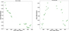 |
Fig. A.3. Amplitude of the rotational modulation of low-mass stars that we have identified as showing significant variability (cont). |
All Tables
Details of the 29 low mass stars which show a significant variability in their rotational amplitude over time.
All Figures
|
Fig. 1. Gaia HRD (BP − RP, MG) of low-mass stars (red) and solar type stars (green) that were observed for at least six sectors in each TESS Cycle. |
| In the text | |
|
Fig. 2. Median period from their individual light curves and calculated ΔLS For all the 1950 M dwarf stars in the sample (left). Higher values of ΔLS indicate a greater spread in the values of the period over the sectors in which they were determined. The colours of the points indicate how many sectors of data were analysed. The same distribution but for the 1432 stars in our solar-like sample is shown on the right. |
| In the text | |
|
Fig. 3. Three examples of low-mass stars, TIC 142015852, TIC 160118032, and TIC 441811894, which have a variable rotational amplitude. |
| In the text | |
|
Fig. 4. Gaia HRD (BP − RP, MG) of low mass stars (grey) with those identified as showing significant variability of the rotational amplitude over time shown as circles whose size indicates their Gaia RUWE value (see text for details) on the left. The low mass star sample (orange dots) is on the right-hand panel, with the 29 stars which were identified as having a rotational amplitude which varies significantly over time shown as a red × symbol. |
| In the text | |
|
Fig. 5. First sector of data for six stars in our M dwarf sample which have been folded and binned on the period of the highest peak in the LSP: the phase is arbitrary. The left-hand and middle stars in the upper panel are in the binary sample of Penoyre et al. (2022), while TIC 38586438 appears to be an eclipsing binary. The shape of the folded light curves of TIC 160118032, 271693722 and 142082942 are representative of other stars in the sample. |
| In the text | |
|
Fig. 6. Variation in the amplitude of the modulation over the course of their observation as a function of modulation period. There is a marginally significant trend in the rise of the amplitude variation over period. |
| In the text | |
|
Fig. A.1. Amplitude of the rotational modulation of low-mass stars that we have identified as showing significant variability. |
| In the text | |
|
Fig. A.2. Amplitude of the rotational modulation of low-mass stars that we have identified as showing significant variability (cont). |
| In the text | |
|
Fig. A.3. Amplitude of the rotational modulation of low-mass stars that we have identified as showing significant variability (cont). |
| In the text | |
Current usage metrics show cumulative count of Article Views (full-text article views including HTML views, PDF and ePub downloads, according to the available data) and Abstracts Views on Vision4Press platform.
Data correspond to usage on the plateform after 2015. The current usage metrics is available 48-96 hours after online publication and is updated daily on week days.
Initial download of the metrics may take a while.