| Issue |
A&A
Volume 689, September 2024
|
|
|---|---|---|
| Article Number | A283 | |
| Number of page(s) | 10 | |
| Section | Extragalactic astronomy | |
| DOI | https://doi.org/10.1051/0004-6361/202449626 | |
| Published online | 19 September 2024 | |
ALMA reveals a dust-obscured galaxy merger at cosmic noon
1
European southern Observatory, Karl-Schwarzschild-Str. 2, 85748 Garching, Germany
2
Univ Lyon, Univ Lyon1, Ens de Lyon, CNRS, Centre de Recherche Astrophysique de Lyon (CRAL) UMR5574, 69230 Saint-Genis-Laval, France
3
Dipartimento di Fisica e Astronomia, Università di Firenze, Via G. Sansone 1, 50019 Sesto Fiorentino (Firenze), Italy
4
INAF – Osservatorio Astrofisico di Arcetri, Largo E. Fermi 5, 50125 Firenze, Italy
5
University of Bologna – Department of Physics and Astronomy “Augusto Righi” (DIFA), Via Gobetti 93/2, 40129 Bologna, Italy
6
INAF – Osservatorio Astrofisico e Scienza della Spazio, Via Gobetti 93/3, 40129 Bologna, Italy
7
Cosmic Dawn Center (DAWN), Copenhagen, Denmark
Received:
15
February
2024
Accepted:
31
May
2024
Abstract
Context. Galaxy mergers play a critical role in galaxy evolution. They alter the size, morphology, dynamics, and composition of galaxies. Galaxy mergers have so far mostly been identified through visual inspection of their rest-frame optical and near-IR (NIR) emission. Dust can obscure this emission, however, resulting in the misclassification of mergers as single galaxies and in an incorrect interpretation of their baryonic properties.
Aims. Having serendipitously discovered a dust-obscured galaxy merger at z = 1.17, we aim to determine the baryonic properties of the two merging galaxies, including the star formation rate (SFR) and the stellar, molecular gas and dust masses.
Methods. Using Band 3 and 6 observations from the Atacama Large Millimeter and submillimeter Array (ALMA) and ancillary data, we studied the morphology of this previously misclassified merger. We deblended the emission, derived the gas masses from CO observations, and modeled the spectral energy distributions to determine the properties of each galaxy. Using the rare combination of ALMA CO(2–1), CO(5–4) and dust-continuum (rest-frame 520 μm) observations, we provide insight into the gas and dust content and into the properties of the interstellar medium of each merger component.
Results. We find that only one of the two galaxies is highly obscured by dust, but both are massive (> 1010.5 M⊙) and highly star forming (SFR = 60 − 900 M⊙/yr), have a moderate-to-short depletion time (tdepl < 0.7 Gyr) and a high gas fraction (fgas ≥ 1).
Conclusions. These properties can be interpreted as the positive impact of the merger. With this serendipitous discovery, we highlight the power of (sub)millimeter observations to identify and characterise the individual components of obscured galaxy mergers.
Key words: dust / extinction / galaxies: evolution / galaxies: high-redshift / galaxies: interactions / galaxies: ISM / galaxies: star formation
Corresponding author; This email address is being protected from spambots. You need JavaScript enabled to view it. .
© The Authors 2024
 Open Access article, published by EDP Sciences, under the terms of the Creative Commons Attribution License (https://creativecommons.org/licenses/by/4.0), which permits unrestricted use, distribution, and reproduction in any medium, provided the original work is properly cited.
This article is published in open access under the Subscribe to Open model. This email address is being protected from spambots. You need JavaScript enabled to view it. to support open access publication.
1. Introduction
Throughout their evolution, galaxies can encounter one or more companions closely enough for the gravitational interaction to pull them together in galaxy mergers. During galaxy mergers, the evolution of galaxies is driven by turbulent and stochastic processes. This can dramatically affect the properties of galaxies on many levels, including star formation (e.g. Ellison et al. 2022), active galactic nuclei (AGN) activity (e.g. Byrne-Mamahit et al. 2023) and morphology (e.g. Martin et al. 2018). In particular, mergers can entrain gas to the centre of galaxies by breaking the angular momemtum of the accreting gas, which may result in a higher star formation than in typically star-forming galaxies (SFGs) on the main sequence (MS; e.g. Kim et al. 2009; Saitoh et al. 2009; Kaviraj et al. 2015; Tacchella et al. 2016; Pearson et al. 2019).
Merger rates appear to increase as a function of redshift (e.g. Ventou et al. 2019; Romano et al. 2021; Conselice et al. 2022; Ren et al. 2023). In the local Universe, close to 1% of the galaxies with similar masses (i.e. major mergers) are merging, while the fraction increases to just below 20% at cosmic noon, that is, z = 1 − 2, where the Universe is most active and reaches its star formation peak (e.g. Madau & Dickinson 2014 and references therein). Based on a visual classification from rest-frame V-band Hubble Space Telescope (HST) imaging, Kaviraj et al. (2013) found that major mergers contribute up to 27% to the star formation activity at the start of cosmic noon, that is, z ∼ 2. Furthermore, galaxy mergers are a unique laboratory for studying the different processes involved in the evolution of galaxies because they bridge a wide range of physical scales from star formation (e.g. enhancement of star formation due to gas and dust compression at subparsec scales) to large-scale structures (galaxy clustering at megaparsec scales).
Galaxy mergers are key to understanding the evolution of galaxies. However, it remains a challenge to accurately identify them all. In works based on observations (e.g. Mundy et al. 2017; Ren et al. 2023), the common method for identifying galaxies as mergers is to visually inspect rest-frame optical or near-IR (NIR) data using telescopes such as the HST, with a set of selection criteria based on spatial and velocity separations to ensure that the galaxies are gravitationally bound. Typically, galaxies are selected from rest-frame optical or NIR data to lie within a few dozen kiloparsec of each other or with a relative velocity lower than a few hundreds of km s−1 (e.g. Lotz et al. 2008; Casteels et al. 2014; Ventou et al. 2019). The common method described above implies that we are able to identify all the galaxies that are part of merging systems to classify systems as such, using rest-frame optical or NIR data alone. However, at z ∼ 1 − 2, nearly 70% of the ongoing star formation is in an obscured phase (Zavala et al. 2021). This can result in obscured galaxies being missed when only rest-optical observations are used. For instance, Talia et al. (2021), Enia et al. (2022), Behiri et al. (2023), Smail et al. (2023), and Gentile et al. (2023) found dusty star-forming galaxies (DSFGs) that appeared to be optically dark because dust obscured the emission at rest-frame optical wavelengths. Galaxy mergers could thus be missed by classical merger identification approaches because one or several members of the merger can originally (i.e. before the mergering phase) be dusty or because the merger itself drives up the build-up of a large dust reservoir. If such optically dark mergers exist, they might be observed at longer wavelength, that is, in the mid-infrared (MIR) to (sub)millimeter wavelengths, where obscuring dust does not limit the observations. With the advance of telescopes capable of observing at these longer wavelengths and reaching high angular resolution, such as the Atacama Large Millimeter and submillimeter Array (ALMA), we can thus reveal very complex systems that were otherwise hidden by dust. These systems represent unique laboratories to further our understanding of the baryonic properties of galaxies. In particular, CO observations with an angular resolution that is sufficient to distinguish merger members provide us with a window into the molecular gas and dust content of individual galaxies in mergers at cosmic noon. Thus, (sub)millimeter observations improve the characterisation of mergers by adding information that is otherwise not accessible at shorter wavelengths (e.g. in the NIR).
Using ALMA archival observations, we present the serendipitous detection of a system within the Cosmic Evolution Survey (COSMOS; Scoville et al. 2007) field consisting of two massive merging galaxies at z ∼ 1. This system was previously misclassified as a single source (COSMOS-51599) because one of the two galaxies is optically dark, that is, no emission is apparent in the HST WFC3/UVIS F814W observations (COSMOS super-deblended catalogue; Jin et al. 2018) in the COSMOS2020 catalogue (Weaver et al. 2022). We use ALMA archival observations to reveal an additional galaxy, indicating the presence of a previously missed merger system (which we refer to as Matilda1). We use the archival ALMA CO(2–1), CO(5–4) and dust continuum observations to study the gas and dust content and the physical conditions of the interstellar medium (ISM) of the two galaxies involved in the merger.
This paper is organised as follows. In Section 2, we present the observations and data reduction. In Section 3, we describe how we identified the system and how we derived the baryonic properties of each galaxy. In Section 4, we discuss the results and their implications. We summarise our findings in Section 5. The cosmology assumed throughout this work follows the ΛCDM standard cosmological parameters: H0 = 70km s−1 Mpc−1, Ωm = 0.3, and ΩΛ = 0.7 (Planck Collaboration VI 2020). We use a Chabrier (2003) stellar initial mass function (IMF).
2. Multi-wavelength observations and data reduction
2.1. ALMA
We used the calibrated raw visibility data from the observations of programmes 2015.1.00260.S and 2016.1.00171.S (PI: Daddi), provided by the European ALMA Regional Centre (Hatziminaoglou et al. 2015). These two programmes include observations of Matilda (COSMOS-51599) at RA 09:58:23.630 and Dec +02:12:01.660 in Band 3 (2.6 − 3.6 mm) and Band 6 (1.1 − 1.4 mm), corresponding to CO(2–1), CO(5–4) and the dust continuum. Matilda is part of a sample of galaxies presented in Valentino et al. (2020), and we refer to that work for more details about the design of the survey and the associated observations.
We used the Common Astronomy Software Applications (CASA) data processing software (CASA Team 2022) throughout the analysis of the ALMA data. For the CO(2–1) observations, we performed uv-plane continuum subtraction (with uvcontsub) and imaged the CO(2–1) emission with natural weighting and with a channel width of Δv = 75 km s−1 (with tclean). This imaging step resulted in a cleaned cube, with a sensitivity of 0.82 mJy/beam in channels of 75 km s−1, where the beam is 1.5″ × 1.3″. We also created the intensity map of the CO(2–1) emission (with immoments) by integrating between −575 km/s to +475 km/s (channels 55–69), where the line is clearly detected in a spectrum extracted from an aperture of 2″ that encompasses the entire system (see the left panel of Figure 1). For the CO(5–4) data, we repeated the same procedure, that is, we subtracted the continuum and imaged with the same set of parameters as for the CO(2–1) data. This yielded a CO(5–4) cube with a sensitivity of 0.81 mJy/beam in channels of 75 km s−1, where the beam is 0.8″ × 0.7″. To create the intensity map of the CO(5–4) emission, we integrated this emission from −605 km/s to +445 km/s (channels 38 to 52). We chose this range because the line is clearly detected in a spectrum that is extracted with the same 2″ aperture as for the CO(2–1) emission (see the right panel of Figure 1). We imaged the continuum from the Band 6 data, excluding the region that covers the CO(5–4) line. This resulted in a continuum image with a sensitivity of 0.23 mJy/beam, where the beam is 0.8″ × 0.7″. All the intensity maps are shown in Figure 2. The CO(2–1), CO(5–4), and continuum emissions are clearly detected with a peak signal-to-noise ratio of 6, 6, and 14, respectively.
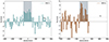 |
Fig. 1. CO(2–1) (left) and CO(5–4) (right) emissions of the entire system in mJy per 75 km/s as a function of the velocity, where the centre velocity is determined from the redshift z = 1.17. The channels used to create the intensity maps are highlighted with the grey shaded area. |
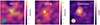 |
Fig. 2. Intensity maps (7″ × 7″) of the CO(2–1) emission (left) with [3, 4, 5, 6] σCO(2 − 1) contours, the CO(5–4) emission (middle) with [3, 4, 5, 6] σCO(5 − 4) contours, and the dust-continuum image (right) with [3, 5, 7, 9, 11] σdust contours. |
2.2. Other observations
Because our target is in the COSMOS field (Scoville et al. 2007), multi-wavelength ancillary data are already available. We used the ancillary photometric images available for our target through the IRSA COSMOS cutout service2, including Subaru/Hyper suprime-cam (HSC) data in the g, r, z, and y filters (Aihara et al. 2019), Visible and Infrared Survey Telescope for Astronomy (VISTA) data in the Y, J, H, and Ks filters (McCracken et al. 2012), HST/Wide field camera (WFC) in the F814W filter (Koekemoer et al. 2007; Massey et al. 2010), Spitzer/Infrared array camera (IRAC) in all channels (Euclid Collaboration 2022), and VLA at 3 GHz (10 cm) observations (Smolčić et al. 2017). We note that Weaver et al. (2022) astrometrically corrected all data sets based on Gaia DR2 (Gaia Collaboration 2018), that is, the HST data are aligned with the other data sets. Similarly, the ALMA observations are astrometrically aligned with the other data sets with an offset of up to 23 mas (Section 10.5.2 of Cortes et al. (2023)). This offset is negligible compared to the beam size of the observations used in this work (0.8″ in the case of the CO(5–4) observations, and 2″ in the case of the CO(2–1) observations).
3. Analysis of the data
3.1. Identification of the dusty galaxy merger
As shown in Figure 2, the CO(2–1) emission contours show an irregular morphology (i.e. inconsistent with a simple beam shape). The bulk of the emission is concentrated in the 6σ contours in the north, and a tail of fainter emission is located at 3 and 4σ towards the south. The CO(5–4) and dust-continuum contours also show a disturbed morphology (i.e. the emission extends in one direction beyond the beam shape), but are weaker than the CO(2–1) emission. We compare the extent of the CO(2–1) and dust-continuum emissions to the stellar emission traced by the HST/F814W data in Figure 3. The CO(2–1) emission extends beyond the HST/F814W emission, covering ∼2.6″ (i.e. ∼20 kpc), and it peaks where the emission in the HST/814W observations is low. An offset of the emission is also traced by ALMA, but not in the HST observations. The peak of the ALMA CO(2–1) emission is ∼1″ away from the peak in the HST emission. This corresponds to physical scales of 8kpc. We compared the extent and peak of the CO to the VISTA/Ks band, Spitzer/IRAC channel 2, and VLA/3 GHz observations (see Figure 4). The VISTA Ks-band observations, which trace old stellar populations, have two emission peaks. One peak coincides with the galaxy that is visible in the HST/F814W data (white contours), and the other peak coincides with the peak of the ALMA CO(2–1) and CO(5–4) emissions (only the ALMA CO(2–1) emission is shown for clarity with blue contours). In the Spitzer/IRAC channel 2 (4.5 μm) data, which also trace old stars, the point spread function (PSF) is too large to distinguish different components (see also Jin et al. 2018; Valentino et al. 2020). The VLA/3 GHz data, which trace high-energy sources such as active galactic nuclei (AGN) and star formation that is not biased by dust, are completely offset from the HST data, but are fully consistent with the peak of the ALMA data. This again confirms the presence of another galaxy that was missed in previous work. Thus, we conclude that we witness the merger of two galaxies at z = 1.17223 ± 0.00037 (Valentino et al. 2020). For the remainder of the paper, we call the northern component “North” (not visible in the HST/F814W data, bright in the VLA/3GHz data, and consistent with the peak of the ALMA data) and the southern component “South” (visible in the HST/F814W data and not visible in the VLA data).
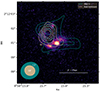 |
Fig. 3. HST F814W image from Koekemoer et al. (2007), with ALMA CO(2–1) contours in blue at [3, 4, 5, 6] σCO(2 − 1) and ALMA dust-continuum in beige at [3, 5, 7, 9, 11] σdust. The beams are shown in the lower left, with sizes of 1.3″ and 0.8″ for the CO(2–1) and dust-continuum emissions, respectively. A scale is shown at the bottom right to represent the physical scales at the redshift of the system, i.e., z = 1.17. |
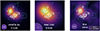 |
Fig. 4. ALMA CO(2–1) emission contours (in blue) and HST/F814W emission contours (in white) overlaid on Ultravista Ks band (left), IRAC channel 2 (middle), and VLA 10 cm (right) observations. These images are postage stamps of 5″ × 5″. |
3.2. Velocity and spatial offsets of the dusty galaxy merger
We imaged the velocity offset in the CO(2–1) and CO(5–4) emissions shown in Figure 1. We imaged the negative velocity peak (left column, solid lines in Figure 5) by integrating between −575 km/s and −50 km/s and the positive velocity peak (middle row, dash-dotted lines in Figure 5) by integrating between −50 km/s and +475 km/s for CO(2–1) and CO(5–4) (shown in the top and bottom row of Figure 5, respectively).
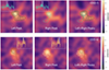 |
Fig. 5. Contours of the CO(2–1) (top row) and CO(5–4) (bottom row) intensity maps when integrating around the negative velocity peak (left column, solid lines) or the right peak (middle column, dash-dotted lines) of the emissions. The right column shows the two peaks overlaid. The negative and positive velocity peaks correspond to −575 km/s, −50 km/s, and −50 km/s to −475 km/s, respectively, for the CO(2–1) and CO(5–4) emissions. The contours start at 3σ and increase with an indent of 1σ. The background image in the top row (bottom row) is the CO(2–1) (CO(5–4)) emission when integrating the entire peak, as shown in the left (right) panel of Figure 2. The inset shows the spectrum, and the channels we used in the imaging are highlighted with the grey shaded area. |
As shown in the right panels of the top and bottom rows of Figure 5, North is traced by both peaks. In the CO(2–1) and the CO(5–4) emissions, the negative and positive velocity peaks are slightly shifted at the location of North. On the other hand, South seems to be traced by the negative velocity peak alone in the CO(2–1) and CO(5–4) emissions. Even though two clear peaks are observed in the CO(5–4) spectrum, no clear correspondence between one peak and its location in the imaging is visible when they are imaged separately, as shown in the bottom row of Figure 5, as might be expected if one peak represented one galaxy. The same applies for CO(2–1), but the distinction between the two peaks in the spectrum is less clear.
3.3. CO flux measurements
To separate the CO emission of the two galaxies that are part of the merger, we adopted the following deblending approach. We computed the CO(2–1) flux of the entire system within the 3σ contours shown in the left panel of Figure 2. This CO(2–1) intensity map shows bright emission within the size of a one-beam element centred on North. Therefore, we associated this bright component to North and estimated the CO(2–1) flux by measuring the flux within the single-beam element centred on North. The corresponding flux error is the standard deviation of the CO(2–1) intensity map, masking the emission of the merger (i.e. the emission within the 2″ used to extract the spectrum of the merger in Section 2.1). This resulted in FCO(2 − 1)north = 1.56 ± 0.25 Jy km/s. We associated the remaining emission within the CO(2–1) 3σ contours to South. This remaining emission was too faint, and we therefore used a 3σ upper limit, resulting in FCO(2 − 1)south ≤ 0.75 Jy km/s. With this method, we assumed that not all the gas that is associated with North belongs to South. There could be gas in between the two interacting galaxies, which would make this assumption incorrect. Because the resolution of the observations is limited, however, we were forced to make these simplifying assumptions. We performed this deblending method instead of using the PhoEBO (Gentile et al. 2023) code that we use in Section 3.6 because PhoEBO requires priors that are based on the position of the stellar emission, which we cannot assume to be aligned with the molecular gas and dust.
To derive the CO(5–4) fluxes of the two merging galaxies, we followed the same procedure. We associated the peak of the CO(5–4) emission within the 3σ contours of the CO(2–1) intensity map emission to North, resulting in FCO(5 − 4)north = 1.61 ± 0.24 Jy km/s, with the error being the standard deviation of the CO(5–4) intensity map (masking the emission coming from the merger within 2″). As for the CO(2–1) emission, the remaining CO(5–4) emission within the 3σ CO(2–1) contours was too faint, and therefore, we used a 3σ upper limit for the southern component, FCO(5 − 4)south ≤ 0.72 Jy km/s. We proceeded in the same way for the dust-continuum emission, finding Fcontnorth = 1.26 ± 0.09 mJy for North, and Fcontsouth ≤ 0.28 mJy for South.
3.4. Molecular gas masses from the CO(2–1) emission
We derived the molecular gas masses of the two galaxies by first converting the CO(2–1) fluxes into line luminosities via
 (1)
(1)
We converted the CO(2–1) luminosities into CO(1–0) luminosities assuming a ratio of 0.85 of the CO(2–1) and CO(1–0) luminosities (Carilli & Walter 2013). Then, we derived the molecular gas masses using the molecular gas-mass conversion factor αCO, with αCO = 3.4 ± 2 (K km s−1 p2)−1, which is the mean and standard deviation measured for a sample of z = 1 − 3 DSFGs in Harrington et al. (2021). The upper and lower errors on the molecular gas masses (see Table 1) reflect the uncertainty on αCO. We caution that the resulting molecular gas masses are highly dependent on the adopted αCO value. Lower values, for instance, αCO ∼ 0.9 as suggested in Bolatto et al. (2013) for starbursts, would result in five times lower molecular gas masses, which would also affect the results discussed in Section 4.2.
Properties of the individual components of the dusty major merger.
3.5. Excitation conditions of the molecular interstellar medium
We measure a CO(5–4) to CO(2–1) line ratio of FCO(5 − 4)/FCO(2 − 1) = 1.03 ± 0.35 for North. The flux measurements for South are upper limits, making FCO(5 − 4)/FCO(2 − 1) highly uncertain. We therefore omit the flux for this galaxy. The CO(5–4) to CO(2–1) ratio of North is similar to what Boogaard et al. (2020) reported for a stack of 22 SFGs at ⟨z⟩ = 1.2, that is, FCO(5 − 4)/FCO(2 − 1) = 1.41 ± 0.15. However, works on submillimeter galaxies (SMGs) at high redshift (z > 2) (e.g. Bothwell et al. 2013; Spilker et al. 2014) reported FCO(5 − 4)/FCO(2 − 1) > 2.4. In addition, Valentino et al. (2020) reported an increase in the CO(5–4) to CO(2–1) ratio with distance to the MS for a sample of a few dozen galaxies at ⟨z⟩ = 1.25, with FCO(5 − 4)/FCO(2 − 1) = 1.6 ± 0.2 for MS galaxies to FCO(5 − 4)/FCO(2 − 1) = 2.2 ± 0.3 for extreme starburst galaxies. Therefore, the ISM excitation conditions of North are similar to those of MS galaxies at similar redshift.
3.6. Stellar mass, dust mass, and star formation rate from a spectral energy distribution fitting
To measure the stellar mass, dust mass, and star formation rate (SFR), we separately modelled the spectral energy distributions (SEDs) of the two galaxies that we identified as part of the dusty galaxy merger by fitting the photometry with the SED-modelling tool called multi-wavelength analysis of galaxy physical properties (MAGPHYS; da Cunha et al. 2015; Battisti & Cunha 2020). However, we first had to deblend the two galaxies. The deblending is especially required for the Spitzer/IRAC observations, where the resolution is insufficient to distinguish the two galaxies.
We extracted the photometry of Matilda from the maps employed by Weaver et al. (2022) to assemble the COSMOS2020 catalogue. These data include the optical, NIR, and MIR maps from the Subaru/HSC, VISTA/VIRCAM, and Spitzer/IRAC instruments and telescope, respectively. To account for the significant source blending between the two components of this dusty galaxy merger, we used the tool called photometry extractor for blended objects (PhoEBO; Gentile et al. 2023). This code implements a slightly modified version of the algorithm introduced by Labbé et al. (2006) and has been employed in several studies (see e.g. Endsley et al. 2021; Whitler et al. 2023), but was optimized for the deblending of the so-called radio-selected NIR-dark galaxies (i.e. sources with a radio counterpart and no detection at optical/NIR wavelengths; e.g. Talia et al. 2021; Enia et al. 2022; Behiri et al. 2023; Gentile et al. 2023). PhoEBO deblended the two galaxies of which Matilda consists using a double prior coming from the high-resolution images in the radio and in the NIR bands, employing a PSF-matching with the low-resolution images (mainly those in the four IRAC channels) to attribute the flux to the different components in the analysed system. A detailed description of the code, available here3, can be found in Gentile et al. (2023). To measure the flux of the two deblended components, we performed a standard aperture photometry on the two galaxies with photutils (Bradley 2023), employing a fixed diameter of 4″ and locally subtracting the background noise evaluated in an annulus of 2 arcseconds around each source. The uncertainties were computed by photutils by adding the noise in quadrature (obtained from the weight maps) for all the pixels in the considered apertures. To allow the SED-fitting code to explore a wider range of properties (see e.g. Laigle et al. 2016; Weaver et al. 2022) and to account for possible systematics in the photometry extractions (see the discussion in Gentile et al. 2023), we added a constant value of 0.15 mag in quadrature to the uncertainties reported by PhoEBO before we input them to the SED-fitting code. An example of the output deblended maps of PhoEBO is shown in the Appendix A. We included the ALMA band 6 dust-continuum data in the SED fits, which we obtained as described in Section 3.3. The results of the photometry are given in Table 2.
Fluxes resulting from PhoEBO and our ALMA analysis.
From these photometric results, we performed an SED fitting with MAGPHYS. We fixed the redshift to z = 1.17223. In Figure 6 we show the results from the SED-fitting analysis for the best-fit models with χ2 = 0.71 and χ2 = 0.81 for North and South, respectively. We summarise the output of the SED fits in Table 1. North has a stellar mass  , a dust mass
  , and
, and  /yr. South has
 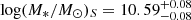 ,
,  , and
, and  /yr. As a consistency check, we calculated the SFR from the VLA/3GHz observations (following equation 12 from Kennicutt & Evans 2012). We found SFRN, VLA = 376.8 ± 6.3 M⊙/yr for North based on the single source detection reported in Smolčić et al. (2017) and SFRS, VLA ≤ 46 M⊙/yr based on the 3σ noise limit of the VLA 3GHz map for South. The results between the SFRs from the SED fitting and those based on the VLA data are thus consistent within the errors. From the CO(2–1) data analysis presented in Section 3.4, we find a molecular gas mass of
  for North and an upper limit of log(MH2/M⊙)S ≤ 10.74 for South. Therefore, we find the two galaxies to be massive SFGs, with a significant amount of molecular gas and dust. For the mass ratios, we find
  for the ratio based on the stellar masses alone and
  for the ratio based on the combination of the stellar and gas masses. This means that this system of two galaxies is a major merger (e.g. Mantha et al. 2018; Duncan et al. 2019).
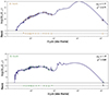 |
Fig. 6. SED fitting results for North (top) and South (bottom). The model fit is shown with the purple line, and the observations are shown with the beige (North) or green (South) dots. For South, the ALMA upper-limit observation at 1.2 μm is shown with an down-pointing arrow. |
4. Discussion
4.1. Rare major merger
Combined with ancillary data, we used ALMA CO(2–1), CO(5–4) and dust-continuum (rest-frame 520 μm) observations with an angular resolution of ≤1.3″ to reveal a heavily dust-obscured star-forming galaxy in the process of merging with another galaxy. This merger was previously identified with HST/F814W observations as a single galaxy. For the stellar mass range encompassing the galaxies in the system presented in this paper, log10(M*/M⊙) > 10.3, ≲10% of the galaxies at z ∼ 1 are in a major merger according to Duncan et al. (2019). This implies that systems like Matilda should be very rare. However, several recent works have shown the limitations of a visual merger identification. Blumenthal et al. (2020) showed, for example, that more than 50% of the mergers are missed with a visual identification of mock Sloan Digital Sky Survey (York et al. 2000) g-band images. Furthermore, most of the work on galaxy mergers, such as Tasca et al. (2014), Ventou et al. (2017), and Duncan et al. (2019), was based on the visual identification of the merger components from rest-frame optical data, which made it physically impossible to account for dusty systems such as the one presented here because dust can partially or totally obscure rest-frame optical data. Although optically faint or dark single galaxies are known at high redshift (z > 3), as shown for instance in Umehata et al. (2020), Barrufet et al. (2023), and Gómez-Guijarro et al. (2023), the situation for partly optically faint or dark systems of galaxies at lower redshift is unclear. Only a few works have reported objects that might be similar to the system we study here. One notable example is the work of Kokorev et al. 2023, who showed a massive dusty star-forming galaxy at z = 1.3844 that is not fully detected in HST/F814W observations with a potential optically dark companion. The hypothesis of an optically dark companion is supported by the tentative 2σ ALMA observations, which show a dusty structure that reaches towards a secondary star-forming region and has a similar CO(2–1) emission line profile as the region we observe in this work. The James Webb Space Telescope (JWST) might also help us to accurately assess the fraction of all galaxy mergers, including dusty systems. Recent work with JWST data has shown that more systems might belong to this specific class of galaxy mergers. For instance, Gillman et al. 2023 used JWST/NIRCam observations and identified five SMGs that could be mergers. They have NIR counterparts, but no HST optical (HST/F160W) counterparts.
4.2. Dusty galaxy merger in the context of typical star-forming galaxies
We compared the two galaxy members of the dusty z = 1.17 galaxy merger to star-forming main-sequence galaxies at that same redshift according to Speagle et al. (2014) (Figure 7). Both galaxies appear to lie above the MS (left panel of Figure 7). North exhibits a particularly high level of star formation. It appears to be more than 1 dex above the median MS and therefore falls into the regime of starburst galaxies, whereas South is nearly 0.5 dex above that median, which is consistent with MS galaxies. While the higher SFR of South can place it in the regime of starburst galaxies, its CO(5–4) to CO(2–1) line ratio seems to be rather consistent with that of MS galaxies. To our knowledge, there are no other mergers at z ∼ 1 for which multiple CO transitions are available for the each member of the merger. Information like this is available for isolated galaxies (e.g. Valentino et al. (2020), Boogaard et al. (2020), Harrington et al. (2021)), but they typically show higher CO line ratios for galaxies with SFR properties similar to those of North.
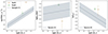 |
Fig. 7. SFR (left), depletion time (tdepl = MH2/SFR, centre), and molecular gas fraction (fgas = MH2/M*, right) of the two galaxies belonging to the dust-obscured merging system compared to the scaling relations for these properties of z = 1.17 main-sequence galaxies. North is represented by a beige marker, and South is represented by a green marker. The literature relations for the MS from Speagle et al. (2014) (left, green line) and the depletion time and gas fraction from Tacconi et al. (2018) (centre and right, beige area). |
We also evaluate dthe depletion time, that is, tdepl = MH2/SFR, of the two galaxies according to Tacconi et al. (2018) and compared them to MS z = 1.17 galaxies (central panel of Figure 7). South is consistent with MS galaxies, that is, it shows a star-forming depletion time that is consistent with the scatter of MS galaxies. We caution that the molecular gas mass derived for South is based on an upper-limit measurement of the CO(2–1) flux, and therefore, South could be forming stars even faster. North is located ∼0.5 dex below the median depletion time relation. Therefore, North is much more efficient at forming stars than South (a difference of ∼0.8 dex) and typical z = 1.17 MS galaxies by forming stars three times faster than the MS galaxies.
We determined the molecular gas fraction, that is, fgas = MH2/M*, of the two galaxies. The molecular gas fraction indicates how much molecular gas is available to form stars compared to the number of stars already formed. We again compared this quantity according to the relation for MS z = 1.17 galaxies from Tacconi et al. (2018) (right panel of Figure 7). North and South both appear to exhibit higher molecular gas fractions than MS galaxies, making them rather molecular gas-rich galaxies. Again, we caution that the molecular gas mass derived for South is based on an upper-limit measurement of the CO(2–1) flux, and the corresponding molecular gas mass fraction is therefore also an upper limit.
The two galaxies that are part of the dusty galaxy merger are both forming stars with high efficiency, and they lie accordingly above the MS. Although the two galaxies show similar gas fractions, only North is forming stars rapidly (twice as fast as MS galaxies), resulting in a starburst-like SFR. It is unclear why only one galaxy appears to have the high sSFR of a starburst although both exhibit consistently high gas fractions. Possible scenarios involve the orientation and relative rotation directions, as shown in simulations (e.g. Di Matteo et al. 2007; Cox et al. 2008), an AGN boosting the SFR of North (e.g. Hopkins et al. 2008; Cicone et al. 2014), or simply a difference in the baryonic properties of the two galaxies prior to the merger.
4.3. Effect of the merger on the properties of galaxies
Both galaxies in this dusty merger show relatively high levels of star formation and star formation efficiency (see Figure 7, left and middle panels). Moreover, as mentioned in Section 3.4, a lower αCO value would result in lower molecular gas masses, which would strengthen the star formation efficiencies even more. Therefore, the star-forming properties of the two galaxies appear to be consistent with a scenario in which mergers tend to enhance star formation (e.g. Kim et al. 2009; Saitoh et al. 2009; Kaviraj et al. 2015; Tacchella et al. 2016; Pearson et al. 2019). However, the merging process could impact each galaxy differently. North has a significantly higher SFR (a difference of a factor of 10), a slightly higher dust mass, and likely a higher CO(5–4) to CO(2–1) ratio. The origin of this different impact could also be due to a difference in the evolution and composition of the galaxies prior to their collision. Similarly, only North exhibits bright dust emission, making it almost entirely invisible in the rest-frame optical wavelengths (see Figure 3). This large amount of dust emission, high SFR, and high dust and stellar masses might indicate a merger-driven SMG phase (e.g. Blain et al. 2002; Tacconi et al. 2008; McAlpine et al. 2019). However, it remains unclear whether the high brightness of the dust emission is intrinsic to the galaxy or due to the high level of star formation, which results in a strong heating of the dust.
The multiple-transition CO observations and their spectral resolution indicate that complex dynamics are at play in the merger (3.2). The slight offset in the negative and positive velocity peaks in CO(2–1) and CO(5–4) at the location of North (see right column of Figure 5) suggest signs of rotation in the galaxy, with the northern part moving away from us (negative velocities) and the southern part approaching (positive velocities). South only seems to be traced by the negative velocity peak in both CO(2–1) and CO(5–4). This suggests that South is approaching us. The lack of observed rotation as seen for North might indicate that South is seen face-on, which is consistent with what we observe in the HST/F814W image (see Figure 3).
5. Summary and conclusions
Using ALMA archival data, we have uncovered a dusty galaxy major merger at z ∼ 1, and we studied the baryonic properties of the individual galaxies that are part of this system. We list our main findings below.
-
The ALMA CO(2–1), CO(5–4) and dust-continuum observations reveals a dust-obscured galaxy at z = 1.17.
-
These observations, complemented by other Subaru, Ultravista, HST, and Spitzer observations, show that the dust-obscured galaxy is merging with another galaxy that was previously classified (Weaver et al. 2022) as a single star-forming galaxy at z = 1.17.
-
The two galaxies have a high SFR and a short gas depletion time with respect to literature relations for main-sequence z = 1.17 galaxies. This is consistent with a picture in which mergers enhance star formation.
With the work presented in this paper, we highlight the necessity for multi-wavelength observations with observatories such as ALMA or JWST to properly assess the fraction of galaxy mergers in our Universe. With their longer wavelengths, ALMA and JWST can observe systems that are otherwise obscured at rest-frame optical and NIR wavelengths. For instance, Jones et al. (2024) used the high spatial and spectral resolution of JWST to reveal four galaxies that initially appeared as one single massive starburst galaxy (Riechers et al. 2013). This clearly showcased the importance of high resolution to properly account for mergers. The ALMA archive represents the ideal database to find a hidden fraction of galaxy mergers because the (sub)millimeter wavelengths can observe the dust, and the large number of data increases the probability of finding more systems such as the system we presented in this paper. JWST, specifically, the MIRI instrument, offers a high sensitivity, a large field of view compared to ALMA (73.5″ × 112.6″), and a high spatial resolution. This is ideal for separating faint dusty systems. Due to the different wavelength range probed by ALMA and JWST/MIRI, the observations would trace different types of dust (cold and hot). Therefore, using the two telescopes in synergy would enable a more complete view of the dust in this class of dusty galaxy mergers. With the available angular resolution of the archival ALMA data and the assumptions we presented here, we were able to use dust-continuum and multiple CO transitions observations to study the gas and dust content of the two galaxies involved in this merger, which was serendipituously discovered. Observations with a higher resolution would enable a better informed assumption and even a more detailed study of the gas within the galaxies, that is, the ISM, and its structure and dynamics. The gravitational forces between galaxies in a merger can significantly disrupt their structures. Tidal forces arise that distort the galaxy shapes and disrupt their gas, dust, and stars, leaving tidal streams as imprints of the merger process (e.g. Stewart et al. 2011; Guo et al. 2016; Ginolfi et al. 2020). The merger presented in this paper would be an ideal laboratory for studying these tidal streams because its dust content is large and because the two galaxies are close (≤10 kpc apart).
The nickname comes from the name of the cat living at the base camp of the Atacama Pathfinder Experiment telescope, where the work presented in this paper started.
Acknowledgments
We thank the anonymous referee for their careful and constructive report that greatly improved the clarity and quality of this paper. This paper makes use of the following ALMA data: ADS/JAO.ALMA#2015.1.00260.S and ADS/JAO.ALMA#016.1.00171.S. ALMA is a partnership of ESO (representing its member states), NSF (USA) and NINS (Japan), together with NRC (Canada), MOST and ASIAA (Taiwan), and KASI (Republic of Korea), in cooperation with the Republic of Chile. The Joint ALMA Observatory is operated by ESO, AUI/NRAO and NAOJ. This research has made use of the NASA/IPAC Infrared Science Archive, which is funded by the National Aeronautics and Space Administration and operated by the California Institute of Technology. FG acknowledges the support from grant PRIN MIUR 2017-20173ML3WW_001. “Opening the ALMA window on the cosmic evolution of gas, stars, and supermassive black holes”. We thank Nicolas Bouché and Mark Swinbank for useful discussions and feedback.
References
- Aihara, H., AlSayyad, Y., Ando, M., et al. 2019, PASJ, 71, 114 [Google Scholar]
- Barrufet, L., Oesch, P. A., Weibel, A., et al. 2023, MNRAS, 522, 449 [NASA ADS] [CrossRef] [Google Scholar]
- Battisti, A. J., Cunha, E. D., Shivaei, I., & Calzetti, D., 2020, ApJ, 888, 108 [NASA ADS] [CrossRef] [Google Scholar]
- Behiri, M., Talia, M., Cimatti, A., et al. 2023, ApJ, 957, 63 [NASA ADS] [CrossRef] [Google Scholar]
- Blain, A. W., Smail, I., Ivison, R. J., Kneib, J. P., & Frayer, D. T. 2002, Phys. Rep., 369, 111 [Google Scholar]
- Blumenthal, K. A., Moreno, J., Barnes, J. E., et al. 2020, MNRAS, 492, 2075 [CrossRef] [Google Scholar]
- Bolatto, A. D., Wolfire, M., & Leroy, A. K. 2013, ARA&A, 51, 207 [CrossRef] [Google Scholar]
- Boogaard, L. A., van der Werf, P., Weiss, A., et al. 2020, ApJ, 902, 109 [NASA ADS] [CrossRef] [Google Scholar]
- Bothwell, M. S., Smail, I., Chapman, S. C., et al. 2013, MNRAS, 429, 3047 [Google Scholar]
- Bradley, L. 2023, https://doi.org/10.5281/zenodo.7946442 [Google Scholar]
- Byrne-Mamahit, S., Hani, M. H., Ellison, S. L., Quai, S., & Patton, D. R. 2023, MNRAS, 519, 4966 [NASA ADS] [CrossRef] [Google Scholar]
- Carilli, C. L., & Walter, F. 2013, ARA&A, 51, 105 [NASA ADS] [CrossRef] [Google Scholar]
- CASA Team (Bean, B., et al.) 2022, PASP, 134 [Google Scholar]
- Casteels, K. R. V., Conselice, C. J., Bamford, S. P., et al. 2014, MNRAS, 445, 1157 [NASA ADS] [CrossRef] [Google Scholar]
- Chabrier, G. 2003, PASP, 115, 763 [Google Scholar]
- Cicone, C., Maiolino, R., Sturm, E., et al. 2014, A&A, 562, A21 [NASA ADS] [CrossRef] [EDP Sciences] [Google Scholar]
- Conselice, C. J., Mundy, C. J., Ferreira, L., & Duncan, K. 2022, ApJ, 940, 168 [CrossRef] [Google Scholar]
- Cortes, P., Vlahakis, C., Hales, A., et al. 2023, https://doi.org/10.5281/zenodo.7822943 [Google Scholar]
- Cox, T. J., Jonsson, P., Somerville, R. S., Primack, J. R., & Dekel, A. 2008, MNRAS, 384, 386 [NASA ADS] [CrossRef] [Google Scholar]
- da Cunha, E., Walter, F., Smail, I. R., et al. 2015, ApJ, 806, 110 [Google Scholar]
- Di Matteo, P., Combes, F., Melchior, A. L., & Semelin, B. 2007, A&A, 468, 61 [NASA ADS] [CrossRef] [EDP Sciences] [Google Scholar]
- Duncan, K., Conselice, C. J., Mundy, C., et al. 2019, ApJ, 876, 110 [NASA ADS] [CrossRef] [Google Scholar]
- Ellison, S. L., Wilkinson, S., Woo, J., et al. 2022, MNRAS, 517, L92 [NASA ADS] [CrossRef] [Google Scholar]
- Endsley, R., Stark, D. P., Charlot, S., et al. 2021, MNRAS, 502, 6044 [NASA ADS] [CrossRef] [Google Scholar]
- Enia, A., Talia, M., Pozzi, F., et al. 2022, ApJ, 927, 204 [NASA ADS] [CrossRef] [Google Scholar]
- Euclid Collaboration (Moneti, A., et al.) 2022, A&A, 658, A126 [NASA ADS] [CrossRef] [EDP Sciences] [Google Scholar]
- Gaia Collaboration (Brown, A. G. A., et al.) 2018, A&A, 616, A1 [NASA ADS] [CrossRef] [EDP Sciences] [Google Scholar]
- Gentile, F., Talia, M., Behiri, M., et al. 2023, ArXiv e-prints [arXiv:2312.05305] [Google Scholar]
- Gillman, S., Gullberg, B., Brammer, G., et al. 2023, A&A, 676, A26 [NASA ADS] [CrossRef] [EDP Sciences] [Google Scholar]
- Ginolfi, M., Jones, G. C., Béthermin, M., et al. 2020, A&A, 643, A7 [NASA ADS] [CrossRef] [EDP Sciences] [Google Scholar]
- Gómez-Guijarro, C., Magnelli, B., Elbaz, D., et al. 2023, A&A, 677, A34 [NASA ADS] [CrossRef] [EDP Sciences] [Google Scholar]
- Guo, R., Hao, C.-N., Xia, X. Y., Mao, S., & Shi, Y. 2016, ApJ, 826, 30 [NASA ADS] [CrossRef] [Google Scholar]
- Harrington, K. C., Weiss, A., Yun, M. S., et al. 2021, ApJ, 908, 95 [NASA ADS] [CrossRef] [Google Scholar]
- Hatziminaoglou, E., Zwaan, M., Andreani, P., et al. 2015, The Messenger, 162, 24 [NASA ADS] [Google Scholar]
- Hopkins, P. F., Hernquist, L., Cox, T. J., & Kereš, D. 2008, ApJS, 175, 356 [Google Scholar]
- Jin, S., Daddi, E., Liu, D., et al. 2018, ApJ, 864, 56 [Google Scholar]
- Jones, G. C., Ubler, H., Perna, M., et al. 2024, A&A, 682, A122 [NASA ADS] [CrossRef] [EDP Sciences] [Google Scholar]
- Kaviraj, S., Cohen, S., Windhorst, R. A., et al. 2013, MNRAS, 429, L40 [NASA ADS] [Google Scholar]
- Kaviraj, S., Devriendt, J., Dubois, Y., et al. 2015, MNRAS, 452, 2845 [Google Scholar]
- Kennicutt, R. C., & Evans, N. J. 2012, ARA&A, 50, 531 [NASA ADS] [CrossRef] [Google Scholar]
- Kim, J.-H., Wise, J. H., & Abel, T. 2009, ApJ, 694, L123 [NASA ADS] [CrossRef] [Google Scholar]
- Koekemoer, A. M., Aussel, H., Calzetti, D., et al. 2007, ApJS, 172, 196 [Google Scholar]
- Kokorev, V., Jin, S., Gómez-Guijarro, C., et al. 2023, A&A, 677, A172 [NASA ADS] [CrossRef] [EDP Sciences] [Google Scholar]
- Labbé, I., Bouwens, R., Illingworth, G. D., & Franx, M. 2006, ApJ, 649, L67 [CrossRef] [Google Scholar]
- Laigle, C., McCracken, H. J., Ilbert, O., et al. 2016, ApJS, 224, 24 [Google Scholar]
- Lotz, J. M., Jonsson, P., Cox, T. J., & Primack, J. R. 2008, MNRAS, 391, 1137 [Google Scholar]
- Madau, P., & Dickinson, M. 2014, ARA&A, 52, 415 [Google Scholar]
- Mantha, K., McIntosh, D. H., Conselice, C., et al. 2018, in American Astronomical Society Meeting Abstracts #231, 258.01 [Google Scholar]
- Martin, G., Kaviraj, S., Devriendt, J. E. G., Dubois, Y., & Pichon, C. 2018, MNRAS, 480, 2266 [Google Scholar]
- Massey, R., Stoughton, C., Leauthaud, A., et al. 2010, MNRAS, 401, 371 [NASA ADS] [CrossRef] [Google Scholar]
- McAlpine, S., Smail, I., Bower, R. G., et al. 2019, MNRAS, 488, 2440 [NASA ADS] [CrossRef] [Google Scholar]
- McCracken, H. J., Milvang-Jensen, B., Dunlop, J., et al. 2012, A&A, 544, A156 [NASA ADS] [CrossRef] [EDP Sciences] [Google Scholar]
- Mundy, C. J., Conselice, C. J., Duncan, K. J., et al. 2017, MNRAS, 470, 3507 [Google Scholar]
- Pearson, W. J., Wang, L., Alpaslan, M., et al. 2019, A&A, 631, A51 [NASA ADS] [CrossRef] [EDP Sciences] [Google Scholar]
- Planck Collaboration VI. 2020, A&A, 641, A6 [NASA ADS] [CrossRef] [EDP Sciences] [Google Scholar]
- Ren, J., Li, N., Liu, F. S., et al. 2023, ArXiv e-prints [arXiv:2309.16531] [Google Scholar]
- Riechers, D. A., Bradford, C. M., Clements, D. L., et al. 2013, Nature, 496, 329 [Google Scholar]
- Romano, M., Cassata, P., Morselli, L., et al. 2021, A&A, 653, A111 [NASA ADS] [CrossRef] [EDP Sciences] [Google Scholar]
- Saitoh, T. R., Daisaka, H., Kokubo, E., et al. 2009, PASJ, 61, 481 [NASA ADS] [Google Scholar]
- Scoville, N., Aussel, H., Brusa, M., et al. 2007, ApJS, 172, 1 [Google Scholar]
- Smail, I., Dudzevičiūtė, U., Gurwell, M., et al. 2023, ApJ, 958, 36 [NASA ADS] [CrossRef] [Google Scholar]
- Smolčić, V., Novak, M., Bondi, M., et al. 2017, A&A, 602, A1 [Google Scholar]
- Speagle, J. S., Steinhardt, C. L., Capak, P. L., & Silverman, J. D. 2014, ApJS, 214, 15 [Google Scholar]
- Spilker, J. S., Marrone, D. P., Aguirre, J. E., et al. 2014, ApJ, 785, 149 [NASA ADS] [CrossRef] [Google Scholar]
- Stewart, K. R., Kaufmann, T., Bullock, J. S., et al. 2011, ApJ, 738, 39 [NASA ADS] [CrossRef] [Google Scholar]
- Tacchella, S., Dekel, A., Carollo, C. M., et al. 2016, MNRAS, 457, 2790 [Google Scholar]
- Tacconi, L. J., Genzel, R., Smail, I., et al. 2008, ApJ, 680, 246 [Google Scholar]
- Tacconi, L. J., Genzel, R., Saintonge, A., et al. 2018, ApJ, 853, 179 [Google Scholar]
- Talia, M., Cimatti, A., Giulietti, M., et al. 2021, ApJ, 909, 23 [NASA ADS] [CrossRef] [Google Scholar]
- Tasca, L. A. M., Le Fèvre, O., López-Sanjuan, C., et al. 2014, A&A, 565, A10 [NASA ADS] [CrossRef] [EDP Sciences] [Google Scholar]
- Umehata, H., Smail, I., Swinbank, A. M., et al. 2020, A&A, 640, L8 [NASA ADS] [CrossRef] [EDP Sciences] [Google Scholar]
- Valentino, F., Daddi, E., Puglisi, A., et al. 2020, A&A, 641, A155 [NASA ADS] [CrossRef] [EDP Sciences] [Google Scholar]
- Ventou, E., Contini, T., Bouché, N., et al. 2017, A&A, 608, A9 [NASA ADS] [CrossRef] [EDP Sciences] [Google Scholar]
- Ventou, E., Contini, T., Bouche, N., et al. 2019, VizieR Online Data Catalog, J/A+A/631/A87 [Google Scholar]
- Weaver, J. R., Kauffmann, O. B., Ilbert, O., et al. 2022, ApJS, 258, 11 [NASA ADS] [CrossRef] [Google Scholar]
- Whitler, L., Stark, D. P., Endsley, R., et al. 2023, MNRAS, 519, 5859 [NASA ADS] [CrossRef] [Google Scholar]
- York, D. G., Adelman, J., Anderson, J. E. Jr, et al. 2000, AJ, 120, 1579 [Google Scholar]
- Zavala, J. A., Casey, C. M., Manning, S. M., et al. 2021, ApJ, 909, 165 [CrossRef] [Google Scholar]
Appendix A: Example of the PhoEBO code
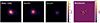 |
Fig. A.1. The Spitzer/IRAC Channel 2 maps resulting from the deblending performed by PhoEBO. From left to right: Input map to deblend, output deblended map of North, output deblended map of South, and residuals of the modelling (i.e., input map subtracted from the sum of the two outputs). |
All Tables
All Figures
|
Fig. 1. CO(2–1) (left) and CO(5–4) (right) emissions of the entire system in mJy per 75 km/s as a function of the velocity, where the centre velocity is determined from the redshift z = 1.17. The channels used to create the intensity maps are highlighted with the grey shaded area. |
| In the text | |
|
Fig. 2. Intensity maps (7″ × 7″) of the CO(2–1) emission (left) with [3, 4, 5, 6] σCO(2 − 1) contours, the CO(5–4) emission (middle) with [3, 4, 5, 6] σCO(5 − 4) contours, and the dust-continuum image (right) with [3, 5, 7, 9, 11] σdust contours. |
| In the text | |
|
Fig. 3. HST F814W image from Koekemoer et al. (2007), with ALMA CO(2–1) contours in blue at [3, 4, 5, 6] σCO(2 − 1) and ALMA dust-continuum in beige at [3, 5, 7, 9, 11] σdust. The beams are shown in the lower left, with sizes of 1.3″ and 0.8″ for the CO(2–1) and dust-continuum emissions, respectively. A scale is shown at the bottom right to represent the physical scales at the redshift of the system, i.e., z = 1.17. |
| In the text | |
|
Fig. 4. ALMA CO(2–1) emission contours (in blue) and HST/F814W emission contours (in white) overlaid on Ultravista Ks band (left), IRAC channel 2 (middle), and VLA 10 cm (right) observations. These images are postage stamps of 5″ × 5″. |
| In the text | |
|
Fig. 5. Contours of the CO(2–1) (top row) and CO(5–4) (bottom row) intensity maps when integrating around the negative velocity peak (left column, solid lines) or the right peak (middle column, dash-dotted lines) of the emissions. The right column shows the two peaks overlaid. The negative and positive velocity peaks correspond to −575 km/s, −50 km/s, and −50 km/s to −475 km/s, respectively, for the CO(2–1) and CO(5–4) emissions. The contours start at 3σ and increase with an indent of 1σ. The background image in the top row (bottom row) is the CO(2–1) (CO(5–4)) emission when integrating the entire peak, as shown in the left (right) panel of Figure 2. The inset shows the spectrum, and the channels we used in the imaging are highlighted with the grey shaded area. |
| In the text | |
|
Fig. 6. SED fitting results for North (top) and South (bottom). The model fit is shown with the purple line, and the observations are shown with the beige (North) or green (South) dots. For South, the ALMA upper-limit observation at 1.2 μm is shown with an down-pointing arrow. |
| In the text | |
|
Fig. 7. SFR (left), depletion time (tdepl = MH2/SFR, centre), and molecular gas fraction (fgas = MH2/M*, right) of the two galaxies belonging to the dust-obscured merging system compared to the scaling relations for these properties of z = 1.17 main-sequence galaxies. North is represented by a beige marker, and South is represented by a green marker. The literature relations for the MS from Speagle et al. (2014) (left, green line) and the depletion time and gas fraction from Tacconi et al. (2018) (centre and right, beige area). |
| In the text | |
|
Fig. A.1. The Spitzer/IRAC Channel 2 maps resulting from the deblending performed by PhoEBO. From left to right: Input map to deblend, output deblended map of North, output deblended map of South, and residuals of the modelling (i.e., input map subtracted from the sum of the two outputs). |
| In the text | |
Current usage metrics show cumulative count of Article Views (full-text article views including HTML views, PDF and ePub downloads, according to the available data) and Abstracts Views on Vision4Press platform.
Data correspond to usage on the plateform after 2015. The current usage metrics is available 48-96 hours after online publication and is updated daily on week days.
Initial download of the metrics may take a while.