| Issue |
A&A
Volume 689, September 2024
|
|
|---|---|---|
| Article Number | A51 | |
| Number of page(s) | 13 | |
| Section | Numerical methods and codes | |
| DOI | https://doi.org/10.1051/0004-6361/202449173 | |
| Published online | 02 September 2024 | |
Bayesian inference of multi-messenger astrophysical data: Joint and coherent inference of gravitational waves and kilonovae
1
Theoretisch-Physikalisches Institut, Friedrich-Schiller-Universität Jena,
Fröbelstieg 1,
07743
Jena,
Germany
e-mail: This email address is being protected from spambots. You need JavaScript enabled to view it.
2
Scuola Internazionale Superiore di Studi Avanzati (SISSA),
Via Bonomea 265,
34136
Trieste,
Italy
3
Istituto Nazionale di Fisica Nucleare (INFN),
Sezione di Trieste, Via Valerio 2,
34127
Trieste,
Italy
4
Institute for Gravitation & the Cosmos, The Pennsylvania State University,
University Park,
PA
16802,
USA
5
Department of Physics, University of California,
Berkeley,
CA
94720,
USA
6
Niels Bohr International Academy, Niels Bohr Institute,
Blegdamsvej 17,
2100
Copenhagen,
Denmark
7
Dipartimento di Fisica, Università di Trento,
Via Sommarive 14,
38123
Trento,
Italy
8
INFN-TIFPA, Trento Institute for Fundamental Physics and Applications,
Via Sommarive 14,
38123
Trento,
Italy
9
Department of Physics, The Pennsylvania State University,
University Park,
PA
16802,
USA
10
Department of Astronomy & Astrophysics, The Pennsylvania State University,
University Park,
PA
16802,
USA
Received:
8
January
2024
Accepted:
16
May
2024
Abstract
Context. Multi-messenger observations of binary neutron star mergers can provide information on the neutron star’s equation of state (EOS) above the nuclear saturation density by directly constraining the mass-radius diagram.
Aims. We present a Bayesian framework for joint and coherent analyses of multi-messenger binary neutron star signals. As a first application, we analyze the gravitational-wave GW170817 and the kilonova (kN) AT2017gfo data. These results are then combined with the most recent X-ray pulsar analyses of PSR J0030+0451 and PSR J0740+6620 to obtain new EOS constraints.
Methods. We extend the bajes infrastructure with a joint likelihood for multiple datasets, support for various semi-analytical kN models, and numerical-relativity (NR)-informed relations for the mass ejecta, as well as a technique to include and marginalize over modeling uncertainties. The analysis of GW170817 used the TEOBResumS effective-one-body waveform template to model the gravitational-wave signal. The analysis of AT2017gfo used a baseline multicomponent spherically symmetric model for the kN light curves. Various constraints on the mass-radius diagram and neutron star properties were then obtained by resampling over a set of ten million parameterized EOSs, which was built under minimal assumptions (general relativity and causality).
Results. We find that a joint and coherent approach improves the inference of the extrinsic parameters (distance) and, among the intrinsic parameters, the mass ratio. The inclusion of NR-informed relations marks a strong improvement over the case in which an agnostic prior is used on the intrinsic parameters. Comparing Bayes factors, we find that the two observations are better explained by the common source hypothesis only by assuming NR-informed relations. These relations break some of the degeneracies in the employed kN models. The EOS inference folding-in PSR J0952-0607 minimum-maximum mass, PSR J0030+0451 and PSR J0740+6620 data constrains, among other quantities, the neutron star radius to R1.4TOV = 12.30− 0.56+ 0.81 km(R1.4TOV = 13.20− 0.90+ 0.91 km) and the maximum mass to MmaxTOV = 2.28− 0.17+ 0.25M⊙(MmaxTOV = 2.32− 0.19+ 0.30M⊙), where the ST+PDT (PDT-U) analysis of Vinciguerra et al. (2024, ApJ, 961, 62) for PSR J0030+0451 was employed. Hence, the systematics on the PSR J0030+0451 data reduction currently dominate the mass-radius diagram constraints.
Conclusions. We conclude that bajes delivers robust analyses in line with other state-of-the-art results in the literature. Strong EOS constraints are provided by pulsars observations, albeit with large systematics in some cases. Current gravitational-wave constraints are compatible with pulsar constraints and can further improve the latter.
Key words: gravitational waves / methods: data analysis / stars: neutron / pulsars: general
Alfred P. Sloan Fellow.
© The Authors 2024
 Open Access article, published by EDP Sciences, under the terms of the Creative Commons Attribution License (https://creativecommons.org/licenses/by/4.0), which permits unrestricted use, distribution, and reproduction in any medium, provided the original work is properly cited.
This article is published in open access under the Subscribe to Open model. This email address is being protected from spambots. You need JavaScript enabled to view it. to support open access publication.
1 Introduction
The observation of a gravitational wave (GW) signal GW170817 from a binary neutron star (NS) merger and its electromagnetic counterparts from the merger aftermath opened up new prospects of constraining the nature of NS matter (Acernese et al. 2015; LIGO Scientific Collaboration 2015; LIGO Scientific Collaboration and Virgo Collaboration 2017c,b, 2019b). The GWs from the late-inspiral-to-merger frequencies carry the imprint of short-range tidal interactions between the two NSs (Damour & Deruelle 1986; Damour & Nagar 2010). The measurement of tidal polarizability parameters, in particular the reduced tidal parameter,  , appearing in the leading-order term of the GW phase (Damour et al. 2012; Favata 2014), constrains the nuclear equation of state (EOS) (LIGO Scientific Collaboration and Virgo Collaboration 2018; De et al. 2018; LIGO Scientific Collaboration and Virgo Collaboration 2020). For GW170817, various analyses indicate posterior distributions peaking in the interval
  , which can be mapped onto an NS radius1 constraint of
  km with 90% credibility (Gamba et al. 2021b).
Electromagnetic counterparts can complement such constraints by delivering information on the merger remnant. For example, the high-energy emission from a jet-like source of GRB170817 (LIGO Scientific Collaboration and Virgo Collaboration 2017b; Savchenko et al. 2017) is associated with the presence of a remnant black hole and can thus constrain the maximum NS mass (Margalit & Metzger 2017; Shibata et al. 2017; see also Margalit et al. 2022 for a revision of the first calculation). The intepretation of the kilonova (kN) AT2017gfo (Coulter et al. 2017; Chornock et al. 2017; Nicholl et al. 2017; Cowperthwaite et al. 2017; Pian et al. 2017; Smartt et al. 2017; Tanvir et al. 2017; Tanaka et al. 2017; Valenti et al. 2017) requires different mass ejecta components (LIGO Scientific Collaboration and Virgo Collaboration 2017a; Villar et al. 2017; Perego et al. 2017b; Breschi et al. 2021b), and thus excludes prompt black hole formation (Margalit & Metzger 2017; Bauswein et al. 2017). Further, the necessity of including a massive disk wind to interpret the light curves implies a lower limit (as opposed to the GW upper limit) on the reduced tidal parameter (Radice et al. 2018c,b).
Rigorous analysis of multi-messenger astrophysics (MMA) data requires a Bayesian approach. Bayesian inference of GW170817 and related counterparts with application to the NS EOS has been performed by various authors (Radice & Dai 2019; Coughlin et al. 2019; Capano et al. 2020; Coughlin & Dietrich 2019; Jiang et al. 2020; Essick et al. 2020; Dietrich et al. 2020; Al-Mamun et al. 2021; Nicholl et al. 2021; Breschi et al. 2021b; Raaijmakers et al. 2021a; Ayriyan et al. 2021; Huth et al. 2022; Pang et al. 2022; Brandes et al. 2023; Zhu et al. 2023; Fan et al. 2024). These analyses provide bounds or posterior distributions on fiducial NS masses, radii, quadrupolar tidal polarizability parameters, pressure (or energy density), sound speed at fiducial points, or even nuclear parameters (given an EOS parameterization). Some results about the NS radius are collected in Fig. 12 of Breschi et al. (2021b), indicating a substantial agreement among various analyses, with  km and 90% credible intervals at the kilometer level, depending on the specific assumptions. In several cases, these analyses incorporate an assumption about the EOS (Jiang et al. 2020; Greif et al. 2020; Huang et al. 2023; Fan et al. 2024) including available experimental nuclear data (Danielewicz et al. 2002; Hebeler et al. 2013; Le Fèvre et al. 2016; Russotto et al. 2016). Despite the potential for MMA observations of NS mergers, data from GW170817 and its counterparts alone do not yet significantly constrain the nuclear physics of dense NS matter (Al-Mamun et al. 2021; Greif et al. 2020). The lower bound of the maximum NS mass,
  (“minimum-maximum mass”), provided by pulsar observations (Demorest et al. 2010; Miller et al. 2019; Romani et al. 2022; Godzieba et al. 2021), gives the strongest constraint on nuclear matter. Those data rule out a large number of EOS models, including some containing hyperons or decon-fined quark matter (Hebeler et al. 2013) (though the latter are still viable; see e.g., Annala et al. 2020). The most massive NS identified so far is PSR J0952-0607, a millisecond pulsar in a binary system, with MJ0740+6620 = 2.35 ± 0.17 M⊙ (Romani et al. 2022). Recent X-ray observations of isolated pulsars have been performed by NICER and XMM-Newton (Miller, 2021; Riley et al. 2019, 2021). These observations targeted PSR J0030+0451 (Miller et al. 2019; Riley et al. 2021; Raaijmakers et al. 2019) and PSR J0740+6620 (Miller et al. 2021). The former NS has a best radius and mass estimates of
  km and
  (68% credibility) (Miller et al. 2019) (see also Riley et al. 2019). The latter NS has the second-heaviest reliably determined mass to date, MJ0740+6620 = 2.08 ± 0.07M⊙, with a radius of
  km (68% credibility) (Miller et al. 2021). Overall, these data constrain the mass and radius of the NS at a level of ≲5%. Several MMA analyses have combined BNS mergers with pulsar data; that is, they have used data from multiple sources to improve astrophysical EOS constraints (Jiang et al. 2020; Essick et al. 2020; Dietrich et al. 2020; Al-Mamun et al. 2021; Nicholl et al. 2021; Breschi et al. 2021b; Raaijmakers et al. 2021a; Ayriyan et al. 2021; Brandes et al. 2023; Fan et al. 2024). Recently, Vinciguerra et al. (2024) reanalyzed PSR J0030+0451 with an improved pipeline, finding updated measurements of both the mass and radius of the pulsar depending on the hotspot model employed:
  (ST+PDT) or
  (PDT-U).
Methodologically, MMA analyses share several common features. We comment on three such common elements, which are later incorporated into our work. (i) The use of phenomeno-logical relations from numerical-relativity (NR) simulations, incorporating remnant constraints into GW analysis. Accurate simulation results are, for example, available to build equal-mass prompt collapse models (Hotokezaka et al. 2011; Bauswein et al. 2013a; Agathos et al. 2020; Kashyap et al. 2022; Perego et al. 2022). Simple models describing kinematic quantities of dynamical ejecta (Dietrich & Ujevic 2017; Radice et al. 2018b; Krüger & Foucart 2020; Nedora et al. 2022) and remnant disk masses (Radice et al. 2018b; Krüger & Foucart 2020; Nedora et al. 2022) in terms of the binary properties are also available. However, such relationships are subject to significant systemat-ics, depending on the physics input of the simulations (Nedora et al. 2022). (ii) The assumption of an EOS catalog in order to map the posteriors of the inferred parameters into another set of parameters. The typical sample size of this catalog ranges from a few tens of EOS curves to a few thousand. These EOS sets may be constructed from model-agnostic piecewise polytropic representations (Jiang et al. 2020; Raaijmakers et al. 2021a) or by assuming nuclear theories such as Chiral effective theory and perturbative quantum chromodynamics in their regime of validity (Essick et al. 2020; Fan et al. 2024). This implies different prior assumptions between different analyses, and makes a direct comparison of the results problematic. However, it should be noted that the vast majority of the EOS sets employed include constraints coming from massive pulsars (Antoniadis et al. 2013; Cromartie et al. 2019), sharing part of their prior information (additional details are provided below). (iii) The MMA analyses are often performed independently for each dataset, combining in post-processing the posterior distributions for the relevant parameters. While this approach is justified for data coming from independent sources, the analysis of different data from a single source may benefit from joint coherent analyses, especially in the case of large correlations between parameters describing the different dataset and in the presence of modeling systematics. The single-source-multiple-data scenario can be rigorously handled within the Bayesian framework by joining the single-messenger likelihoods and performing a combined sampling of the full posterior probability distribution (Biscoveanu et al. 2020; Pang et al. 2022); we refer to these analyses as “joint and coherent.”
In this work, we present anew framework for joint and coherent MMA Bayesian analyses. We apply our framework to the case of GW170817 and AT2017gfo and provide updated constraints on the NS EOS. The structure and summary of the paper is as follows. Section 2 describes the methods employed in our analysis, and presents the extension of the bajes pipeline (Breschi et al. 2021b) to MMA data. Section 3 describes the results of applying bajes-MMA to GW170817 and AT2017gfo data. We employ a state-of-the-art effective-one-body (EOB) template and a spherically symmetric multicomponent semi-analytical kN model. We compare single-messenger analyses to joint and coherent analyses using either an agnostic prior on intrinsic parameters or an NR-informed prior on intrinsic parameters. Section 4 discusses EOS constraints from our new analyses. We use a set of ~10 million parameterized EOSs built under minimal assumptions; namely, assuming general relativity, causality, and a minimum-maximum mass of 2.09 M⊙ (Romani et al. 2022). We combine GW170817+At2017gfo data with independent pulsar data and include, for the first time, the recent reanalysis of Vinciguerra et al. (2024). Conclusions and an appendix on new fitting formulas close the paper.
2 Methods
Our analyses are based on Bayesian probability, which delivers information on the source parameters in terms of their posterior probability distributions, an accurate characterization of the correlations among parameters, and the possibility of ranking different hypotheses to explain the data (e.g. Jeffreys 1939). Given the observed data, d, and a set of parameters, θ, which characterize a model of the data (hypothesis H), the information on the parameters is encoded in the posterior distribution, p(θ|d, H). Using Bayes theorem, p(θ|d, H) can be computed as the product of the likelihood function, p(d|θ, H), and the prior distribution of the model parameters, p(θ|H). The evidence, p(d|H), is instead employed in the context of model selection in order to discriminate between different models. Given two different hypotheses, say HA and HB, the Bayes factor (BF),
 (1)
(1)
encodes the support of the data in favoring hypothesis A over hypothesis B (within the assumption of a uniform prior on HA,B)2.
For multi-messenger astrophysics data, the high-dimensional parameters’ posterior distribution can have nontrivial correlations and multi-modalities. Numerical stochastic methods are essential tools for performing parameter estimation (PE). We employed the bajes pipeline (Breschi et al. 2021b) together with the nested sampling algorithm (e.g. Skilling 2006; Feroz et al. 2009), implemented in the DYNESTY nested sampler (Speagle 2020). All the PE runs presented here were performed with 5000 live points and using bajes parallel capabilities. In the following, we describe the data, the likelihood functions, the models, and the prior utilized in the analyses.
2.1 Gravitational wave inference
The time series recorded by the ground-based interferometers LIGO and Virgo can be modeled as the sum of a noise contribution, n(t), and a GW transient, h(t); that is, d(t) = h(t) + n(t). The signal observed by the interferometers was computed from the GW polarizations, h+,×, as
 (2)
(2)
where F+,× are the antenna pattern functions of the employed detector (see, e.g. Anderson et al. 2001), which are functions of the source location, {α,δ}, and the polarization angle, ψ. We analyzed the GW data segment, d(t), from the Gravitational-Wave Open Science Center (GWOSC) centered around GPS time 1187008857 with a duration of T = 128 s and sampling rate of 4096 Hz (LIGO Scientific Collaboration and Virgo Collaboration 2017c, 2019a).
We analyzed the GW signal, h(t), assuming a quasi-circular binary neutron star (BNS) merger and employing the EOB model TEOBResumS (Bernuzzi et al. 2015; Nagar et al. 2018, 2020; Akcay et al. 2019; Gamba et al. 2021a) with tidal and non-precessing spin interactions. We included the dominant quadrupolar (2, 2) mode of radiation in the waveform construction, and for efficiency used the post-adiabatic method (Nagar & Rettegno 2019) for the EOB dynamics and the stationary-phase approximation for frequency domain waveforms (Gamba et al. 2021a). We stress that this EOB model is faithful to NR within its error bands, and that systematic errors due to modeling choices are sub-dominant with respect to statistical uncertainties in the GW analysis (LIGO Scientific Collaboration and Virgo Collaboration 2019b; Gamba et al. 2021b).
The GW template, h(t; θgw), was parameterized by 11 degrees of freedom,
 (3)
(3)
where m1,2 are the component masses, are the components of dimensionless spins aligned with the orbital angular momentum, Λ1,2 are the dimensionless quadrupolar tidal polarizabilities, is the luminosity distance, ιgw is the inclination angle between the line of sight and the total angular momentum of the system, and tmrggw and ϕmrg are, respectively, the time and the phase at merger. The GW supersript means that these parameters are the ones associated with the GW signal, and the need for this distinction is made clear below. For simplicity, the sky position was fixed to the location of the optical counterpart (LIGO Scientific Collaboration and Virgo Collaboration 2017d); that is, a right ascension of 13h 09m 48s and a declination of −23.3814 degrees. We assumed that m1 ≥ m2 and introduced a total binary mass of M = m1 + m2 and a mass ratio of q = m1 /m2. The leading order tidal contribution in the GW template was parameterized by the reduced tidal polarizability,  , defined as (Damour & Nagar 2009; Favata 2014)
![Mathematical equation: $\tilde \Lambda = {{16} \over {13}}\left[ {{{\left( {{m_1} + 12{m_2}} \right)m_1^4} \over {{M^5}}}{\Lambda _1} + (1 \leftrightarrow 2)} \right].$](/articles/aa/full_html/2024/09/aa49173-24/aa49173-24-eq17.png) (4)
(4)
Data analyses of GW transients rely on assumptions about the stationarity and Gaussianity of noise in each detector, from which we can write a Gaussian likelihood function in the Fourier domain as
![Mathematical equation: $\log {\rm{p}}\left( {{{\bf{d}}_{{\rm{gw}}}}\mid {{\bf{\theta }}_{{\rm{gw}}}}} \right) = - {2 \over T}\sum\limits_i {{{{{\left| {\tilde d\left( {{f_i}} \right) - \tilde h\left( {{f_i}} \right)} \right|}^2}} \over {{S_n}\left( {{f_i}} \right)}}} + \log \left[ {{{\pi T} \over 2}{S_n}\left( {{f_i}} \right)} \right],$](/articles/aa/full_html/2024/09/aa49173-24/aa49173-24-eq18.png) (5)
(5)
where  is the Fourier transform of h(t) (and analogously for
  ), while Sn(ƒ) is the power spectral density (PSD) of the noise segment (LIGO Scientific Collaboration and Virgo Collaboration 2019a). The sum in Eq. (5) is on the sampled frequencies and evaluated over the frequency interval [23 Hz, 2 kHz]. We note that Gamba et al. (2021b) showed that GW analyses up to 2 kHz are affected by larger systematics than those at 1 kHz in the tidal sector, with the latter choice being more robust but also more conservative. Since the systematics effects are generically smaller than other systematics effects discussed in this paper, we use here the more commonly used 2 kHz cutoff. Under the assumption that noise fluctuations recorded in different detectors are not correlated, the likelihood of the detector network was computed as the product of the individual likelihoods. We included spectral calibration envelopes with ten logarithmically spaced nodes for each detector (see, e.g. Vitale et al. 2012).
The priors were the same as those discussed in Breschi et al. (2021b), with the mass ratio bounded to q ≤ 3, and isotropically distributed spins, χ1,2, constrained to |χ1,2| ≤ 0.5.
2.2 Kilonovae inference
We analyzed the AT2017gfo AB magnitudes, db(t), observed by various telescopes in the photometric bands b = {U, B,g, V,R, I,z, J, H,K, Ks} (Villar et al. 2017). The data provide a time coverage of ~20 days. These data were provided with their associated standard deviations, σb, and corrected for reddening effects due to interstellar extinction (Fitzpatrick 1999).
The kN model employed in our analyses is a multicomponent semi-analytical template for isotropic homologously expanding ejecta shells based on (Grossman et al. 2014; Perego et al. 2017b). Nuclear heating rates are described following Korobkin et al. (2012); Barnes et al. (2016). The model includes two ejecta components, each of which is characterized by three parameters: the ejected mass, Mej, the root-mean-square velocity, v, and the gray opacity, κ. From a physical point of view, the less massive and fastest component may be associated with the dynamical ejecta (e.g. Rosswog 2013; Radice et al. 2016), and the slower ejecta component with baryonic winds radiated from the disk (e.g. Perego et al. 2017a; Radice et al. 2018a). Thus, we have labeled the first component “d” (i.e., dynamical ejecta) and the second “w” (i.e., baryonic wind). In the inference, however, we do not enforce specific information about the nature of these components, and at the analysis level these just constitute labeling indices used to count the components. We prevented mode switching by ordering the components by decreasing velocity, with “d” the fastest component. The model was implemented and released in bajes, which is designed to host more complex semi-analytical models (e.g. Perego et al. 2017a; Ricigliano et al. 2024).
Together with the ejecta parameters, the kN light curves, ℓb(t), also depend on the extrinsic parameters of the source: the luminosity distance,  , the inclination angle, ιkn, from the polar direction, and the time, tmrgkn, of coalescence. Moreover, differently from Breschi et al. (2021b), we fixed the heating rate parameter, є0 = 2×10¹⁸ erg g−1 s−1, according to Korobkin et al. (2012). The AB magnitudes were parameterized by nine degrees of freedom,
 (6)
(6)
In our analysis, the assumption of isotropic kN removes the dependency on the inclination angle, ιkn, which in principle can be restored by employing anisotropic ejecta profiles (Breschi et al. 2021b). However, in the following discussion on joint parameters, we include this parameter for generality.
We assumed that measurements performed at different times do not correlate and introduced a Gaussian likelihood for each observed data point (Villar et al. 2017; Perego et al. 2017b; Breschi et al. 2021b). Similarly to Villar et al. (2017), we included an additional correction to the data’s standard deviation. These corrections were inferred during the PE and are useful to mitigate systematic errors of the simple kN model used for the inference. However, unlike Villar et al. (2017), we introduced a correction, Σb, for each photometric band, since the kN template can be diversely affected by systematic errors at different electromagnetic wavelengths. The kN likelihood is
![Mathematical equation: $\matrix{ {\log {\rm{p}}\left( {{d_{{\rm{kn}}}}\mid {\theta _{{\rm{kn}}}}} \right) = } & { - {1 \over 2}\mathop \sum \limits_{\rm{b}} \mathop \sum \limits_k {{{{\left[ {{d_{\rm{b}}}\left( {{t_k}} \right) - {\ell _{\rm{b}}}\left( {{t_k}} \right)} \right]}^2}} \over {\sigma _{\rm{b}}^2\left( {{t_k}} \right) + {\rm{\Sigma }}_{\rm{b}}^2}}} \cr {} & { + \log \left[ {2\pi \left( {\sigma _{\rm{b}}^2\left( {{t_k}} \right) + {\rm{\Sigma }}_{\rm{b}}^2} \right)} \right]} \cr } ,$](/articles/aa/full_html/2024/09/aa49173-24/aa49173-24-eq23.png) (7)
(7)
where ℓb(t) represents the kN model described above, k runs over the observed times. Compared to the GW likelihood, the kN likelihood has a different normalization and is smaller than one (hence the log-likelihood is negative.) This is not problematic, since the posteriors are normalized and the evidence is always relative.
The priors were taken uniformly for ![Mathematical equation: $M_{{\rm{ej}}}^{(i)} \in [0,0.5]{M_ \odot }$](/articles/aa/full_html/2024/09/aa49173-24/aa49173-24-eq24.png) , v(i) ∈ [0, 0.333] c, and κ(i) ∈ [0, 50] cm2 g−1 for all components, with i running on the components d, w. We did not impose any specific information about the dynamical or wind nature of the component in the prior (cf. Breschi et al. 2021b). The prior on the systematic deviations, Σb, was taken as log-uniform constrained to log Σb < 5 magnitudes. This choice corresponds to the (unin-formative) Jeffreys prior for standard deviation parameters of normal distributions (see Jaynes 1968).
, v(i) ∈ [0, 0.333] c, and κ(i) ∈ [0, 50] cm2 g−1 for all components, with i running on the components d, w. We did not impose any specific information about the dynamical or wind nature of the component in the prior (cf. Breschi et al. 2021b). The prior on the systematic deviations, Σb, was taken as log-uniform constrained to log Σb < 5 magnitudes. This choice corresponds to the (unin-formative) Jeffreys prior for standard deviation parameters of normal distributions (see Jaynes 1968).
2.3 Joint and coherent inference
The likelihoods in Eqs. (5) and (7), together with the related prior assumptions, provide a Bayesian framework for inferring the GW and kN parameters. Within the assumption of different sources (“DS”), the joined prior space is just the space product of the GW and kN parameter spaces,
 (8)
(8)
There is no correlation between the GW and the kN parameters in Eq. (8), i.e. θgw ∩ θkn = 0. However, if the GW and kN transients (are assumed to) have originated from the same source, the spaces in Eqs. (9) and (6) share common parameters. This implies a change of the prior and the sampling, as is discussed in the following.
Observations from a single source (“SS”) are related by their extrinsic parameters – that is, distance  – and it is similar for the inclination, ι, and merger time, tmrg, parameters. To impose the above, we introduced the joint set of parameters:
 (9)
(9)
We defined the subset of common parameters per given hypothesis as
 (10)
(10)
Further, by defining
 (11)
(11)
with “/” standing for set subtraction, the set of parameters not shared among the two observations is then:
 (12)
(12)
For concreteness, we note that
 (13)
(13)
and that
 (14)
(14)
The prior distribution on the joint parameters can thus be derived as
 (15)
(15)
Since the parameters not shared among the sources are independent of the shared ones, this simplifies to
 (16)
(16)
Now we can impose the common source hypothesis, which implies that
 (17)
(17)
where δ(x) is the Dirac distribution. This immediately yields
 (18)
(18)
The case discussed above enforces a “minimal connection” for a single source, and is weakly dependent on the specific models employed to describe the data. In the following, as  , we use a volumetric prior on the inclination, ιJ, and luminosity distance,
  , and a uniform prior on tmrgJ, with boundaries large enough to encompass the full posterior mass. For ease of notation, below we are going to drop the J superscript on the signal parameters.
Further correlation among instrinsic parameters may be introduced, assuming a particular source model. For example, NR simulations can provide phenomenological relations between the binary parameters and the mass ejecta properties (e.g. Radice & Dai 2019). The relations considered here specifically relate the dynamical ejecta mass and velocity and the wind’s mass,  , to the binary masses and the tidal polarizability parameters,
 (19)
(19)
By assuming Eq. (19), with the same formalism as above, we removed the dependency on θej and extended the set of common parameters to  . Appendix A describes in detail the construction of FNR used in this work. We comment here on two aspects. First, we fit data from a large and heterogeneous set of NR simulations. This provides only a conservative model and a proxy for the current systematic uncertainties on affecting ejecta and kN light curves (Radice et al. 2022; Zhu et al. 2021; Barnes et al. 2021; Zappa et al. 2023). For the same reason, we did not consider information on the average electron fraction, which could in principle also be folded into the analysis (Breschi et al. 2021b). Second, NR relations carry errors on the order of ~20% that need to be taken into account during PE. Within our Bayesian approach, we accounted for these uncertainties by including auxiliary recalibration parameters and marginalizing over these additional degrees of freedom (Breschi et al. 2021b, 2022).
Given a prior on the employed parameters, the missing ingredient to define a Bayesian model is the likelihood function. Assuming that the GW and the kN observations are statistically uncorrelated, we write the joint likelihood as the product
 (20)
(20)
We note that the analytical form of Eq. (20) does not depend on the prior choices. While the case discussed here is specific to GW-kN, bajes implements a general framework for multi-messenger datasets and related analyses.
3 Results
We first performed PE on GW170817 and AT2017gfo, assuming the two signals to have originated from different sources, and then conducted two joint analyses: one assuming a “minimally informed” prior and another using the NR-informed prior. The results of our analyses are summarized in Table 1 and Figures 1 and 2.
3.1 Single-messenger analyses
We start by briefly discussing the inference on GW and kN signals, when analyzing each dataset separately.
For the GW170817 analyses, we obtain a binary (detector-frame) mass of  and a mass ratio of q =
  , while the measurement of the reduced tidal parameter yields
  . The luminosity distance is constrained to
  Mpc. These results are consistent with previous analyses (see, e.g. LIGO Scientific Collaboration and Virgo Collaboration 2019b; Breschi et al. 2021a; Tissino et al. 2023). We note that the mass ratio can be sensitive to sampling errors, in particular showing a tail extending to large values (Tissino et al. 2023).
For the AT2017gfo analysis, we measure  and
and  c for the mass and velocity of the first component, respectively. For the second component, we obtain
  and
and  c. These ejected masses and velocities are broadly consistent with previous estimates using spherically symmetric models (e.g. Cowperthwaite et al. 2017; Villar et al. 2017; Coughlin et al. 2018; Breschi et al. 2021b). Despite our agnostic prior choice, the PE points toward one component being less massive and significantly faster than the second one. The inferred ejecta velocities for the lighter (heavier) and faster (slower) components are compatible with the average values predicted by NR simulations for the dynamical and wind ejecta (Nedora et al. 2021a), with the heavier component being interpreted as a massive wind emerging from the delayed collapse of the remnant NS (Radice et al. 2018b; Nedora et al. 2019; Kiuchi et al. 2023; Radice & Bernuzzi 2024). However, the inferred dynamical ejecta mass overestimates current NR results by about one order of magnitude. This appears to be a common feature in most of the analyses performed so far, and indicates the need for more sophisticated kN models.
The gray opacities’ inferred values are more difficult to interpret. On the PE side, this parameter is highly degenerate with distance inclination and total mass, since it controls the signal luminosity. On the modeling side, it is known that the complex atomic and radiation transport physics cannot be adequately captured by a single, averaged, and time-independent parameter (see Ricigliano et al. 2024 for a recent discussion). The luminosity distance is constrained to  Mpc, consistent with GW estimates and measurements of the host galaxy NGC 4993.
In Fig. 3, we show the reconstructed light curves. The kN model employed allows one to capture the bulk of the data trend. The quantitative behavior of the light curve is reproduced over the ~20 day period analyzed for several photometric bands. An exception is the pre-peak behavior in the K-band, which is not accurately reproduced. Further investigations are needed to interpret this feature. Comparing this to our previous work (Breschi et al. 2021b), the light curves and opacities were better captured with the parameters and prior choices made there3. We stress that the spherical model used here is not the best-fitting semi-analytical kN model for these analyses, but is employed here as a first step toward more complex inferences.
Median and 90% credible interval of relevant parameters for the different analysis configurations.
3.2 Joint and coherent analyses
We now discuss the impact of the joint analysis on the posterior distribution of the two sets of parameters when performing a joint and coherent analysis.
3.2.1 Agnostic prior on intrinsic parameters
For this analysis, we assume a common source but no additional NR-informed priors.
Concerning the GW parameters, a noticable improvement is observed in the distance (and indirectly in the inclination parameter, as is discussed below), now shared between the two models, with a significant tightening of the posterior volume. The chirp mass of the binary remains consistent with the GW-only measurement, with its error bars shrinking. This is not due to direct information on the parameter itself, but an indirect consequence of the shrinkage in the mass ratio posterior, whose tail is significantly cut by the additional information, pointing toward a comparable-mass system. The improvement in the mass ratio measurement can in turn be traced to the better measurement of the source distance, due to the shared impact that these parameters have on the GW signal amplitude. The system is now located further away, an effect that can in part be compensated for by a higher GW intrinsic luminosity obtained for a more equal-mass system, or by changing the inclination angle. Similarly, the correlation between q and  implies that larger values of the effective tidal parameter are now favored. Instead, δΛ is weakly affected and remains consistent with zero.
Concerning the kN parameters, the velocity of the dynamical component remains essentially unaffected by the joint analysis. The dynamical ejecta mass instead shifts toward much smaller values. This effect is again due to the reduced distance value, which increases the intrinsic source luminosity, and hence requires a lower amount of ejecta to remain consistent with the data. For the wind parameters, the mass remains consistent with the single-source analysis, while the velocity and opacity are pushed toward smaller values, albeit attaining values within the same order of magnitudes with respect to the previous analysis.
3.2.2 Numerical-relativity-informed prior on intrinsic parameters
For this analysis, we assume a common source and the additional NR-informed prior descibed above, and thus constrain a subset of the kN intrinsic parameters through binary ones. Concerning the GW parameters, the chirp mass of the binary keeps remaining consistent with the GW-only measurement, with its error bars slightly shrinking again. This happens for the same reason explained above, as can be appreciated by the overlap between the green posterior in the top left panel of Fig. 1 and the blue posterior. The mass ratio is further shrunk by the NR information, becoming even more consistent with unity, with an impact on Λ similar to the one discussed in the case of an agnostic analysis. The inclination remains consistent with the joint analysis performed under the agnostic prior, albeit with a smaller error bar due to a better measurement of the mass ratio, as was discussed in the previous case. The NR information also helps to break the degeneracy of the mass ratio with distance (bottom rightmost panel of Fig. 1). The largest impact from the NR information is imparted on δΛ. While still consistent with the previous measurement, its posterior now prefers nonzero values.
Concerning the kN parameters, the source is now inferred as closer and more off-axis, pushing the wind mass to smaller values. The mass of the dynamical component again becomes consistent with the single-source analysis. The velocities are only mildly affected by the NR-informed prior, with the wind velocity moving away from zero toward values that are again consistent with the kN-only analysis.
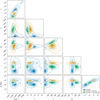 |
Fig. 1 Posterior distribution of GW-relevant parameters under the various assumptions. The contours report the 50% and 90% credibility regions. Blue posteriors were computed from GW170817 data only. Orange (green) posteriors correspond to the joint GW-kN data without (with) NR-informed mappings. |
3.2.3 Bayes factors
Within a Bayesian framework, and exploiting the nested sampling algorithm we employed above, it is immediate to compare the evidence for different hypotheses explaining the dataset under consideration, when marginalizing over the whole parameter space. Specifically, we are interested in comparing two hypotheses: the “coherent” one, in which GW and kN data are simultaneously modeled by a single common source, which we refer to as “SS” following Eq. (17), and the “incoherent” hypothesis, in which the two datasets are each explained by independent and disjoint sources, which we refer to as “DS” following Eq. (8).
The BF comparing these hypotheses can be obtained through the coherence ratio introduced in Veitch & Vecchio (2010):
 (21)
(21)
As was discussed in Veitch & Vecchio (2010) in more detail, this ratio intuitively compares the integral of the product with the product of the integrals of the distributions, a measure of how much information is gained by assuming a joint hypothesis. Additionally, we label as “SS-NR” the hypothesis obtainedwhen considering the NR-calibrated relation, Eq. (19). When applying this computation to the above results, we find that
 (22)
(22)
without assuming NR relations, and that
 (23)
(23)
when assuming NR-calibrated relations.
These results indicate that, within the available dataset and under the employed models, the two observations are better explained by the common source hypothesis (SS) only assuming NR-informed relations. An incoherent explanation (DS) is instead favored when assuming that only the distance, inclination, and coalescence time are common parameters. Since the kN model is spherical, the key parameter is the distance, but the distance is compatible among the single-messenger analyses. Thus, the negative value of  simply reflects the fact that the distance is consistent in both single-messenger analyses and a coherent analysis does not help in fitting the data more than the single-messenger analyses. Overall, this result is related to the simplified kN model used in this work and the high degeneracy in the kN parameter space discussed above. This underlines the relevance of systematics in kN modeling, and enforces the importance of informing the models with full numerical solutions by connecting them with binary parameters.
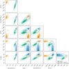 |
Fig. 2 Posterior distribution of kN relevant parameters under the various assumptions. The contours report the 50% and 90% credibility regions. Blue posteriors were computed from AT2017gfo data only. Orange (green) posteriors correspond to the joint GW-kN data without (with) NR-informed mappings. |
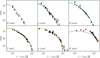 |
Fig. 3 Light curve reconstruction from the inference for AT2017gfo. The bands represent the parameter variation within their 90% credible regions. |
4 Equation of state constraints
In this section, we discuss the constraints on the EOS from our analysis. We followed an approach similar to the one presented in Breschi et al. (2021b, 2022), with a few key differences. First, we used the updated EOS-insensitive NR relations developed here. Second, we computed a new set of ~10 million phenomenological EOSs by employing minimal assumptions (Godzieba et al. 2021). The set was generated with a Markov Chain Monte Carlo approach by fixing the crust EOS and assuming only i) general relativity, and ii) causality at higher densities. Hence, it is agnostic on nuclear physics and not affected by nuclear physics uncertainties. The set includes EOSs with and without first-order phase transitions. Unlike (Godzieba et al. 2021), we did not include any constraints from GW170817 and we sampled EOSs such that  (Romani et al. 2022) a posteriori, as is described below. Third, we folded in the pulsar results from Miller et al. (2019); Vinciguerra et al. (2024). In order to consistently account for the information listed above, we sampled over the E S index in our 10 million set, iEOS, as well as over the masses of PSR J0030+0451 (MJ0030) and PSR J0740+6620 (MJ0740), and the masses of the two components of the GW170817 progenitor system (m1, m2) (Foreman-Mackey et al. 2013). Denoting
  , and dJ0740 = {MJ0740, RJ0740}, the likelihood we employed is given by
 (24)
(24)
where pMM(…), pJ0030(…), pJ0740(…) were obtained as a Gaussian Kernel Density Estimation (KDE) of posteriors from the respective analyses. Similarly, the priors on MJ0740, MJ0030, m1, m2 were obtained from their marginalized one-dimensional posterior, while the prior on the EOS index was assumed to be uniform.
The results are displayed in Fig. 4 and summarized in Table 2. The addition of kN data to the GW analysis results in a systematic shift of the  posterior to larger radii of ~0.5 km. This is essentially related to the larger
  median and, physically, to the fact that the kN places a lower bound on
  due to the disk wind (Radice et al. 2018c). The addition of the NR-informed relations to the inference has a relatively small impact on the EOS constraints, with the estimated values of
  and Λ1,4 being compatible within the error bars with the same quantities from the joint analysis. This result is not surprising, as the recovered
  and ?? distributions of the two analyses are largely consistent (see Fig. 1).
The impact of NICER data on the allowed EOSs, instead, is substantial. The permissibility of certain EOSs (e.g. MS1b) depends on the specific hotspot model employed (PDT-U or ST+PDT). The estimated distributions of  are shifted by ~1 km between the two models, indicating large systematic errors in the NICER analyses (Vinciguerra et al. 2024). Notably, while the evidence of the NICER analysis favors the PDT-U model, the hotspot configuration predicted by the ST+PDT model was found to be more consistent with the gamma-ray emission associated with PSR J0030+0451 (Kalapotharakos et al. 2021).
EOS constraints obtained from our multi-messenger PEs.
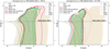 |
Fig. 4 Constraints on the EOS obtained by resampling the posteriors of the GW-only (blue), joint (red), and NR-informed joint analysis (green) using 10 million EOSs and folding in the NICER information of Vinciguerra et al. (2024), Miller et al. (2021) and the measurement of |

5 Conclusions
We have introduced bajes-MMA, a multi-messenger Bayesian pipeline for analyses of signals from BNS mergers. The key features of bajes are: (i) The use of NR relations for the ejecta mass and velocities; (ii) The use (and concurrent marginal-ization) of suitable recalibration parameters, which widen the credible ranges of inferred parameters accounting for systematic uncertainties; (iii) The possibilities of performing joint and coherent analyses. Regarding (ii), this technique has been applied here to handle the systematics of phenomenological NR relations used to link remnant properties with the binary properties. More generally, the same methodology could be employed to deal with other types of uncertainties, for example in the EOS set. We note that the open source bajes-MMA implementation is generic and can accommodate different likelihoods, datasets, and models.
Our inference results confirm previous findings on the presence of multiple kN components: a faster and lighter “dynamical” component and a slower and heavier “wind” component (Villar et al. 2017; Perego et al. 2017b; Breschi et al. 2021b). They also indicate a consistency in the source distance parameter between GW and kN data. Within spherical kN models, a common GW-kN source is favored by our joint and coherent analysis only when assuming NR-informed relations between the ejecta components and the binary parameters, which are capable of significantly breaking the correlations in the GW-kN parameter space. This result also highlights the impact of systematics in kN modeling, and that the degeneracies in the kN parameter space can be effectively reduced by incorporating the inference parametric relations with binary parameters (Raaijmakers et al. 2021b).
Multi-messenger analyses with multiple sources can help to improve mass-radius diagram constraints. Current observations of GWs and PSRs along with minimal EOS assumptions (validity of general relativity, causality) point to NS maximum masses of  with errors of ∽11% and NS radii of
  km with ~1 km uncertainty and systematics on the same order of magnitude. Our results indicate that current GW constraints are compatible with pulsar constraints, in line with other similar analyses. Pulsars constraints, however, may be particularly sensitive to systematics. For the data considered here, this is clearly the case for J0740+6620 (Vinciguerra et al. 2024). Our mass-radius constraints can be translated into pressure-density constraints for the EOS. For example, at double the saturation densities we find log P(2ρsat) = 34.61–34.76 (depending on systematics; see Table 2). Interestingly, such a constraint potentially excludes some of the EOSs commonly employed in NR simulations. Future observations of BNS might improve the precision of these constraints and also help to break systematics effects.
In order to compare our new inferences to previous work, it is useful to focus on the NS radius, which is a commonly inferred parameter. Our results are in good agreement with some of the first inferences performed on this set of data (Radice & Dai 2019; Coughlin et al. 2019) (see Fig. 12 of Breschi et al. 2021b for a collection of various results). On the one hand, we confirm the robustness of the constraint in joint and coherent analysis. On the other hand, we point out out that part of the agreement is related to the dominant effect of the minimum-maximum mass constraint from pulsar data. Additionally, our work leverages the recent pulsar analysis of Vinciguerra et al. (2024) to show that the systematics in the radius measurement from pulsar data can be significantly larger than those from GW+kN.
Future work will be devoted to exploring more sophisticated kN models like those included in the xkn framework (Ricigliano et al. 2024), as well as kN afterglow models (Hajela et al. 2020; Nedora et al. 2021b). As was discussed in Sect. 3.1, a main issue in the PE with analytical kN models appears to be the interpretation of the effective gray opacity parameters. On the one hand, it is unrealistic to expect that such a parameter can capture the complexity of the atomic physics in kN (Zhu et al. 2021; Barnes et al. 2021). On the other hand, the opacity modeling is also a significant issue when numerical models are employed (Bulla 2023). In that case, very simplified models are also employed4, but because they are not inferred, they often remain hidden in the model assumption. Overall, photon transport, hydrodynamical interaction, and atomic/nuclear physics in kN modeling remain standalone key challenges (in large part independent of Bayesian PE.)
Improved NR relations can be created by utilizing a more homogeneous set of microphysical simulations (Nedora et al. 2022) and including the contribution of the disk winds from upcoming long-term simulations Kiuchi et al. (2023); Radice & Bernuzzi (2023). This is another avenue that we plan to explore in the future.
We also plan to extend the bajes-MMA framework to include likelihood and models for GRB and afterglow data (e.g., Biscoveanu et al. 2020; Hayes et al. 2020; Farah et al. 2020; Gianfagna et al. 2023). The inclusion of this messenger can improve the inference of the extrinsic parameters of the source, in particular the viewing angle, with implications for cosmolog-ical parameters. However, the inclusion of GRB data in joint analyses is not expected to provide valuable extra information on the EOS because the link between the GRB emission and the NS matter properties is still unclear (e.g., Piran et al. 2013; Hotokezaka et al. 2018; see also Farah et al. 2020 for similar consideration of the jet structure).
Acknowledgements
S.B. acknowledges hospitality and support from the IGC at PSU, where this work was finalized. M.B. acknowledges support from the European Union’s H2020 under ERC Starting Grant, no. BinGraSp 714626; from the Deutsche Forschungsgemeinschaft (DFG) under Grant no. 406116891 within the Research Training Group (RTG) 2522/1; and from the PRO3 program “DS4Astro” of the Italian Ministry for Universities and Research. RG acknowledges support by the Deutsche Forschungsgemeinschaft (DFG) under Grant No. 406116891 within the Research Training Group RTG 2522/1 and from NSF Grant PHY-2020275 (Network for Neutrinos, Nuclear Astrophysics, and Symmetries (N3AS)) G.C. acknowledges funding from the Della Riccia Foundation under an Early Career Scientist Fellowshis, from the European Union’s Horizon 2020 research and innovation program under the Marie Sklodowska-Curie grant agreement No. 847523 ‘INTERACTIONS’, from the Villum Investigator program supported by VILLUM FONDEN (grant no. 37766) and from the DNRF Chair, by the Danish Research Foundation. S.B. acknowledges funding from the EU Horizon under ERC Consolidator Grant, no. InspiReM-101043372 and from the Deutsche Forschungsgemeinschaft, DFG, project MEMI number BE 6301/2-1. D.R. acknowledges funding from the U.S. Department of Energy, Office of Science, Division of Nuclear Physics under Award Number(s) DE-SC0021177, DE-SC0024388, and from the National Science Foundation under Grants No. PHY-2011725, PHY-2116686, and AST-2108467. The computations were performed on the ARA cluster at Friedrich Schiller University Jena, on the supercomputer SuperMUC-NG at the Leibniz- Rechenzentrum (LRZ, www.lrz.de) Munich. ARA, is a resource of Friedrich-Schiller-Universtät Jena supported in part by DFG grants INST 275/334-1 FUGG, INST 275/363-1 FUGG and EU H2020 BinGraSp-714626. The authors acknowledge the Gauss Centre for Supercomputing e.V. (www.gauss-centre.eu) for funding this project by providing computing time on the GCS Supercomputer SuperMUC-NG at LRZ (allocations pn36ge and pn36jo). This material is based upon work supported by NSF’s LIGO Laboratory which is a major facility fully funded by the National Science Foundation. Data availability: bajes is an open-source software available on GITHUB (https://github.com/matteobreschi/bajes) and on PYPI (https://pypi.org/project/bajes). For the analyses performed in this work, we employed the newly released version 1.1.0. TEOBResumS is publicly developed on BITBUCKET (https://bitbucket.org/eob_ihes/teobresums/src/master/) and available on PYPI (https://pypi.org/project/teobresums/). The GW170817 data are provided by the GWOSC (https://www.gw-openscience.org/). The AT2017gfo data are collected from Villar et al. (2017). The NICER posteriors are taken from the corresponding references, i.e. Miller et al. (2019, 2021); Riley et al. (2019, 2021); Vinciguerra et al. (2024). The EOS prior set is available on the NR-GW open data community on ZENODO (https://zenodo.org/communities/nrgw-opendata). The posterior samples presented in this work will be shared on request to the corresponding author.
Appendix A Numerical-relativity-informed relations for ejecta properties
We derived updated NR-informed EOS-insensitive relations for the dynamical ejecta mass,  , the dynamical ejecta velocity, υd, and the disk mass, mdisk. We employed the NR data collected from (Hotokezaka et al. 2013; Bauswein et al. 2013b; Dietrich et al. 2015, 2017; Lehner et al. 2016; Sekiguchi et al. 2016; Radice et al. 2018b; Vincent et al. 2020; Kiuchi et al. 2019; Perego et al. 2019; Endrizzi et al. 2020; Bernuzzi et al. 2020; Nedora et al. 2022), as it is available for each quantity. The dataset includes 262 NR simulations of non-spinning BNS mergers spanning the ranges of M ∈ [2.4,4] M⊙, q ∈ [1, 2.05], and
 ![Mathematical equation: $\tilde \Lambda \in [50,3200]$](/articles/aa/full_html/2024/09/aa49173-24/aa49173-24-eq188.png) . The ejecta data refer to simulations with different degrees of physical accuracy (Nedora et al. 2022). Some simulations do not include microphysics and/or neglect neutrino absoption, which are known to be important to describe the mass ejecta (Perego et al. 2017b). Nonetheless, we employed the entire dataset to provide a conservative constraint within the Bayesian analysis (see below).
. The ejecta data refer to simulations with different degrees of physical accuracy (Nedora et al. 2022). Some simulations do not include microphysics and/or neglect neutrino absoption, which are known to be important to describe the mass ejecta (Perego et al. 2017b). Nonetheless, we employed the entire dataset to provide a conservative constraint within the Bayesian analysis (see below).
The mass of the dynamical component was calibrated using a factorized empirical analytical form,5
 (A.1)
(A.1)
which includes effects on the symmetric mass ratio, v = m1m2 /M2,
 (A.2)
(A.2)
and in the BNS parameters,
 (A.3)
(A.3)
The coefficients, {a0, b1,2, c1,2), were calibrated on NR data using a differential evolution method. We find the optimal coefficients to be
 (A.4)
(A.4)
with χ2 = 4.91 and a standard deviation of the residuals equal to 13.6%. For the velocity of the dynamical ejecta, we employed a similar fitting formula, where the coefficients are
 (A.5)
(A.5)
with χ2 = 12.1 and a standard deviation of the residuals equal to 21 .0%. We calibrated the disk mass, mdisk, extracted from NR data using the following fitting formula:
 (A.6)
(A.6)
where, χ(Λ1 + Λ2) is a correction introduced for small Λs (Radice et al. 2018b),
![Mathematical equation: $\chi (x) = 1 + {\chi _0}\left[ {{1 \over \pi }\arctan \left( {{{x - {\Lambda _0}} \over {{\Sigma _0}}}} \right) + {1 \over 2}} \right].$](/articles/aa/full_html/2024/09/aa49173-24/aa49173-24-eq195.png) (A.7)
(A.7)
The coefficients, {a0, b1,2, c1,2,χ0, Λ0, Σ0}, were calibrated on NR data using a differential evolution method. We find the optimal coefficients to be
 (A.8)
(A.8)
with χ2 = 2.64 and a standard deviation of the residuals equal to 16.4%. As has also been shown by previous studies (Radice et al. 2018b), the total amount of disk mass increases for increasing tidal polarizability that is consequence of the small compactness of the progenitors; that is, m/R ≃ 0.1. We assume that a fraction, ξ, of the total disk mass contributes to the winds,  ·
·
 (A.9)
(A.9)
None of the relations proposed here is singular on the calibration range, and all formulas are stable in the limit Λi → 0.
As was discussed above, these NR relations carry non-negligible uncertainties, quantifiable at a level of ~20%. In order to marginalize over these theoretical uncertainties, we introduced appropriate calibration parameters, δk, in the PE. These calibration parameters affect the predictions of the dynamical ejecta properties as (Breschi et al. 2021b, 2022)
 (A.10)
 (A.11)
where the superscript “fit” denotes a prediction of an NR-informed relation. The calibration parameters, δ1,2, were assumed to be normally distributed, with variance prescribed by the residual errors. The disk mass fraction, ξ, was taken to be uniformly distributed within the range [0, 1].
References
- Acernese, F., et al. 2015, Class. Quant. Grav., 32, 024001 [NASA ADS] [CrossRef] [Google Scholar]
- Agathos, M., Zappa, F., Bernuzzi, S., et al. 2020, Phys. Rev. D, 101, 044006 [NASA ADS] [CrossRef] [Google Scholar]
- Akcay, S., Bernuzzi, S., Messina, F., et al. 2019, Phys. Rev. D, 99, 044051 [NASA ADS] [CrossRef] [Google Scholar]
- Al-Mamun, M., Steiner, A. W., Nättilä, J., et al. 2021, Phys. Rev. Lett., 126, 061101 [NASA ADS] [CrossRef] [Google Scholar]
- Anderson, W. G., Brady, P. R., Creighton, J. D. E., & Flanagan, E. E. 2001, Phys. Rev. D, 63, 042003 [NASA ADS] [CrossRef] [Google Scholar]
- Annala, E., Gorda, T., Kurkela, A., Nättilä, J., & Vuorinen, A. 2020, Nature Phys., 16, 907 [CrossRef] [Google Scholar]
- Antoniadis, J., Freire, P. C., Wex, N., et al. 2013, Science, 340, 6131 [CrossRef] [Google Scholar]
- Ayriyan, A., Blaschke, D., Grunfeld, A. G., et al. 2021, Eur. Phys. J. A, 57, 318 [NASA ADS] [CrossRef] [Google Scholar]
- Barnes, J., Kasen, D., Wu, M.-R., & Martinez-Pinedo, G. 2016, ApJ, 829, 110 [NASA ADS] [CrossRef] [Google Scholar]
- Barnes, J., Zhu, Y., Lund, K., et al. 2021, ApJ, 918, 44 [CrossRef] [Google Scholar]
- Bauswein, A., Baumgarte, T., & Janka, H. T. 2013a, Phys. Rev. Lett., 111, 131101 [NASA ADS] [CrossRef] [Google Scholar]
- Bauswein, A., Goriely, S., & Janka, H.-T. 2013b, ApJ, 773, 78 [NASA ADS] [CrossRef] [Google Scholar]
- Bauswein, A., Just, O., Janka, H.-T., & Stergioulas, N. 2017, ApJ, 850, L34 [Google Scholar]
- Bernuzzi, S., Nagar, A., Dietrich, T., & Damour, T. 2015, Phys. Rev. Lett., 114, 161103 [NASA ADS] [CrossRef] [Google Scholar]
- Bernuzzi, S., Breschi, M., Daszuta, B., et al. 2020, MNRAS, 497, 1488 [Google Scholar]
- Biscoveanu, S., Thrane, E., & Vitale, S. 2020, ApJ, 893, 38 [NASA ADS] [CrossRef] [Google Scholar]
- Brandes, L., Weise, W., & Kaiser, N. 2023, Phys. Rev. D, 107, 014011 [NASA ADS] [CrossRef] [Google Scholar]
- Breschi, M., Gamba, R., & Bernuzzi, S. 2021a, Phys. Rev. D, 104, 042001 [NASA ADS] [CrossRef] [Google Scholar]
- Breschi, M., Perego, A., Bernuzzi, S., et al. 2021b, MNRAS, 505, 1661 [NASA ADS] [CrossRef] [Google Scholar]
- Breschi, M., Bernuzzi, S., Godzieba, D., Perego, A., & Radice, D. 2022, Phys. Rev. Lett., 128, 161102 [NASA ADS] [CrossRef] [Google Scholar]
- Bulla, M. 2023, MNRAS, 520, 2558 [CrossRef] [Google Scholar]
- Capano, C. D., Tews, I., Brown, S. M., et al. 2020, Nature Astron., 4, 625 [NASA ADS] [CrossRef] [Google Scholar]
- Chornock, R., et al. 2017, ApJ, 848, L19 [NASA ADS] [CrossRef] [Google Scholar]
- Coughlin, M. W., & Dietrich, T. 2019, Phys. Rev. D, 100, 043011 [CrossRef] [Google Scholar]
- Coughlin, M. W., et al. 2018, MNRAS, 480, 3871 [NASA ADS] [CrossRef] [Google Scholar]
- Coughlin, M. W., Dietrich, T., Margalit, B., & Metzger, B. D. 2019, MNRAS, 489, L91 [NASA ADS] [CrossRef] [Google Scholar]
- Coulter, D. A., et al. 2017, Science, 358, 1556 [NASA ADS] [CrossRef] [Google Scholar]
- Cowperthwaite, P. S., et al. 2017, ApJ, 848, L17 [CrossRef] [Google Scholar]
- Cromartie, H. T., et al. 2019, Nat. Astron., 4, 72 [NASA ADS] [CrossRef] [Google Scholar]
- Damour, T., & Deruelle, N. 1986, Ann. Inst. Henri Poincaré Phys. Théor, 44, 263 [Google Scholar]
- Damour, T., & Nagar, A. 2009, Phys. Rev. D, 80, 084035 [NASA ADS] [CrossRef] [Google Scholar]
- Damour, T., & Nagar, A. 2010, Phys. Rev. D, 81, 084016 [NASA ADS] [CrossRef] [Google Scholar]
- Damour, T., Nagar, A., & Villain, L. 2012, Phys. Rev. D, 85, 123007 [NASA ADS] [CrossRef] [Google Scholar]
- Danielewicz, P., Lacey, R., & Lynch, W. G. 2002, Science, 298, 1592 [NASA ADS] [CrossRef] [Google Scholar]
- De, S., Finstad, D., Lattimer, J. M., et al. 2018, Phys. Rev. Lett., 121, 091102 [Google Scholar]
- Del Pozzo, W., & Veitch, J. 2022, CPNest: Parallel nested sampling, Astrophysics Source Code Library, [record ascl:2205.021] [Google Scholar]
- Demorest, P., Pennucci, T., Ransom, S., Roberts, M., & Hessels, J. 2010, Nature, 467, 1081 [Google Scholar]
- Dietrich, T., & Ujevic, M. 2017, Class. Quant. Grav., 34, 105014 [NASA ADS] [CrossRef] [Google Scholar]
- Dietrich, T., Bernuzzi, S., Ujevic, M., & Brügmann, B. 2015, Phys. Rev. D, 91, 124041 [NASA ADS] [CrossRef] [Google Scholar]
- Dietrich, T., Ujevic, M., Tichy, W., Bernuzzi, S., & Brügmann, B. 2017, Phys. Rev. D, 95, 024029 [NASA ADS] [CrossRef] [Google Scholar]
- Dietrich, T., Coughlin, M. W., Pang, P. T. H., et al. 2020, Science, 370, 1450 [Google Scholar]
- Endrizzi, A., Perego, A., Fabbri, F. M., et al. 2020, Eur. Phys. J. A, 56, 15 [EDP Sciences] [Google Scholar]
- Essick, R., Tews, I., Landry, P., Reddy, S., & Holz, D. E. 2020, Phys. Rev. C, 102, 055803 [NASA ADS] [CrossRef] [Google Scholar]
- Fan, Y.-Z., Han, M.-Z., Jiang, J.-L., Shao, D.-S., & Tang, S.-P. 2024, Phys. Rev. D., 109, 043052 [NASA ADS] [CrossRef] [Google Scholar]
- Farah, A., Essick, R., Doctor, Z., Fishbach, M., & Holz, D. E. 2020, ApJ, 895, 108 [NASA ADS] [CrossRef] [Google Scholar]
- Favata, M. 2014, Phys. Rev. Lett., 112, 101101 [NASA ADS] [CrossRef] [Google Scholar]
- Feroz, F., Hobson, M. P., & Bridges, M. 2009, MNRAS, 398, 1601 [NASA ADS] [CrossRef] [Google Scholar]
- Fitzpatrick, E. L. 1999, PASP, 111, 63 [Google Scholar]
- Foreman-Mackey, D., Hogg, D. W., Lang, D., & Goodman, J. 2013, PASP, 125, 306 [Google Scholar]
- Gamba, R., Bernuzzi, S., & Nagar, A. 2021a, Phys. Rev. D, 104, 084058 [NASA ADS] [CrossRef] [Google Scholar]
- Gamba, R., Breschi, M., Bernuzzi, S., Agathos, M., & Nagar, A. 2021b, Phys. Rev. D, 103, 124015 [CrossRef] [Google Scholar]
- Gianfagna, G., Piro, L., Pannarale, F., et al. 2023, MNRAS, 523, 4771 [CrossRef] [Google Scholar]
- Godzieba, D. A., Radice, D., & Bernuzzi, S. 2021, ApJ, 908, 122 [NASA ADS] [CrossRef] [Google Scholar]
- Greif, S. K., Hebeler, K., Lattimer, J. M., Pethick, C. J., & Schwenk, A. 2020, ApJ, 901, 155 [CrossRef] [Google Scholar]
- Grossman, D., Korobkin, O., Rosswog, S., & Piran, T. 2014, MNRAS, 439, 757 [NASA ADS] [CrossRef] [Google Scholar]
- Hajela, A., Margutti, R., Alexander, K. D., et al. 2020, GRB Coordinates Network, 29055, 1 [NASA ADS] [Google Scholar]
- Hayes, F., Heng, I. S., Veitch, J., & Williams, D. 2020, ApJ, 891, 124 [NASA ADS] [CrossRef] [Google Scholar]
- Hebeler, K., Lattimer, J. M., Pethick, C. J., & Schwenk, A. 2013, ApJ, 773, 11 [CrossRef] [Google Scholar]
- Hotokezaka, K., Kyutoku, K., Okawa, H., Shibata, M., & Kiuchi, K. 2011, Phys. Rev. D, 83, 124008 [NASA ADS] [CrossRef] [Google Scholar]
- Hotokezaka, K., Kiuchi, K., Kyutoku, K., et al. 2013, Phys. Rev. D, 87, 024001 [NASA ADS] [CrossRef] [Google Scholar]
- Hotokezaka, K., Beniamini, P., & Piran, T. 2018, Int. J. Mod. Phys. D, 27, 1842005 [Google Scholar]
- Huang, C., Raaijmakers, G., Watts, A. L., Tolos, L., & Providência, C. 2023, MNRAS, accepted [arXiv:2303.17518] [Google Scholar]
- Huth, S. et al. 2022, Nature, 606, 276 [CrossRef] [PubMed] [Google Scholar]
- Jaynes, E. T. 1968, in Encyclopedia of Machine Learning [Google Scholar]
- Jeffreys, H. 1939, The Theory of Probability, Oxford Classic Texts in the Physical Sciences [Google Scholar]
- Jiang, J.-L., Tang, S.-P., Wang, Y.-Z., Fan, Y.-Z., & Wei, D.-M. 2020, ApJ, 892, 1 [NASA ADS] [CrossRef] [Google Scholar]
- Kalapotharakos, C., Wadiasingh, Z., Harding, A. K., & Kazanas, D. 2021, ApJ, 907, 63 [NASA ADS] [CrossRef] [Google Scholar]
- Kashyap, R., et al. 2022, Phys. Rev. D, 105, 103022 [NASA ADS] [CrossRef] [Google Scholar]
- Kiuchi, K., Kyutoku, K., Shibata, M., & Taniguchi, K. 2019, ApJ, 876, L31 [NASA ADS] [CrossRef] [Google Scholar]
- Kiuchi, K., Fujibayashi, S., Hayashi, K., et al. 2023, Phys. Rev. Lett., 131, 011401 [NASA ADS] [CrossRef] [Google Scholar]
- Korobkin, O., Rosswog, S., Arcones, A., & Winteler, C. 2012, MNRAS, 426, 1940 [NASA ADS] [CrossRef] [Google Scholar]
- Krüger, C. J., & Foucart, F. 2020, Phys. Rev. D, 101, 103002 [CrossRef] [Google Scholar]
- Le Fèvre, A., Leifels, Y., Reisdorf, W., Aichelin, J., & Hartnack, C. 2016, Nucl. Phys. A, 945, 112 [CrossRef] [Google Scholar]
- LIGO Scientific Collaboration (Aasi, J., et al.) 2015, Class. Quant. Grav., 32, 074001 [Google Scholar]
- LIGO Scientific Collaboration and Virgo Collaboration (Abbott, B. P., et al.) 2017a, ApJ, 850, L39 [NASA ADS] [CrossRef] [Google Scholar]
- LIGO Scientific Collaboration and Virgo Collaboration (Abbott, B. P., et al.) 2017b, ApJ, 848, L13 [CrossRef] [Google Scholar]
- LIGO Scientific Collaboration and Virgo Collaboration (Abbott, B. P., et al.) 2017c, Phys. Rev. Lett., 119, 161101 [Google Scholar]
- LIGO Scientific Collaboration and Virgo Collaboration (Abbott, B. P., et al.) 2017d, ApJ, 848, L12 [NASA ADS] [CrossRef] [Google Scholar]
- LIGO Scientific Collaboration and Virgo Collaboration (Abbott, B. P., et al.) 2018, Phys. Rev. Lett., 121, 161101 [Google Scholar]
- LIGO Scientific Collaboration and Virgo Collaboration (Abbott, B. P., et al.) 2019a, Phys. Rev. X, 9, 031040 [Google Scholar]
- LIGO Scientific Collaboration and Virgo Collaboration (Abbott, B. P., et al.) 2019b, Phys. Rev. X, 9, 011001 [NASA ADS] [Google Scholar]
- LIGO Scientific Collaboration and Virgo Collaboration (Abbott, B. P., et al.) 2020, Class. Quant. Grav., 37, 045006 [NASA ADS] [CrossRef] [Google Scholar]
- Lehner, L., Liebling, S. L., Palenzuela, C., et al. 2016, Class. Quant. Grav., 33, 184002 [CrossRef] [Google Scholar]
- Margalit, B., Jermyn, A. S., Metzger, B. D., Roberts, L. F., & Quataert, E. 2022, ApJ, 939, 51 [NASA ADS] [CrossRef] [Google Scholar]
- Margalit, B., & Metzger, B. D. 2017, ApJ, 850, L19 [Google Scholar]
- Miller, M. C., et al. 2019, ApJ, 887, L24 [CrossRef] [Google Scholar]
- Miller, M. C., et al. 2021, ApJ, 918, L28 [NASA ADS] [CrossRef] [Google Scholar]
- Nagar, A., & Rettegno, P. 2019, Phys. Rev. D, 99, 021501 [NASA ADS] [CrossRef] [Google Scholar]
- Nagar, A., et al. 2018, Phys. Rev. D, 98, 104052 [NASA ADS] [CrossRef] [Google Scholar]
- Nagar, A., Riemenschneider, G., Pratten, G., Rettegno, P., & Messina, F. 2020, Rhys. Rev. D, 102, 024077 [NASA ADS] [CrossRef] [Google Scholar]
- Nedora, V., Bernuzzi, S., Radice, D., et al. 2019, ApJ, 886, L30 [NASA ADS] [CrossRef] [Google Scholar]
- Nedora, V., Bernuzzi, S., Radice, D., et al. 2021a, ApJ, 906, 98 [NASA ADS] [CrossRef] [Google Scholar]
- Nedora, V., Radice, D., Bernuzzi, S., et al. 2021b, MNRAS, 506, 5908 [CrossRef] [Google Scholar]
- Nedora, V., Schianchi, F., Bernuzzi, S., et al. 2022, Class. Quant. Grav., 39, 015008 [CrossRef] [Google Scholar]
- Nicholl, M. et al. 2017, ApJ, 848, L18 [NASA ADS] [CrossRef] [Google Scholar]
- Nicholl, M., Margalit, B., Schmidt, P., et al. 2021, MNRAS, 505, 3016 [NASA ADS] [CrossRef] [Google Scholar]
- Pang, P. T. H., et al. 2022, Nat. Com., 14, 8352 [Google Scholar]
- Perego, A., Arcones, A., Martin, D., & Yasin, H. 2017a, JPS Conf. Proc., 14, 020810 [Google Scholar]
- Perego, A., Radice, D., & Bernuzzi, S. 2017b, ApJ, 850, L37 [NASA ADS] [CrossRef] [Google Scholar]
- Perego, A., Bernuzzi, S., & Radice, D. 2019, Eur. Phys. J., A55, 124 [NASA ADS] [CrossRef] [Google Scholar]
- Perego, A., Logoteta, D., Radice, D., et al. 2022, Phys. Rev. Lett., 129, 032701 [NASA ADS] [CrossRef] [Google Scholar]
- Pian, E. et al. 2017, Nature, 551, 67 [NASA ADS] [CrossRef] [Google Scholar]
- Piran, T., Nakar, E., & Rosswog, S. 2013, MNRAS, 430, 2121 [NASA ADS] [CrossRef] [Google Scholar]
- Raaijmakers, G. et al. 2019, ApJ, 887, L22 [NASA ADS] [CrossRef] [Google Scholar]
- Raaijmakers, G., Greif, S. K., Hebeler, K., et al. 2021a, ApJ, 918, L29 [NASA ADS] [CrossRef] [Google Scholar]
- Raaijmakers, G. et al. 2021b, ApJ, 922, 269 [NASA ADS] [CrossRef] [Google Scholar]
- Radice, D., & Dai, L. 2019, Eur. Phys. J., A55, 50 [CrossRef] [Google Scholar]
- Radice, D., & Bernuzzi, S. 2023, ApJ, 959, 46 [NASA ADS] [CrossRef] [Google Scholar]
- Radice, D., & Bernuzzi, S. 2024, J. Phys. Conf. Ser., 2742, 012009 [NASA ADS] [CrossRef] [Google Scholar]
- Radice, D., Galeazzi, F., Lippuner, J., et al. 2016, MNRAS, 460, 3255 [NASA ADS] [CrossRef] [Google Scholar]
- Radice, D., Perego, A., Hotokezaka, K., et al. 2018a, ApJ, 869, L35 [NASA ADS] [CrossRef] [Google Scholar]
- Radice, D., Perego, A., Hotokezaka, K., et al. 2018b, ApJ, 869, 130 [Google Scholar]
- Radice, D., Perego, A., Zappa, F., & Bernuzzi, S. 2018c, ApJ, 852, L29 [NASA ADS] [CrossRef] [Google Scholar]
- Radice, D., Bernuzzi, S., Perego, A., & Haas, R. 2022, MNRAS, 512, 1499 [NASA ADS] [CrossRef] [Google Scholar]
- Ricigliano, G., Perego, A., Borhanian, S., et al. 2024, MNRAS, 529, 647 [NASA ADS] [CrossRef] [Google Scholar]
- Riley, T. E., et al. 2019, ApJ, 887, L21 [CrossRef] [Google Scholar]
- Riley, T. E., et al. 2021, ApJ, 918, L27 [CrossRef] [Google Scholar]
- Romani, R. W., Kandel, D., Filippenko, A. V., Brink, T. G., & Zheng, W. 2022, ApJ, 934, L17 [NASA ADS] [CrossRef] [Google Scholar]
- Rosswog, S. 2013, Philos. Trans. A, 373, 2036 [Google Scholar]
- Russotto, P., et al. 2016, Phys. Rev. C, 94, 034608 [CrossRef] [Google Scholar]
- Savchenko, V., et al. 2017, ApJ, 848, L15 [CrossRef] [Google Scholar]
- Sekiguchi, Y., Kiuchi, K., Kyutoku, K., Shibata, M., & Taniguchi, K. 2016, Phys. Rev. D, 93, 124046 [NASA ADS] [CrossRef] [Google Scholar]
- Shibata, M., Fujibayashi, S., Hotokezaka, K., et al. 2017, Phys. Rev. D, 96, 123012 [Google Scholar]
- Skilling, J. 2006, Bayesian Anal., 1, 833 [Google Scholar]
- Smartt, S. J., et al. 2017, Nature, 551, 75 [NASA ADS] [CrossRef] [Google Scholar]
- Speagle, J. S. 2020, MNRAS, 493, 3132 [Google Scholar]
- Tanaka, M., et al. 2017, PASJ, 69, 102 [NASA ADS] [CrossRef] [Google Scholar]
- Tanvir, N. R., et al. 2017, ApJ, 848, L27 [CrossRef] [Google Scholar]
- Tissino, J., Carullo, G., Breschi, M., et al. 2023, Phys. Rev. D, 107, 084037 [CrossRef] [Google Scholar]
- Valenti, S., Sand, D. J., Yang, S., et al. 2017, ApJ, 848, L24 [CrossRef] [Google Scholar]
- Veitch, J., & Vecchio, A. 2010, Phys. Rev. D, 81, 062003 [NASA ADS] [CrossRef] [Google Scholar]
- Villar, V. A., et al. 2017, ApJ, 851, L21 [CrossRef] [Google Scholar]
- Vincent, T., Foucart, F., Duez, M. D., et al. 2020, Phys. Rev. D, 101, 044053 [NASA ADS] [CrossRef] [Google Scholar]
- Vinciguerra, S., et al. 2024, ApJ, 961, 62 [NASA ADS] [CrossRef] [Google Scholar]
- Vitale, S., Del Pozzo, W., Li, T. G., et al. 2012, Phys. Rev. D, 85, 064034 [NASA ADS] [CrossRef] [Google Scholar]
- Zappa, F., Bernuzzi, S., Radice, D., & Perego, A. 2023, MNRAS, 520, 1481 [Google Scholar]
- Zhu, Y., Lund, K., Barnes, J., et al. 2021, ApJ, 906, 94 [CrossRef] [Google Scholar]
- Zhu, Z., Li, A., & Liu, T. 2023, ApJ, 943, 163 [NASA ADS] [CrossRef] [Google Scholar]
As common in the literature, we call NS radius the radius  of nonrotating, cold beta-equilibrated NS of fiducial gravitational mass 1.4 M≲. These general-relativistic equilibrium configurations are calculated by solving the Tolmann-Oppenheimer-Volkhoff equations.
In order to lighten the notation, the explicit dependency of a statistical quantity, p(x|H), on the corresponding underlying hypotheses, H, is made implicit when not necessary, i.e., p(x|H) ↦ p(x).
Note that also a different sampler from Del Pozzo & Veitch (2022) was utilized in that work.
For example, the recent analytical model of Ricigliano et al. (2024) applies the same prescription as in some numerical models (Bulla 2023); and opactities can be either prescribed or inferred.
Here, the notation log(.) indicates the natural logarithm.
All Tables
Median and 90% credible interval of relevant parameters for the different analysis configurations.
All Figures
|
Fig. 1 Posterior distribution of GW-relevant parameters under the various assumptions. The contours report the 50% and 90% credibility regions. Blue posteriors were computed from GW170817 data only. Orange (green) posteriors correspond to the joint GW-kN data without (with) NR-informed mappings. |
| In the text | |
|
Fig. 2 Posterior distribution of kN relevant parameters under the various assumptions. The contours report the 50% and 90% credibility regions. Blue posteriors were computed from AT2017gfo data only. Orange (green) posteriors correspond to the joint GW-kN data without (with) NR-informed mappings. |
| In the text | |
|
Fig. 3 Light curve reconstruction from the inference for AT2017gfo. The bands represent the parameter variation within their 90% credible regions. |
| In the text | |
|
Fig. 4 Constraints on the EOS obtained by resampling the posteriors of the GW-only (blue), joint (red), and NR-informed joint analysis (green) using 10 million EOSs and folding in the NICER information of Vinciguerra et al. (2024), Miller et al. (2021) and the measurement of |
| In the text | |
Current usage metrics show cumulative count of Article Views (full-text article views including HTML views, PDF and ePub downloads, according to the available data) and Abstracts Views on Vision4Press platform.
Data correspond to usage on the plateform after 2015. The current usage metrics is available 48-96 hours after online publication and is updated daily on week days.
Initial download of the metrics may take a while.