| Issue |
A&A
Volume 688, August 2024
|
|
|---|---|---|
| Article Number | A83 | |
| Number of page(s) | 15 | |
| Section | Numerical methods and codes | |
| DOI | https://doi.org/10.1051/0004-6361/202450450 | |
| Published online | 06 August 2024 | |
RTModel: A platform for real-time modeling and massive analyses of microlensing events
1
Dipartimento di Fisica “E.R. Caianiello”, Università di Salerno,
Via Giovanni Paolo 132,
Fisciano
84084,
Italy
e-mail: This email address is being protected from spambots. You need JavaScript enabled to view it.
2
Istituto Nazionale di Fisica Nucleare, Sezione di Napoli, Via Cintia,
Napoli
80126,
Italy
Received:
19
April
2024
Accepted:
23
May
2024
Abstract
Context. The microlensing of stars in our Galaxy has long been used to detect and characterize stellar populations, exoplanets, brown dwarfs, stellar remnants, and all other objects that may magnify the source stars with their gravitational fields. The interpretation of microlensing light curves is relatively simple for single lenses and single sources, but it becomes more and more complicated when we add more objects and take their relative motions into account.
Aims. RTModel is a modeling platform that has been very active in the real-time investigations of microlensing events, providing preliminary models that have proven very useful for driving follow-up resources towards the most interesting events. The success of RTModel comes from its ability to carry out a thorough and focused exploration of the parameter space in a relatively short time.
Methods. This modeling process is based on three key ideas. First, the initial conditions are chosen from a template library including all possible caustic crossing and approaches. The fits are then made using the Levenberg-Marquardt algorithm with the addition of a bumper mechanism to explore multiple minima. Finally, the basic computations of microlensing magnification are performed by the fast and robust VBBinaryLensing package.
Results. In this paper, we illustrate all the algorithms of RTModel in detail with the intention to foster new approaches in view of future microlensing pipelines aimed at massive microlensing analyses.
Key words: gravitational lensing: micro / methods: numerical / binaries: general / planetary systems
© The Authors 2024
 Open Access article, published by EDP Sciences, under the terms of the Creative Commons Attribution License (https://creativecommons.org/licenses/by/4.0), which permits unrestricted use, distribution, and reproduction in any medium, provided the original work is properly cited.
This article is published in open access under the Subscribe to Open model. This email address is being protected from spambots. You need JavaScript enabled to view it. to support open access publication.
1 Introduction
Microlensing is a well-established variant of gravitational lensing where the telescope resolution is insufficient to distinguish multiple images of a source or their distortion (Mao 2012). The primary observable in this context is the flux variation produced by the magnification of the source by the gravitational field of the lens moving across the line of sight. It was first suggested as a means to count dark, compact objects contributing to the budget of the Galactic dark matter (Paczynski 1986). However, it was soon discovered that microlensing is particularly sensitive to the multiplicity of the lensing objects, thanks to the existence of caustics, namely, closed curves in the source plane that bound regions in which a source is mapped in an additional pair of images (Schneider & Weiss 1986; Erdl & Schneider 1993; Dominik 1999). The light curves of binary microlensing events are then decorated with abrupt peaks at caustic crossings joined by typical “U-shaped” valleys (Mao & Paczynski 1991; Alcock et al. 1999). In addition, every time the source approaches a cusp point in a caustic, the light curve features an additional smooth peak. Such ensembles of peaks may sometimes build formidable puzzles for the microlensing modelers aiming to reconstruct the geometry and the masses of the lenses (Udalski et al. 2018).
The emergence of microlensing as a new and efficient method to detect extrasolar planets invisible to other methods has motivated continuous observation campaigns towards the Galactic bulge that have now collected more than twenty-years of data (Gaudi 2012; Tsapras 2018; Mroz & Poleski 2024). These surveys are accompanied by follow-up observations of the most interesting microlensing events with higher cadence with the purpose to catch all elusive details of the “anomalies” produced by low-mass planets around the lenses (Beaulieu et al. 2006). Given the transient nature of microlensing events, it is necessary for the maximal coverage of the light curves to avoid any gaps that could make the interpretation of the data ambiguous (Yee et al. 2018).
Driving limited follow-up resources toward interesting events requires a non-trivial real-time modeling capacity to examine a phenomenon where multiple interpretations are possible and where even the computation of one light curve is time-consuming. Several expert modelers have provided many contributions over the years with their specific codes designed for efficient searches in the microlensing parameter space with the available computational resources (Bennett & Rhie 1996; Bennett 2010; Han et al. 2024). Some of these codes have also been adapted for massive analysis of large microlensing datasets (Koshimoto et al. 2023; Sumi et al. 2023).
Among the modeling platforms contributing to a prompt classification of ongoing anomalies, RTModel stands out with a considerable number of contributions (Tsapras et al. 2014, 2019; Rattenbury et al. 2015; Bozza et al. 2016; Henderson et al. 2016; Hundertmark et al. 2018; Bachelet et al. 2019; Dominik et al. 2019; Street et al. 2019; Fukui et al. 2019; Rota et al. 2021; Herald et al. 2022). RTModel was originally designed as an extension of the ARTEMiS1 platform (Dominik et al. 2007, 2008), which provides real-time single-lens modeling of microlensing events. The original goal was to find binary and planetary models for ongoing anomalies in real-time without any human intervention. The results of the online modeling are still automatically uploaded to a website2 where they are publicly visible to the whole community. Besides real-time modeling, RTModel has also been used to search for preliminary models in a number of microlensing investigations (Bozza et al. 2012, 2016; Rota et al. 2021; Herald et al. 2022) and in the search for planetary signals in the MOA retrospective analysis (Koshimoto et al. 2023). Finally, it was in the running for the WFIRST microlensing data challenge3 (see Sec. 9), demonstrating its potential for massive data analysis.
After so many years of service, we believe that the time has come for an article fully dedicated to RTModel illustrating the algorithms that contributed to its success. Inspired by some previous studies, these algorithms contain many innovative ideas tailored on the microlensing problem. We should not forget that the code for the microlensing computation on which RTModel is based is already publicly available as a separate appreciated package with the name VBBinaryLensing (Bozza 2010; Bozza et al. 2018, 2021). This package was created within the RTModel project and is now included in several microlensing modeling platforms (Bachelet et al. 2017; Poleski & Yee 2019; Ranc & Cassan 2018). In addition, the whole RTModel code has been completely revised and cleaned up and has been made public on a dedicated repository4. This paper will provide a detailed description of the algorithms behind this software as a reference for users and a possible inspiration for further ideas and upgrades in view of future massive microlensing surveys.
The paper is structured as follows. Section 2 explains the global architecture of RTModel, with a presentation of the different modules. Section 3 deals with the pre-processing of the datasets. Section 4 illustrates the choice of initial conditions for fitting. Section 5 discusses the fitting algorithm. Section 6 shows the selection of models and the removal of duplicates. Section 7 illustrates the sequence of operations taken to explore different model categories including higher order effects. Section 8 describes the final classification of the microlensing event and the assignment to a specific class. Section 9 discusses the success rate reached in the WFIRST data challenge as a specific example demonstrating the efficiency of RTModel on a controlled sample. Section 10 contains the conclusions.
2 General architecture of RTModel
RTModel is in the form of as a standard Python package regularly importable by Python scripts or Jupyter notebooks. It is made up of a master program calling a number of external modules for specific tasks. The communication between modules is ensured by human readable ASCII files. This allows for an easy control of the flow and possible manual interventions if needed. Furthermore, in case of any interruptions before the conclusion of the analysis, the master program is able to automatically recover all partial results and continue the analysis up to the full completion.
While the master program is in Python, the external modules are written in C++ language for higher efficiency. The individual modules can also be launched separately by the user, if desired. A list of modules called by the RTModel master program is given below, along with a brief description.
Reader: data pre-processing, including cutting unneeded baseline, re-binning, re-normalization of the error bars, and rejection of outliers.
InitCond: initial conditions setting, obtained by matching the peaks found in the photometry to the peaks of templates in a fixed library.
LevMar: fitting models from specific initial conditions by the Levenberg-Marquardt algorithm; multiple solutions are obtained by a bumper mechanism.
ModelSelector: selection of best models of a given class and removal of duplicates.
Finalizer: interpretation of the microlensing event obtained by comparing the chi squares of the found models following Wilks’ theorem.
Each of these modules is discussed in detail in a dedicated section in the following text. Figure 1 shows the flow chart of RTModel: the master program calls the individual modules one by one. Each module takes some specific data as input and provides some output that is then used by the following modules. The two modules in the orange box are repeated for each model category (single lens, binary lens, etc.)
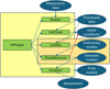 |
Fig. 1 Flow chart of RTModel with the different modules in green and the data and/or products in blue ovals. The orange box highlights the modules that are called repeatedly for each model category with their respective products. |
3 Data pre-processing
The photometric series from different telescopes can be quite inhomogeneous, with different levels of scatter that might not be reflected by the reported error bars. Without any corrections, there is the danger that the fit is dominated by poor datasets with unrealistically small error bars. Furthermore, some data may still contain outliers that may alter the whole modeling process. On the other hand, some datasets may bring redundant data that add no useful information but slow down the fit process. The Reader module takes care of all these aspects and tries to combine all the available photometry assigning the right weight to each data point as described below.
There should be one input file per photometric series (identified by its telescope and filter). For each data point, the input file should contain the magnitude (instrumental or calibrated), the error, and the time in Heliocentric Julian Date format (HJD). The datasets are first loaded and time-ordered. It is possible to consider data from all years, to take into account multi-year baselines, or focus on one year only (if the multi-year baseline is not reliable).
 |
Fig. 2 Assessment of scatter in the photometry. The green point is one-sigma above extrapolation from the two preceding points and half-sigma from the extrapolation of the two following points. |
3.1 Scatter assessment
The scatter in each dataset is estimated by summing the residuals of each point from linear extrapolation of the two previous points and the two following points (see Fig. 2). The residual is then down-weighted exponentially with time-distance. We can show this in the form of quantitative formulae as follows.
If fi is the flux of the i-th point in the photometric series, σi is its error, and ti is the time of the measurement, we consider the residual from extrapolation of the previous two points as:
![Mathematical equation: $\[r_i^{-}=\left(\frac{\Delta_i^{-}}{\sigma_i^{-}}\right)^2 w_i^{-},\]$](/articles/aa/full_html/2024/08/aa50450-24/aa50450-24-eq1.png) (1)
(1)
where the difference from the extrapolation is (see Fig. 2):
![Mathematical equation: $\[\Delta_i^{-}=f_i-\left[f_{i-2}+c_i\left(f_{i-1}-f_{i-2}\right)\right],\]$](/articles/aa/full_html/2024/08/aa50450-24/aa50450-24-eq2.png) (2)
(2)
with a linear extrapolation coefficient
![Mathematical equation: $\[c_i=\frac{t_i-t_{i-2}}{t_{i-1}-t_{i-2}},\]$](/articles/aa/full_html/2024/08/aa50450-24/aa50450-24-eq3.png) (3)
(3)
and the error in the extrapolation is obtained by error propagation as:
![Mathematical equation: $\[\sigma_i^{-}=\sqrt{\sigma_i^2+\sigma_{i-1}^2 c_i^2+\sigma_{i-2}^2\left(1-c_i\right)^2}.\]$](/articles/aa/full_html/2024/08/aa50450-24/aa50450-24-eq4.png) (4)
(4)
The residual is further weighted by
![Mathematical equation: $\[w_i^{-}=\exp \left[-\left(t_i-t_{i-2}\right) / \tau\right],\]$](/articles/aa/full_html/2024/08/aa50450-24/aa50450-24-eq5.png) (5)
(5)
so as to avoid using information from too far points, where extrapolation no longer any sense. The constant τ is set to 0.1 days since, in most cases, we do not expect features lasting less than a few hours in microlensing. Even if they are present (e.g., at a caustic crossing), such features are isolated and do not contribute much to the total scatter that would still be dominated by the overall behavior of the dataset.
Similar expressions hold for the residual, ![Mathematical equation: $\[r_i^{+}\]$](/articles/aa/full_html/2024/08/aa50450-24/aa50450-24-eq6.png) , calculated from the extrapolation of the two following points.
, calculated from the extrapolation of the two following points.
The average scatter of the dataset is then:
![Mathematical equation: $\[S=\sqrt{\frac{1+\sum\left(r_i^{-}+r_i^{+}\right)}{1+\sum\left(w_i^{-}+w_i^{+}\right)}}.\]$](/articles/aa/full_html/2024/08/aa50450-24/aa50450-24-eq7.png) (6)
(6)
The unity is added so as to avoid instabilities for too sparse datasets (which would come up with vanishing weights). For these, in fact, our assessment on the intrinsic scatter would be impossible.
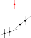 |
Fig. 3 Identification of an outlier: if the extrapolations from the preceding and following points agree, a threshold is set for the residual of the current point. Beyond this threshold, the point is removed as outlier. |
3.2 Outliers removal
The residual from the extrapolations from previous and following points is also useful to identify and remove outliers. If the two extrapolations agree better than ![Mathematical equation: $\[3 \sqrt{\left(\sigma_i^{-}\right)^2+\left(\sigma_i^{+}\right)^2}\]$](/articles/aa/full_html/2024/08/aa50450-24/aa50450-24-eq8.png) , while the residuals exceed a user-defined threshold (default value is 10), the point is identified as outlier and removed from the dataset. In detail, the condition is
, while the residuals exceed a user-defined threshold (default value is 10), the point is identified as outlier and removed from the dataset. In detail, the condition is ![Mathematical equation: $\[\sqrt{\left(r_i^{-}\right)^2+\left(r_i^{+}\right)^2}>\text { thr }_{\text {outliers }}\]$](/articles/aa/full_html/2024/08/aa50450-24/aa50450-24-eq9.png) . We refer to Fig. 3 for a pictorial view.
. We refer to Fig. 3 for a pictorial view.
3.3 Error bar re-scaling
In the end, the error bars are rescaled by the factor S, tracking the average discrepancy between each point and the extrapolations from the previous or subsequent points. The error bar re-scaling proposed in Reader is particularly sensitive to datasets with large scatter on short timescales. Unremoved outliers contribute to the increase of the error bars if they occur close to other data points. Scatter on longer timescales is more difficult to identify without a noise model. At this early stage, where we are looking to find preliminary models for a microlensing event, it is premature to take a more aggressive approach. Optionally, error bar re-scaling can be turned off if all datasets are believed to have correct error bars.
3.4 Re-binning
One of the goals of RTModel is to provide real-time assessment of ongoing microlensing events. The computational time grows linearly with the number of data points, but sometimes we have a huge number of data points on well-sampled sections of the light curve. Baseline data points also increase the computational time, but their information could be easily taken into account by just using a few points.
The idea pursued by Reader in order to speed up calculations is to replace redundant data points by their weighted mean. Data are consequently binned down to a specified number of data points. The target number can be specified by the user depending on the available computational resources and the specific problem.
The re-binning proceeds according to a significance indicator that is calculated for each pair of consecutive data points in a given dataset and estimated as:
![Mathematical equation: $\[Y_i=\frac{\left(f_i-f_{i-1}\right)^2}{\sigma_i^2+\sigma_{i-1}^2}+\frac{\left(t_i-t_{i-1}\right)^2}{\tau^2}.\]$](/articles/aa/full_html/2024/08/aa50450-24/aa50450-24-eq10.png) (7)
(7)
In practice, a consecutive pair of data points has low significance if the difference between the two points is less than their combined uncertainty and they are closer than the time threshold, τ, as already mentioned above in the context of scatter assessment. The pair with the lowest significance in all datasets is then replaced by a weighted mean. The significance of the new point in combination with the preceding one and the following one are re-calculated and the re-binning procedure is repeated until we are left with the desired number of points. Optionally, the significance of points that are outside the peak season (identified as the season in which the highest standard deviation is achieved) can be severely down-weighted. In this way, baseline points are strongly re-binned and computational time is saved for more interesting points.
Figure 4 shows an example of re-binning on a simulated event. We can see that the fundamental points describing the anomaly are preserved, while some other points where the light curve is not changing rapidly are replaced by re-binned versions along with their neighbors.
There are certainly events for which an overly aggressive rebinning leads to the smoothing of tiny features in the anomaly. Typical examples are high-magnification events with many data points on the peak that are important to assess the presence of planets tracked by perturbations of the central caustic. Thus, rebinning must be used with moderation and keeping in mind that it has been originally introduced with the purpose of guaranteeing preliminary models in a short and definite time. Nevertheless, the same philosophy of real-time modeling applies to the analysis of massive datasets as long as the purpose remains the same, namely, a first assessment of the nature of the microlensing event. Tests on the data challenge light curves (Sec. 9) confirm that the computational timescales linearly with the specified number of points that are left after re-binning. Both error bar rescaling and re-binning can be tuned to have the best performance for the specific datasets to be analyzed or can be easily turned off by the user.
The final outcome of Reader is a single ASCII file containing all data labeled according to their original datasets. Data taken from satellites also carry a satellite number, which will be used by the fitting module to identify them and perform the correct computation.
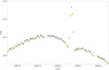 |
Fig. 4 Re-binning at work on a simulated event. Points from the original data untouched by re-binning are in green. Original points replaced by their re-binned versions with neighbors are in blue, new points resulting from re-binning are in yellow. |
4 Setting up the initial conditions
The strategy of RTModel for binary microlensing modeling is to start the fits from a finite set of initial conditions described by a template library following a philosophy initially introduced by Mao & Di Stefano (1995) and pursued by Liebig et al. (2015) in their systematic search of light curve classes in binary microlensing. Such templates must be matched to the observed data points in order to set the initial values of the parameters for the fits. These tasks are performed by the dedicated module InitCond, which operates in two phases: identification of peaks in the data, template matching.
We go on to discuss these two steps in this section focusing on the basic models with no higher order effects. We leave the discussion of parallax, xallarap, and orbital motion to Sec. 7.
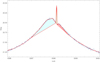 |
Fig. 5 Spline model for a simulated dataset. Concave sections are also highlighted with different colors. |
4.1 Identification of peaks in the data
Template matching is achieved by matching two peaks in the template to two analogous features in the data. So, the purpose of this stage is to find the times, t1 and t2, of the two most prominent peaks in the data. In the absence of a second well-defined peak, a shoulder or an asymmetry in the light curve could then be considered as an embryo of a peak that with a small change in the parameters would become a real peak. The following steps are aimed at identifying such features.
Spline modeling. Each dataset is modeled by a linear spline in the following way. We start with a flat line at the mean flux level. Then we add the point with the highest residual from this line to the spline model. We continue adding points to the spline model until there are no points with a residual higher than a chosen threshold (5σ as default). The spline model so obtained serves as basis for the identification of peaks and shoulders in the following steps. Figure 5 shows an example of spline derived in this way from a simulated dataset.
Concavities and convexities. A concavity is a point in the spline model standing above the line connecting the previous and following point in the spline. A convexity is a point standing below such a line. Consecutive concavities (convexities) define a concave (convex) section of the spline model. In Fig. 5, the concave sections are highlighted with different filling colors.
Peaks and shoulders. Within a concave section of the spline, we identify one peak as the highest point internal to the concave section. If the highest point is at the boundary of the section, then the section contains no peaks. In this case, we identify a “shoulder” as the point with the maximal residual from the line connecting the left and right boundary of the concave section. Such a shoulder is then treated similarly to other peaks.
Each peak or shoulder is assigned a left and right uncertainty calculated using the position of the first points in the concave section that would bring down the residual of the peak below a given threshold (5σ in default options) if they were to replace the boundaries of the section. If no points satisfy this criterion, the left and right uncertainties are defined by the boundaries of the concave section.
Prominence of the peaks. The highest peak is assigned a prominence as the number of sigmas distinguishing it from the global minimum of the dataset. The other peaks are assigned a prominence with respect to the local minimum (if any) separating them from the highest peak. Shoulders are assigned a prominence with respect to the line connecting the boundaries of their concave section.
Cross-matching peaks in different datasets. The above procedure is performed separately on each available dataset. At this point, we have a separate list of peaks for each dataset. The next task is to cross-match these lists.
We first identify peaks as the same in different datasets whose positions fall within the uncertainty range of each other. Such duplicate peaks are replaced by a single peak with an uncertainty range defined as the intersection of the two original uncertainty ranges and the prominence taken as the sum of the prominences of the two peaks.
As a second step, we also identify peaks as the same in which only one of the peak positions falls in the uncertainty range of the other peak. This is a weaker condition that is applied only after the first condition has already been used to refine all well-identified peaks. Finally, all peaks with prominence below a chosen threshold (10σ in default options) are removed.
Peak selection. In the end, we save the positions t1 and t2 of the two peaks with the highest prominence as defined above. It is evident that one of these peaks may also be a shoulder to a main peak, provided they are separated by a convex section of the spline.
Maximal asymmetry. If this algorithm only finds one peak and no shoulders, for each dataset we calculate the deviation of each point in the spline models from the symmetric spline model obtained by reflecting the spline around the position of the lonely peak found. The maximal positive deviation is then taken as the second peak.
The procedure described here and adopted by InitCond is very effective for well behaved datasets and allows for the detection of features in the data that are above the prescribed threshold. Noise in the baseline may produce spurious peaks that can be removed by increasing the overall peak threshold.
4.2 Initial conditions for Single-lens-single-source models
Single-lens-single-source microlensing events depend solely on three minimal parameters: the time of closest approach, t0, the Einstein time, tE, fixing the timescale of the event, and the impact parameter, u0, determining the peak magnification. By default, we also fit for the source size ρ* in units of the Einstein radius, θE, which is, however, seldom constrained in microlensing events.
Once we have found the two most prominent peaks, t1 and t2, from the previous algorithm, for single-lens-single-source events, we just take t0 = t1, namely, we identify the position of the highest peak as the closest approach time between source and lens. The second peak-shoulder-asymmetry is ignored in these fits. All remaining parameters u0, tE, ρ* are taken from a grid since fitting of this class of models is so fast and the number of parameters is sufficiently small that this strategy remains the most efficient.
4.3 Initial conditions for single-lens-binary-source models
For single-lens binary source models, we have to duplicate the closest approach time and the impact parameters. We naturally take t0,1 = t1 and t0,2 = t2, namely, we match the positions of the two peaks identified in the previous step to the closest approach times between each source and the lens. One more parameter is the flux ratio between the two sources, qf. Furthermore, in principle, also the secondary source has its own finite radius, but it is convenient to calculate it from the radius of the primary source and rescale it by some luminosity-radius relation in order to enforce consistency with the flux ratio. The choice ![Mathematical equation: $\[\rho_2=\rho_1 q_f^{0.225}\]$](/articles/aa/full_html/2024/08/aa50450-24/aa50450-24-eq11.png) is just one among popular choices depending on the section of the main sequence we are considering. Whatever the relation used, it would be quite exceptional that both sources show finite-size effect at the same time. So, the particular choice of this relation is not expected to have any impact on the general model search performed by RTModel. Similarly to single-source models, the parameters u0,1, u0,2, tE, ρ*, qf are again taken from a grid.
is just one among popular choices depending on the section of the main sequence we are considering. Whatever the relation used, it would be quite exceptional that both sources show finite-size effect at the same time. So, the particular choice of this relation is not expected to have any impact on the general model search performed by RTModel. Similarly to single-source models, the parameters u0,1, u0,2, tE, ρ*, qf are again taken from a grid.
4.4 Initial conditions for binary-lens-single-source
In this case, we have three more parameters with respect to the single-lens case: the mass ratio between the two lenses q, the separation s in units of the Einstein angle, the angle α between the vector joining the two lenses (oriented toward the more massive one) and the source direction. We also notice that t0 and u0 are the closest approach parameters defined with respect to the center of mass of the lens.
For binary lens models we use a template library currently made up of 113 different n-ples of parameters. Each template is characterized by its parameters s, q, u0, α, ρ*. For each template we have pre-calculated the positions of two peaks in units of the Einstein time tp1, tp2. The templates are chosen as representative light curves for regions in the parameter space in which the peaks have the same nature (same fold crossing or same cusp approach) (Liebig et al. 2015). These templates including all caustic topologies, different mass ratios and different orientations of the source trajectory. Their parameters are listed in Table A.1. The idea is that the observed microlensing light curve should necessarily belong to one of these classes and, thus, the fit from a template in the same class should proceed without meeting any barriers in the chi square surface.
Therefore, for each template in the library, we set the initial conditions by copying the five parameters in the template, save for tE and t0, which are determined by matching the peaks in the template tp1, tp2 to the peak positions t1, t2 as found by the peak identification algorithm:
![Mathematical equation: $\[t_E=\frac{t_2-t_1}{t_{p 2}-t_{p 1}},\]$](/articles/aa/full_html/2024/08/aa50450-24/aa50450-24-eq12.png) (8)
(8)
![Mathematical equation: $\[t_0=t_1-t_E t_{p 1}.\]$](/articles/aa/full_html/2024/08/aa50450-24/aa50450-24-eq13.png) (9)
(9)
We have two possible ways to match such times for each template (we may match t1 to tp1 and t2 to tp2 or exchange the two times). In one of the two cases we obtain a negative tE, which is equivalent to inverting the source direction α and the sign of u0. We finally end up with 226 different initial conditions for static binary lens models.
Figure 6 illustrates how template matching works in initial conditions setting. Here, we have some simulated data and one of the templates is matched to the data by using the main peaks, which in this case are caustic crossing peaks. With initial conditions set in this way, we are confident that at least one of the templates falls in the same light curve category of the observed event, so that the following fit will very quickly converge to the correct solution.
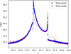 |
Fig. 6 Example of template matching to some simulated data using template # 47. |
4.5 Initial conditions for small planetary anomalies
The templates listed in Table A.1 cover all caustic topologies and source trajectories starting from mass ratios closer to 1, which are appropriate for stellar binaries. Although all planetary microlensing light curves are in principle reachable from these templates, the fitting algorithm needs to move a long way to reach such distant corners of the parameter space. As a boost for efficiency in the planetary regime, we also included further initial seeds determined along the lines initially proposed by Gould & Loeb (1992; see also Gaudi & Gould 1997; Bozza 1999; Han 2006; Gaudi 2012; Zhang & Gaudi 2022). This strategy starts from the parameters of the best models found from the single-lens-single-source search to inject the planetary perturbation at the position of the anomaly. It can only be implemented after the fits of the single-lens-single-source models and then these further initial seeds are not calculated in the InitCond module, but in the ModelSelector (see Sec. 6).
In practice, the parameters t0, tE, u0 are taken from the single-lens-single-source model. The parameter ρ* is set to 0.001 because we want to be as sensitive as possible to minor anomalies. The mass ratio is initially set to q = 0.001, well in the planetary regime.
The other parameters are then obtained by requiring that the planet generates a peak in the position of the second peak t2 as found by InitCond. In particular, we first calculate the abscissa of the anomaly along the trajectory
![Mathematical equation: $\[\widehat{d t}=\frac{t_2-t_0}{t_E}.\]$](/articles/aa/full_html/2024/08/aa50450-24/aa50450-24-eq14.png) (10)
(10)
Then we find the angular distance of the anomaly from the primary lens:
![Mathematical equation: $\[x_a=\sqrt{u_0^2+\widehat{d t}^2}.\]$](/articles/aa/full_html/2024/08/aa50450-24/aa50450-24-eq15.png) (11)
(11)
Then we have the angle between the closest approach point and anomaly point:
![Mathematical equation: $\[\alpha_0=\arctan \frac{u_0}{-\widehat{d t}}.\]$](/articles/aa/full_html/2024/08/aa50450-24/aa50450-24-eq16.png) (12)
(12)
Now, we can distinguish the cases for close- and wide-separation planets.
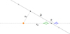 |
Fig. 7 Determination of initial conditions for planetary fits in the wide configuration. The blue caustic comes with the choice s = s+ and the green caustic with s = s−. |
4.5.1 Wide-separation planets
A wide-separation planet would produce a planetary caustic at distance, xa, if its separation is:
![Mathematical equation: $\[s_0=\frac{1}{2}\left[\sqrt{4+x_a^2}+x_a\right].\]$](/articles/aa/full_html/2024/08/aa50450-24/aa50450-24-eq17.png) (13)
(13)
We then decrease q until the size of the planetary caustic (calculated as in Bozza 2000; Han 2006) is smaller than the separation from the primary, namely, we require ![Mathematical equation: $\[x_a<4 \sqrt{q} / s_0^2.\]$](/articles/aa/full_html/2024/08/aa50450-24/aa50450-24-eq18.png) .
.
At this point, we just choose the separation of the planet in such a way that the planetary caustic is either just within or beyond the anomaly point:
![Mathematical equation: $\[s_{ \pm}=s_0 \pm \frac{4 \sqrt{q}}{s_0^2},\]$](/articles/aa/full_html/2024/08/aa50450-24/aa50450-24-eq19.png) (14)
(14)
and take α = α0 to fix all 7 parameters for the binary-lens model.
The two values s± cover the inner/outer degeneracy typical of wide-separation planets (Zhang & Gaudi 2022). Figure 7 shows the two initial conditions obtained with this approach in a practical case, illustrating the geometric quantities introduced in this subsection.
4.5.2 Close-separation planets
For close-separation planets, a caustic in xa is obtained for:
![Mathematical equation: $\[s_0=\frac{1}{2}\left[\sqrt{4+x_a^2}-x_a\right].\]$](/articles/aa/full_html/2024/08/aa50450-24/aa50450-24-eq20.png) (15)
(15)
Again, we decrease q until the size of the planetary caustic is less than the separation from the primary, namely, we require ![Mathematical equation: $\[x_a<2 * \sqrt{(}q) / s_0\]$](/articles/aa/full_html/2024/08/aa50450-24/aa50450-24-eq21.png) (Bozza 2000; Han 2006).
(Bozza 2000; Han 2006).
For close-in planets we fix the separation s = s0, but we choose two values of α as:
![Mathematical equation: $\[\alpha_{ \pm}=\alpha_0+\pi \pm \arcsin \left|\frac{2 \sqrt{q}}{s x_a}\right| \text {, }\]$](/articles/aa/full_html/2024/08/aa50450-24/aa50450-24-eq22.png) (16)
(16)
which make the anomaly point in t2 lie within or beyond one of the triangular caustics (note that t2 is the time of a peak not a trough).
The two seeds obtained in this way are illustrated in Fig. 8. Also, in this case, we cover the inner/outer degeneracy. In total, for each single-lens-single-source model passing the ModelSelector selection, we have four additional initial conditions for binary-lens fits specifically placed in the planetary regime.
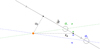 |
Fig. 8 Determination of initial conditions for planetary fits in the close configuration. The blue caustic comes with the choice α = α+ and the green caustic with α = α−. |
5 Fitting
For each starting point, as proposed by the initial conditions algorithm described in the previous section, we perform a downhill fit by Levenberg-Marquardt (LM) algorithm (Levenberg 1944; Marquardt 1963) to find a local minimum of the chi square function. This is carried out by launching the dedicated module LevMar, which fits a specific model (single-lens-single-source, single-lens-binary-source, and binary-lens-single-source) from the chosen initial condition. Since we have a large number of initial conditions to test, it is convenient to launch many LevMar processes in parallel, exploiting the available cores. This is automatically managed by the main RTModel module, which launches a new process whenever one of the previous ones has terminated.
The total computation time needed for modeling one microlensing event roughly scales with the inverse of the number of the available cores. It is, however, possible that one of the processes ends up in a region in which the computation becomes extremely slow (huge sources, extremely long Einstein times). For general purpose modeling, it is possible to set a time limit to avoid getting stuck because of these extreme regions of the parameter space. If the user believes that such regions need to be probed in depth, the time limit can be relaxed accordingly.
5.1 The Levenberg-Marquardt (LM) algorithm
The LM algorithm interpolates between steepest descent and Gauss-Newton’s algorithm adaptively. The steepest descent just takes a step in the direction opposite to the gradient of the chi square function, whereas the Gauss-Newton’s method attempts a parabolic fit of the chi square function and directly suggests the position of the local minimum. In principle, Gauss-Newton’s method is a second-order method that is much more efficient than steepest descent. However, if we are still too far from the minimum, the parabolic approximation may be very poor and lead to weird suggestions. In the LM approach, a control parameter λ modifies the set of equations that provide the step to the next point. When λ is small, the equations behave like in Gauss-Newton, whereas the set becomes equivalent to steepest descent when λ is large. The algorithm starts with an intermediate value of λ and if the suggested point improves the chi square then λ is lowered by a fixed factor. If the suggested point is worse than the previous one, λ is increased until the suggested point improves the chi square.
The LM algorithm is very efficient in dealing with complicated chi square functions such as those characterizing microlensing. In fact, it is able to follow long valleys in the chi square surface adapting the step size to the local curvature and then rapidly converge to the minimum when it gets close enough. Of course, each step needs the evaluation of the local gradient, which requires numerical derivatives for each non-linear parameter. Therefore, the total number of microlensing light curves to be calculated is (1 + p + a)Nsteps, where p is the number of nonlinear parameters, Nsteps is the number of steps to achieve the convergence threshold, and a is the average number of adjustments to the λ parameter per step, which is on the order of one.
As stopping conditions for our fits we set a default (but customizable) maximum number of 50 steps or three consecutive steps with a relative improvement in χ2 lower than 10−3χ2. In general, the latter condition is met in most fits well before the 50 steps, which only affect fits starting very far from minima. For each minimum found, we also report the local covariance ellipsoid calculated through inversion of the Fisher matrix. This is also used in model selection to identify and remove duplicates (see Sec. 6).
5.2 Microlensing computations
All models are calculated by the public package VBBinaryLensing (Bozza 2010; Bozza et al. 2018, 2021), which is now a separate popular spin-off of the original RTModel project5. Indeed, most of the credits for the efficiency of RTModel come from the fast and robust calculations provided by this package. On the other hand, in more than ten years of service, RTModel has ensured that the VBBinaryLensing package has been tested on an extremely large variety of microlensing events, enhancing its reliability.
In short, VBBinaryLensing uses pre-calculated tables for single-lens calculations with finite source effect and the contour integration algorithm (Dominik 1995, 1998; Gould & Gaucherel 1997) for binary lenses. The idea is to sample the source boundary and invert the binary lens equation in order to obtain a sampling of the images boundaries. The inversion of the lens equation is performed by the Skowron & Gould algorithm (Skowron & Gould 2012). The sampling of the source boundary is driven by accurate error estimators that select those sections that need denser sampling. The accuracy is greatly improved by parabolic corrections, while limb darkening is taken into account by repeating the calculation on concentric annuli. The number and location of the annuli is also chosen dynamically on the basis of error estimators (Bozza 2010). Since finite-size calculations are computationally expensive, the code starts with a point-source evaluation and estimates the relevance of finite-source corrections by the quadrupole correction and tests on the ghost images (Bozza et al. 2018). More recently, also the computation of the astrometric centroid has been added to VBBinaryLensing (Bozza et al. 2021) and will be incorporated in future releases of RTModel for simultaneous fitting of photometric and astrometric microlensing.
RTModel also inherits all specific techniques for higher order effect computations from VBBinaryLensing, including parallax, binary-lens orbital motion, or binary-source xallarap. In particular, for space-based datasets, which have been marked by a satellite number in the data pre-processing phase (see Sec. 3), the source is displaced according to the microlensing parallax vector components, using knowledge of the satellite position at the time of the observation (Gould 1992). This is derived from ephemerides tables that can be easily downloaded by the user from the NASA Horizon website6.
5.3 Exploring multiple minima
As stated before, the optimization problem in microlensing is complicated by the high dimensionality of the parameter space and the existence of caustics, which generate complicated barriers and valleys in the χ2 surface. The library of initial conditions presented in Sec. 4 ensures that at least one initial condition is in the correct region of the parameter space, with the same sequence of peaks and minima as the true solution. However, this is not always enough to guarantee that the correct initial condition will converge to the global minimum. In fact, accidental degeneracies due to the sampling in the data may fragment the correct region of the parameter space into multiple minima. Furthermore, the path to the global minimum may pass through extremely thin valleys surrounded by high barriers. Such valleys typically slow down the LM algorithm, which will take too many steps to converge, eventually stopping before the true minimum has been reached.
The optimization for functions that are not globally convex is characterized by a very long history that has been amply covered in the literature and so, we do not explore it further in this work. The strategy that we adopted to broaden our search and avoid stopping at the first local minimum is a Tabu-search type (Glover 1989, 1990), which avoids solutions visited in the past.
Whenever a local minimum x0 is found by the LM algorithm, a “bumper” is placed in its position that will repel new fits from the minimum found. The bumper is first defined to coincide with the covariance ellipsoid centered on the local minimum, calculated through the inversion of the Fisher matrix. As the LM is repeated from the same initial condition, it will end up in a point x in the bumper region. At this point, the bumper will push the fit outside its ellipsoid region according to the following rule:
![Mathematical equation: $\[\boldsymbol{\hat{x}=x}-2 p \frac{\boldsymbol{\Delta x}}{\sqrt{\boldsymbol{\Delta x}^T \hat{A} \boldsymbol{\Delta x}}},\]$](/articles/aa/full_html/2024/08/aa50450-24/aa50450-24-eq23.png) (17)
(17)
where Δx = x − x0 is the vector from the bumper center to the current position of the fit x; Â is the curvature matrix in x0, namely, the inverse of the covariance matrix; also, p is a coefficient that can be chosen by the user (initially set to 2).
With this push, the fit is sent outside the covariance ellipsoid of the minimum, but in general this is not sufficient to exit the attractor basin of the minimum. The bumper size is then increased by a fixed factor dividing the curvature Â, so that if the fit comes back close to the same minimum, it receives another push that brings it further way. Eventually, the fit will exit the attractor basin and converge to some other minimum (if any).
Figure 9 illustrates the bumper mechanism. We note that the minus sign in Eq. (17) pushes the fit across the minimum to the other side. In principle, we could have made the opposite choice and bump the fit away from the minimum along the Δx vector or even bump to a random direction. Our specific choice comes from the fact that a common situation occurring in the fitting is that the fit is following some long valley but gets stuck in a local minimum. Yet the true minimum is just beyond this local minimum. Therefore, in the next attempt, we want to pass beyond this minimum rather than being bounced back. Indeed, in our experience, we find that this choice is sensibly more productive in terms of new minima found.
Figure 10 illustrates the benefit of the bumper mechanism by showing fitting tracks starting from the same initial seed. The first fit (red track) gets stuck in a local minimum, but the second fit jumps out of the minimum thanks to the bumper mechanism and more minima are found with much lower chi square. The number of minima to be found from the same initial seed can be chosen by the user as usual (5 is the default choice).
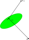 |
Fig. 9 Bumper mechanism to jump out of local minima. The fit coming from x−1 ends in x, within the covariance ellipsoid of the previously found minimum x0. It is then bumped to |
![Mathematical equation: $\[\hat{\mathbf{x}}\]$](/articles/aa/full_html/2024/08/aa50450-24/aa50450-24-eq24.png)
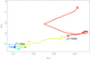 |
Fig. 10 Fit track obtained on some simulated data projected to the plane (ln s, ln q) in a binary-lens fit. We see that the first fit (red track) ended at a local minimum with high χ2. Then, repeating the fit with the bumper mechanism leads to a different region with a much lower χ2, where some more minima are found. |
6 Model selection
With so many initial conditions and the possibility to search for multiple minima from the same initial condition (as explained in Sec. 5.3), RTModel accumulates a large number of models for each class. For example, for static binary lenses, we have 226 initial conditions producing many minima each (5 with the default settings explained above). The ModelSelector module is designed to vet these models, remove duplicates, check for all possible reflections, and retain the most interesting models.
First of all, we consider two models with similar parameters as duplicates if their uncertainty ellipsoids (obtained by the covariance matrix) overlap. This criterion is very simple and allows us to remove minima found by two different fits. However, it is still possible that models lying along a valley with high enough curvature in the parameter space survive this cut. At the level of preliminary model search, it is not a bad idea to retain such closely related models for following detailed local searches using MCMC. In fact, starting a Markov chain from two different points in the same valley is a recommended sanity check that all chains converge to the same model. As a control parameter, the user may adjust the threshold in the number of sigmas to consider two models as duplicates as desired.
Of course, the removal of duplicates takes into account all possible reflection symmetries in the class of models examined. For example, for static binary lenses, there is a reflection symmetry around the lens axis and we may also reflect the two lenses and the source trajectory around the center of mass. So, two models that only differ by a reflection symmetry are also considered to be duplicates.
After the removal of duplicates, we have a list of (independent) models sorted by increasing χ2. Along with the best model, we consider all models to be successful when they satisfy the condition ![Mathematical equation: $\[\chi^2<\chi_{\mathrm{thr}}^2\]$](/articles/aa/full_html/2024/08/aa50450-24/aa50450-24-eq25.png) , with
, with
![Mathematical equation: $\[\chi_{\text {thr }}^2=\chi_{\text {best }}^2+n_\sigma \sqrt{2 \text { d.o.f. }}\]$](/articles/aa/full_html/2024/08/aa50450-24/aa50450-24-eq26.png) (18)
(18)
With nσ = 1, this corresponds to one standard deviation in the χ2 distribution. The user may decide to be less or more generous by adjusting the nσ parameter here.
Finally, the user may also specify a maximum number of models to be saved if there are too many solutions, for instance, for an ongoing event that has not yet developed any distinctive features. The selected models are then proposed as possible solutions for the given class of models analyzed by ModelSelector.
7 Sequence of operations in model search
As we have seen up to now, LevMar is a general fitter based on LM algorithm, using the bumper mechanism to jump out of local minima and continue the search towards other minima. It works with all light curve functions offered by VBBinaryLensing, including single- and binary-lens, single- and binary-source, parallax, xallarap, and orbital motion.
For single-lens-single-source models, the fit is extremely fast, so we just run LevMar from each initial condition in the grids explained in Sec. 4.2. Then, once ModelSelector selects the best models, it also creates initial conditions for single-lens-single-source models, including parallax. In its default configuration, RTModel assumes that parallax is a small perturbation to static models. Therefore, it just starts from the best static models with zero parallax and lets the parallax components free to vary in LevMar. In the end, ModelSelector is run again to select the best models including parallax.
For single-lens-binary-source models the scheme is very similar. We run LevMar on all initial conditions from the grid described in Sec. 4.3. Then ModelSelector selects the best models and sets the initial conditions for models of binary-sources including xallarap. In the end, ModelSelector is run again to select the best models in this category as well.
For binary-lens models, we run LevMar on all initial conditions from the template library described in Sec. 4.4. We also add the planetary initial conditions described in Sec. 4.5, which are built when ModelSelector is run on single-lens-single-source models. After all fits are completed, we run ModelSelector to generate a list of viable independent models. The selected static binary-lens models are then taken as initial conditions for models including parallax and for models including parallax and orbital motion. Since the parallax breaks the reflection symmetry around the lens axis, both mirror models are taken as independent initial conditions.
For models including parallax and models with parallax and orbital motion, we remove duplicates and make the same selection process as before using ModelSelector. In the end, we have a selection of models for each category, both single-lens and binary-lens, with different levels of higher orders. These models are ready for the final discussion and classification of the event (Sec. 8).
We note that the procedure just described assumes that parallax and orbital motion only make a small perturbation to a model that is already within the best choice for static binary-lens models. This is not always true. When the parallax is large or the orbital motion fast, the microlensing light curve can be dramatically modified, showing features that are impossible to reproduce with static binary models. In these cases, the whole approach of the template library built on rectilinear source trajectories fatally fails.
There are two possible approaches to deal with such cases. The first is to skip the static binary-lens fitting and fit directly for models with parallax (and possibly orbital motion). This gives more freedom to the fits from the very beginning rather than checking for parallax on the best models only. The disadvantage is that if the parallax is not sufficiently constrained we may end up with very large unrealistic values. Therefore, we do not recommend taking this approach for all microlensing events, but only for those for which the perturbative approach fails.
The second is to fit only a section of the light curve that poses no problems to the perturbative approach and then add the remaining points gradually so that models including parallax and orbital motion are “adiabatically” adjusted to the new data. Indeed, fitting models in real-time has the advantage of catching good model(s) on the first part of the light curve, where higher orders can be neglected. Then the evolution of these models in the parameter space is followed as long as more data points are taken.
8 Classification of the event
The Finalizer module attempts a classification of the event based on comparison of the χ2 obtained by fitting different models. In this comparison, we re-scale all χ2s by the factor ![Mathematical equation: $\[f=\text { d.o.f. } / \chi_{\text {best }}^2\]$](/articles/aa/full_html/2024/08/aa50450-24/aa50450-24-eq27.png) . In practice, we assume that error bars should be re-scaled by f−1/2, as suggested by our best model. In the following tests, we assume that such re-scaling has been done.
. In practice, we assume that error bars should be re-scaled by f−1/2, as suggested by our best model. In the following tests, we assume that such re-scaling has been done.
Nested models. Most of the models we fit are nested. For example, the single-lens-single-source model is a special case of the binary lens in which one lens has vanishing mass. The static binary lens is a special case of the binary lens with parallax and orbital motion. Figure 11 is a diagram showing the nesting relations among all model categories considered by RTModel. Every time we add parameters, we enlarge the parameter space increasing the freedom to adapt our model to the data. However, such an improvement does not automatically supply evidence to support the notion that the additional effect would be necessary to explain the data. In fact, the additional parameters may just artificially adapt the model to the natural scatter of the data.
Following Wilks’ theorem, the evidence for a model with m additional parameters compared to a simpler model with fewer parameters (null hypothesis) is tracked by the χ2 distribution for m degrees of freedom. We consider clear evidence to be seen in a Δχ2 value beyond the 0.999999426 threshold (corresponding to 5σ) of the χ2 distribution. Models that do not pass this test compared to models with fewer parameters are discarded. Conversely, models with fewer parameters are dropped if there is a model with a higher number of parameters that passes this test. Table 1 lists the threshold indicated by Wilks’ theorem for small numbers of additional parameters.
Non-nested models. The previous criterion applies to binary lens models compared to single-lens models as well as binary source models compared to single-source models. However, binary lens and binary source models are not nested in one another and cannot be compared by using such tests. For the nonnested model, we coherently adopt the same criterion used in ModelSelector to compile the list of independent models of a given class. We only retain models satisfying Eq. (18). For example, if the best model is given by a binary lens, but a binary source model falls below ![Mathematical equation: $\[\chi_{\mathrm{thr}}^2\]$](/articles/aa/full_html/2024/08/aa50450-24/aa50450-24-eq28.png) , we consider this binary source model a viable alternative at the level of the preliminary model search.
, we consider this binary source model a viable alternative at the level of the preliminary model search.
Reported models. It is clear that within a chain of nested models only models at a particular level will be reported, because the Wilks’ theorem test will either remove models with more parameters but insufficient improvement or models with fewer parameters if models with more parameters perform better than the thresholds presented above. However, there might still be models on two different branches with comparable chi square (e.g., binary-source vs. binary-lens) that will be retained. In definitive, successful models that pass the test for nested models are reported altogether as possible alternatives on different branches. In particular, the final list will also include degenerate binary lens models or binary source alternatives.
The list of viable models reported by Finalizer contains all combinations of parameters that explain the photometric data of the microlensing event’s light curve. We let the user select those models that also satisfy any known physical constraints external to the light curve analysis, such as limits on blending flux, source radius, parallax, proper motion, astrometry, orbital motion, and so on. Models can also be discriminated on the basis of Bayesian analysis with appropriate Galactic priors, but this is a level that goes beyond the current tasks assigned to RTModel, which just focuses on the search of preliminary models explaining the observed light curves.
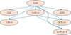 |
Fig. 11 Hierarchy of model categories examined by RTModel. 1L1S means single-lens-single-source, 1L2S is single-lens-binary-source, 2L1S is binary-lens-single-source. “+p” indicates the presence of parallax, “+x” is xallarap, and “+o” is lens orbital motion. The arrows go from lower-dimensionality models to higher-dimensionality models that include them as special cases (nested models). |
χ2 thresholds at 5σ required to validate a test hypothesis with m additional parameters with respect to a null hypothesis.
9 WFIRST data challenge
RTModel has been active since 2013 with hundreds of microlensing events analyzed in real time and visible on a public repository, as noted in the introduction to this paper. A similar number has been analyzed offline within particular projects. Specific modules of RTModel have naturally evolved over these ten years to enhance the effectiveness on all classes of microlensing events.
An ideal opportunity to assess the effectiveness of RTModel approach came in 2018 by the WFIRST data challenge7. The goal of this competition was to stimulate new ideas for the analysis of massive microlensing data as expected from the future WFIRST (now Roman) mission8. This mission will make six continuous surveys of several fields of the Galactic bulge with a duration of about two months each (Penny et al. 2019) and a cadence of 15 minutes. About 30 thousand microlensing events should be detected, with more than 1000 planets to be discovered in a wide range of masses, from Jupiters down to Mars-mass planets. This survey will complement Kepler statistics (Borucki et al. 2010) in the outer regions of planetary systems beyond the so-called snow line Burn et al. (2021); Gaudi et al. (2021).
The analysis of several thousand microlensing events requires a software that is fast enough to ingest such a copious data flow and effective enough to discriminate true planets from contaminants and provide at least reasonable preliminary models that provide a good basis for further investigation. In the WFIRST data challenge, 293 light curves were simulated with the predicted cadence, the expected scatter in the photometry and all other survey specifications. These light curves included single-lens microlensing events, binary-lens, planetary-lens microlensing, and some known contaminants, such as cataclismic variables. The participant teams were asked to provide an assessment for each light curve and a model.
RTModel took part in the data challenge proposing the only existing completely automatic algorithm running without any human intervention from the data preparation to the final assessment for each light curve. The success rate of our automatic interpretation and classification at that time was very encouraging and comparable to other platforms involving some human intervention or vetting at some level.
In the five years after that challenge, RTModel has continued its evolution. The version we are describing here and that is being released to the public has some important differences compared to the 2019 data challenge version. Nevertheless, we can still repeat the challenge using the same 293 simulated light curves and assess the performance of the current version on this well-established independent benchmark.
The success rates for single-lens, binary, and planetary microlensing events are summarized in Table 2 and visualized through pie charts in Fig. 12. The success rate is 98% for single-lens events, 74% for binary lenses with a mass ratio q > 0.03, and 77% for planetary lenses with q < 0.03. These numbers might look relatively low for a modeling platform that promises efficient modeling for massive data flows, but here we propose a closer look at the “failures” before making our considerations.
Close/wide. In this column, we collect cases where the data were simulated with a certain binary model and RTModel found a model with the same parameters except that the separation was the dual under the transformation s → 1/s (Griest & Safizadeh 1998; Dominik 1999; Bozza 2000; An 2005). In principle, we would like to have both solutions in the final selection of proposed models, but RTModel did not find or discarded one of the two in its selection process. The impact of such a loss is, however, marginal, since the planet is recovered anyway and detailed modeling after the preliminary search may also check the dual solution just to be sure that all possible models have been taken in consideration before the finalization of the analysis. Thus, depending on the analysis protocol, these events could be even included in the successful cases, raising the success rate to 80% for binary and 91% for planetary events.
Undetected. Some anomalies in the simulated data are so subtle that were overlooked by RTModel. When the anomaly is at the noise level, a fully automatic platform may have a hard time in detecting and/or modeling such anomalies. Depending on the analysis protocol that is adopted, such events may even pass undetected before they are sent to RTModel. So, if we remove them from our count, the success rate reaches 100% for single-lens, 84% for binary, and 94% for planetary events.
Different models. These are the cases in which RTModel found a completely different model with respect to the simulated event. More investigation is needed to understand why the correct model was missed. In the case of planetary events, it might happen that the light curve can be also perfectly fit by a binary-lens model, as it is well known from several documented cases (Han & Gaudi 2008; Han 2009). For binary-lens events, we had some problems in recovering events with strong orbital motion. One reason may come from the fact that the simulated events were built with two-parameters orbital motion, which is notoriously unphysical (Bozza et al. 2021; Ma et al. 2022). In such cases, these light curves should be rather removed from the challenge. On the other hand, we can reasonably expect that strong orbital motion cannot be recovered by the perturbative approach pursued by RTModel in its default configuration. For events in which higher order effects are too strong, RTModel should be set to include parallax and/or orbital motion from the very beginning of the search.
All events for which the model was not perfectly found by RTModel are collected in Table 3. Apart from the well-known degeneracies discussed before, many events (in particular binaries) suffer from a different treatment of orbital motion. With a success rate ranging from 74 to 94%, depending on the metrics we prefer to adopt, we consider the results obtained with the default settings of RTModel extremely encouraging. By tuning the options in some specific way, most of the missed models can be promptly recovered with little more investment in computational time. Of course, there are still good margins for improvement for RTModel in some particular limits, as discussed above. This is one of the commitments that we take for future versions.
Successes and failures of RTModel on the 2018 WFIRST data challenge using the default settings.
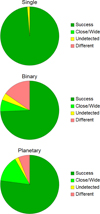 |
Fig. 12 Pie charts for the results obtained by running the public version of RTModel with the default settings on the 2019 WFIRST data challenge (see Table 2). |
Events in the data challenge for which RTModel does not return the correct model with the default options.
10 Conclusions
One of the things that makes microlensing so exciting is in the difficulties of modeling. The way a combination of caustics and particular source trajectories may create spectacular brightening and dimming episodes is fascinating. Furthermore, coding what human intuition sees in these patterns into a general software that is able to deal with all possible realistic cases remains a formidable challenge. Grid searches on the vast microlensing parameter space requires expensive clusters and may be unscalable to large data flows as those expected from the Roman mission. It is thus important to invest in alternative algorithms that drive the fit after a preliminary analysis of the features appearing in the data.
This is exactly the philosophy of RTModel, deployed in 2013 to model microlensing events in real time with a fast Levenberg-Marquardt algorithm from a set of templates covering all possible categories of microlensing light curves. These templates are matched to features recognized in the light curve and provide efficient initial conditions for fitting. The bumper mechanism acting at minima previously found broadens the exploration of the parameter space. Finally, we should not forget that VBBinaryLensing was created within the original RTModel project and was then made public as a independently appreciated spin-off. RTModel also proposes an automatic classification of the light curve based on statistical thresholds to be applied to the χ2 obtained with different model categories. This can be particularly useful when dealing with large number of light curves that cannot be visually inspected one by one.
As we have seen after the WFIRST data challenge, there are margins for improvement for RTModel, in particular for low-signal anomalies and for long binary events that cannot be recovered as perturbations of static models. Alternative parameterizations can also be useful in particular cases. Future developments may aim at incorporating new algorithms in the general architecture of the software recovering such “tricky” events and approaching a 100% efficiency. In this respect, more focused simulations may be helpful to single out those situations where the general algorithm is less efficient.
The modular structure of RTModel makes it very flexible to further additions or replacements of individual steps in the modeling run. The same template library can be customized or extended by users to improve the efficiency on specific situations. Future extensions that will be reasonably achieved in the mid- or long-term include astrometric microlensing, Markov chain exploration, Bayesian analysis with interface to Galactic models, triple and/or multiple lenses, and/or binary sources.
In addition to these functionalities, the publication of our algorithms will allow for future microlensing pipelines to benefit from the long experience gained by RTModel and promote the design of even more efficient platforms. Indeed, we believe that RTModel will stand as a reference platform in microlensing for general-purpose modeling for many years going forward.
Acknowledgements
We thank Greg Olmschenck for a revision and refinement of the installation of the RTModel package to make it as cross-platform as possible. We also thank Etienne Bachelet and Fran Bartolic for help and advice spreading from VBBinaryLensing to RTModel. We acknowledge financial support from PRIN2022 CUP D53D23002590006.
Appendix A Template library for initial conditions
As explained in Sec. 4.4, initial conditions for binary-lens models are set by matching of peaks in the data to peaks in the template light curves in a library. Here we list all templates with their parameters in the following table
Parameters of the templates used to set initial conditions.
References
- Alcock, C., Allsman, R. A., Alves, D., et al. 1999, ApJ, 518, 44 [NASA ADS] [CrossRef] [Google Scholar]
- An, J. H. 2005, MNRAS, 356, 1409 [Google Scholar]
- Bachelet, E., Norbury, M., Bozza, V., & Street, R. 2017, AJ, 154, 203 [NASA ADS] [CrossRef] [Google Scholar]
- Bachelet, E., Bozza, V., Han, C., et al. 2019, ApJ, 870, 11 [NASA ADS] [CrossRef] [Google Scholar]
- Beaulieu, J. P., Bennett, D. P., Fouqué, P., et al. 2006, Nature, 439, 437 [NASA ADS] [CrossRef] [Google Scholar]
- Bennett, D. P. 2010, ApJ, 716, 1408 [NASA ADS] [CrossRef] [Google Scholar]
- Bennett, D. P., & Rhie, S. H. 1996, ApJ, 472, 660 [NASA ADS] [CrossRef] [Google Scholar]
- Borucki, W. J., Koch, D., Basri, G., et al. 2010, Science, 327, 977 [Google Scholar]
- Bozza, V. 1999, A&A, 348, 311 [NASA ADS] [Google Scholar]
- Bozza, V. 2000, A&A, 355, 423 [NASA ADS] [Google Scholar]
- Bozza, V. 2010, MNRAS, 408, 2188 [NASA ADS] [CrossRef] [Google Scholar]
- Bozza, V., Dominik, M., Rattenbury, N. J., et al. 2012, MNRAS, 424, 902 [Google Scholar]
- Bozza, V., Shvartzvald, Y., Udalski, A., et al. 2016, ApJ, 820, 79 [NASA ADS] [CrossRef] [Google Scholar]
- Bozza, V., Bachelet, E., Bartolić, F., et al. 2018, MNRAS, 479, 5157 [Google Scholar]
- Bozza, V., Khalouei, E., & Bachelet, E. 2021, MNRAS, 505, 126 [NASA ADS] [CrossRef] [Google Scholar]
- Burn, R., Schlecker, M., Mordasini, C., et al. 2021, A&A, 656, A72 [NASA ADS] [CrossRef] [EDP Sciences] [Google Scholar]
- Dominik, M. 1995, A&AS, 109, 597 [NASA ADS] [Google Scholar]
- Dominik, M. 1998, A&A, 333, L79 [NASA ADS] [Google Scholar]
- Dominik, M. 1999, A&A, 349, 108 [NASA ADS] [Google Scholar]
- Dominik, M., Rattenbury, N. J., Allan, A., et al. 2007, MNRAS, 380, 792 [NASA ADS] [CrossRef] [Google Scholar]
- Dominik, M., Horne, K., Allan, A., et al. 2008, Astron. Nachr., 329, 248 [NASA ADS] [CrossRef] [Google Scholar]
- Dominik, M., Bachelet, E., Bozza, V., et al. 2019, MNRAS, 484, 5608 [CrossRef] [Google Scholar]
- Erdl, H., & Schneider, P. 1993, A&A, 268, 453 [NASA ADS] [Google Scholar]
- Fukui, A., Suzuki, D., Koshimoto, N., et al. 2019, AJ, 158, 206 [NASA ADS] [CrossRef] [Google Scholar]
- Gaudi, B. S. 2012, ARA&A, 50, 411 [Google Scholar]
- Gaudi, B. S., & Gould, A. 1997, ApJ, 486, 85 [Google Scholar]
- Gaudi, B. S., Meyer, M., & Christiansen, J. 2021, in ExoFrontiers; Big Questions in Exoplanetary Science, ed. N. Madhusudhan (Bristol: IOP Publishing), 2 [Google Scholar]
- Glover, F. 1989, ORSA J. Comput., 1, 190 [CrossRef] [Google Scholar]
- Glover, F. 1990, ORSA J. Comput., 2, 4 [CrossRef] [Google Scholar]
- Gould, A. 1992, ApJ, 392, 442 [Google Scholar]
- Gould, A., & Gaucherel, C. 1997, ApJ, 477, 580 [Google Scholar]
- Gould, A., & Loeb, A. 1992, ApJ, 396, 104 [Google Scholar]
- Griest, K., & Safizadeh, N. 1998, ApJ, 500, 37 [Google Scholar]
- Han, C. 2006, ApJ, 638, 1080 [Google Scholar]
- Han, C. 2009, ApJ, 691, L9 [Google Scholar]
- Han, C., & Gaudi, B. S. 2008, ApJ, 689, 53 [CrossRef] [Google Scholar]
- Han, C., Udalski, A., Jung, Y. K., et al. 2024, A&A, 685, A16 [NASA ADS] [CrossRef] [EDP Sciences] [Google Scholar]
- Henderson, C. B., Poleski, R., Penny, M., et al. 2016, PASP, 128, 124401 [NASA ADS] [CrossRef] [Google Scholar]
- Herald, A., Udalski, A., Bozza, V., et al. 2022, A&A, 663, A100 [NASA ADS] [CrossRef] [EDP Sciences] [Google Scholar]
- Hundertmark, M., Street, R. A., Tsapras, Y., et al. 2018, A&A, 609, A55 [NASA ADS] [CrossRef] [EDP Sciences] [Google Scholar]
- Koshimoto, N., Sumi, T., Bennett, D. P., et al. 2023, AJ, 166, 107 [NASA ADS] [CrossRef] [Google Scholar]
- Levenberg, K. 1944, Quarterly Appl. Math., 2, 164 [Google Scholar]
- Liebig, C., D’Ago, G., Bozza, V., & Dominik, M. 2015, MNRAS, 450, 1565 [NASA ADS] [CrossRef] [Google Scholar]
- Ma, X., Zhu, W., & Yang, H. 2022, MNRAS, 513, 5088 [NASA ADS] [CrossRef] [Google Scholar]
- Mao, S. 2012, Res. Astron. Astrophys., 12, 947 [Google Scholar]
- Mao, S., & Di Stefano, R. 1995, ApJ, 440, 22 [NASA ADS] [CrossRef] [Google Scholar]
- Mao, S., & Paczynski, B. 1991, ApJ, 374, L37 [NASA ADS] [CrossRef] [Google Scholar]
- Marquardt, D. 1963, SIAM J. Appl. Math., 11, 431 [CrossRef] [Google Scholar]
- Mroz, P., & Poleski, R. 2024, Exoplanet Occurrence Rates from Microlensing Surveys, in Deeg, H.J., Belmonte, J.A. (eds) Handbook of Exoplanets (Springer) [Google Scholar]
- Paczynski, B. 1986, ApJ, 304, 1 [NASA ADS] [CrossRef] [Google Scholar]
- Penny, M. T., Gaudi, B. S., Kerins, E., et al. 2019, ApJS, 241, 3 [CrossRef] [Google Scholar]
- Poleski, R., & Yee, J. C. 2019, Astron. Comput., 26, 35 [NASA ADS] [CrossRef] [Google Scholar]
- Ranc, C., & Cassan, A. 2018, Astrophysics Source Code Library [record ascl:1811.012] [Google Scholar]
- Rattenbury, N. J., Bennett, D. P., Sumi, T., et al. 2015, MNRAS, 454, 946 [NASA ADS] [CrossRef] [Google Scholar]
- Rota, P., Hirao, Y., Bozza, V., et al. 2021, AJ, 162, 59 [NASA ADS] [CrossRef] [Google Scholar]
- Schneider, P., & Weiss, A. 1986, A&A, 164, 237 [NASA ADS] [Google Scholar]
- Skowron, J., & Gould, A. 2012, arXiv e-prints [arXiv:1203.1034] [Google Scholar]
- Street, R. A., Bachelet, E., Tsapras, Y., et al. 2019, AJ, 157, 215 [NASA ADS] [CrossRef] [Google Scholar]
- Sumi, T., Koshimoto, N., Bennett, D. P., et al. 2023, AJ, 166, 108 [NASA ADS] [CrossRef] [Google Scholar]
- Tsapras, Y. 2018, Geosciences, 8, 365 [NASA ADS] [CrossRef] [Google Scholar]
- Tsapras, Y., Choi, J. Y., Street, R. A., et al. 2014, ApJ, 782, 48 [NASA ADS] [CrossRef] [Google Scholar]
- Tsapras, Y., Cassan, A., Ranc, C., et al. 2019, MNRAS, 487, 4603 [NASA ADS] [CrossRef] [Google Scholar]
- Udalski, A., Han, C., Bozza, V., et al. 2018, ApJ, 853, 70 [NASA ADS] [CrossRef] [Google Scholar]
- Yee, J. C., Anderson, J., Akeson, R., et al. 2018, arXiv e-prints [arXiv:1803.07921] [Google Scholar]
- Zhang, K., & Gaudi, B. S. 2022, ApJ, 936, L22 [NASA ADS] [CrossRef] [Google Scholar]
All Tables
χ2 thresholds at 5σ required to validate a test hypothesis with m additional parameters with respect to a null hypothesis.
Successes and failures of RTModel on the 2018 WFIRST data challenge using the default settings.
Events in the data challenge for which RTModel does not return the correct model with the default options.
All Figures
|
Fig. 1 Flow chart of RTModel with the different modules in green and the data and/or products in blue ovals. The orange box highlights the modules that are called repeatedly for each model category with their respective products. |
| In the text | |
|
Fig. 2 Assessment of scatter in the photometry. The green point is one-sigma above extrapolation from the two preceding points and half-sigma from the extrapolation of the two following points. |
| In the text | |
|
Fig. 3 Identification of an outlier: if the extrapolations from the preceding and following points agree, a threshold is set for the residual of the current point. Beyond this threshold, the point is removed as outlier. |
| In the text | |
|
Fig. 4 Re-binning at work on a simulated event. Points from the original data untouched by re-binning are in green. Original points replaced by their re-binned versions with neighbors are in blue, new points resulting from re-binning are in yellow. |
| In the text | |
|
Fig. 5 Spline model for a simulated dataset. Concave sections are also highlighted with different colors. |
| In the text | |
|
Fig. 6 Example of template matching to some simulated data using template # 47. |
| In the text | |
|
Fig. 7 Determination of initial conditions for planetary fits in the wide configuration. The blue caustic comes with the choice s = s+ and the green caustic with s = s−. |
| In the text | |
|
Fig. 8 Determination of initial conditions for planetary fits in the close configuration. The blue caustic comes with the choice α = α+ and the green caustic with α = α−. |
| In the text | |
|
Fig. 9 Bumper mechanism to jump out of local minima. The fit coming from x−1 ends in x, within the covariance ellipsoid of the previously found minimum x0. It is then bumped to |
| In the text | |
|
Fig. 10 Fit track obtained on some simulated data projected to the plane (ln s, ln q) in a binary-lens fit. We see that the first fit (red track) ended at a local minimum with high χ2. Then, repeating the fit with the bumper mechanism leads to a different region with a much lower χ2, where some more minima are found. |
| In the text | |
|
Fig. 11 Hierarchy of model categories examined by RTModel. 1L1S means single-lens-single-source, 1L2S is single-lens-binary-source, 2L1S is binary-lens-single-source. “+p” indicates the presence of parallax, “+x” is xallarap, and “+o” is lens orbital motion. The arrows go from lower-dimensionality models to higher-dimensionality models that include them as special cases (nested models). |
| In the text | |
|
Fig. 12 Pie charts for the results obtained by running the public version of RTModel with the default settings on the 2019 WFIRST data challenge (see Table 2). |
| In the text | |
Current usage metrics show cumulative count of Article Views (full-text article views including HTML views, PDF and ePub downloads, according to the available data) and Abstracts Views on Vision4Press platform.
Data correspond to usage on the plateform after 2015. The current usage metrics is available 48-96 hours after online publication and is updated daily on week days.
Initial download of the metrics may take a while.