| Issue |
A&A
Volume 688, August 2024
|
|
|---|---|---|
| Article Number | A16 | |
| Number of page(s) | 12 | |
| Section | Interstellar and circumstellar matter | |
| DOI | https://doi.org/10.1051/0004-6361/202450188 | |
| Published online | 29 July 2024 | |
Multiline study of the radial extent of SiO, CS, and SiS in asymptotic giant branch envelopes★
1
Instituto de Física Fundamental,
CSIC, C/ Serrano 123,
28006
Madrid,
Spain
e-mail: This email address is being protected from spambots. You need JavaScript enabled to view it.
; This email address is being protected from spambots. You need JavaScript enabled to view it.
2
Centro de Astrobiología (CSIC/INTA),
Ctra. de Ajalvir km. 4, Torrejón de Ardoz,
28850
Madrid,
Spain
3
Observatorio Astronómico Nacional (IGN),
Alfonso XII 3,
28014
Madrid,
Spain
Received:
29
March
2024
Accepted:
29
May
2024
Abstract
Circumstellar envelopes around asymptotic giant branch (AGB) stars contain a rich diversity of molecules, whose spatial distribution is regulated by different chemical and physical processes. In the outer circumstellar layers, all molecules are efficiently destroyed due to interactions with interstellar ultraviolet photons. Here we aim to carry out a coherent and uniform characterization of the radial extent of three molecules (SiO, CS, and SiS) in envelopes around O- and C-rich AGB stars, and to study their dependence on mass-loss rate. To this end, we observed a reduced sample of seven M-type and seven C-type AGB envelopes in multiple lines of SiO, CS, and SiS with the Yebes 40 m and IRAM 30 m telescopes. The selected sources cover a wide range of mass-loss rates, from ~10−7 M⊙ yr−1 to a few times 10−5 M⊙ yr−1, and the observed lines cover a wide range of upper-level energies, from 2 K to 130 K. We carried out excitation and radiative transfer calculations over a wide parameter space in order to characterize the abundance and radial extent of each molecule. A χ2 analysis indicates that the abundance is usually well constrained while the radial extent is in some cases more difficult to constrain. Our results indicate that the radial extent of the molecules considered here increases with increasing envelope density, in agreement with previous observational findings. At high envelope densities of Ṁ/υ∞ > 10−6 M⊙ yr−1 km−1 s, SiO, CS, and SiS show a similar radial extent, while at low envelope densities of Ṁ/υ∞ < 10−7 M⊙ yr−1 km−1 s, differences in radial extent appear among the three molecules, in agreement with theoretical expectations based on destruction due to photodissociation. At low envelope densities, we find a sequence of increasing radial extent, SiS → CS → SiO. We also find a tentative dependence of the radial extent on the chemical type (O- or C-rich) of the star for SiO and CS. Interferometric observations and further investigation of the photodissociation of SiO, CS, and SiS should provide clarification of the situation in regards to the relative photodissociation radii of SiO, CS, and SiS in AGB envelopes and their dependence on envelope density and C/O ratio.
Key words: astrochemistry / molecular processes / stars: AGB and post-AGB / radio lines: stars
Based on observations carried out with the IRAM 30 m and Yebes 40 m telescopes. IRAM is supported by INSU/CNRS (France), MPG (Germany) and IGN (Spain). The Yebes 40 m telescope at Yebes Observatory is operated by the Spanish Geographic Institute (IGN, Ministerio de Transportes, Movilidad y Agenda Urbana).
© The Authors 2024
 Open Access article, published by EDP Sciences, under the terms of the Creative Commons Attribution License (https://creativecommons.org/licenses/by/4.0), which permits unrestricted use, distribution, and reproduction in any medium, provided the original work is properly cited.
This article is published in open access under the Subscribe to Open model. This email address is being protected from spambots. You need JavaScript enabled to view it. to support open access publication.
1 Introduction
The circumstellar envelopes (CSEs) of asymptotic giant branch (AGB) stars are made of molecules and dust. Some molecules are formed in the warm and dense inner regions – where abundances are thought to be largely controlled by chemical equilibrium (Tsuji 1973; Agúndez et al. 2020) – and are then injected into the expanding envelope. These molecules, some of which contain refractory elements, are simple and stable species, such as CO, H2O, HCN, C2H2, H2S, CS, SiO, SiS, SiC2, NaCl, and AlCl. Other species, such as radicals and, in the case of C-rich objects, long carbon chains are formed in the outer layers under the action of photochemistry, which is driven by the penetration of interstellar ultraviolet (UV) photons.
Molecular abundances are subject to variation as the gas travels away from the star due to interactions with dust grains, gas-phase chemistry, and photodissociation, which eventually destroys all molecules in the tenuous and translucent outer layers. Molecular hydrogen and CO are the two molecules that survive out to larger distances, because their high abundances and the fact that they are photodissociated in lines mean that they self-shield against interstellar UV photons (Morris & Jura 1983). All other molecules extend out to shorter distances from the star.
In order to gain a firm understanding of circumstellar chemistry, it is important to constrain the radial extent of the different molecules. The spatial distribution of CO has been constrained observationally by mapping low-energy rotational lines (Castro-Carrizo et al. 2010; Ramstedt et al. 2020), and theoretically by modeling its photodissociation (Groenewegen et al. 2017; Saberi et al. 2019; Groenewegen & Saberi 2021). For other molecules, the radial extent has also been constrained observa-tionally by modeling multiple rotational lines, as in the cases of SiO (González Delgado et al. 2003; Schöier et al. 2006a), SiS and CS (Schöier et al. 2007; Danilovich et al. 2018), and HCN (Schöier et al. 2013). For some of these molecules, there are also constraints on their abundance distribution in selected objects from large-scale mapping of selected rotational lines (Velilla-Prieto et al. 2019; Danilovich et al. 2019).
To determine accurate molecular abundances in AGB envelopes from single-dish observations, it is of paramount importance to know how far each molecule extends, especially if only a few lines are available. This was the case in our previous studies, in which we determined the abundances of the molecules SiC2, SiO, CS, and SiS in a large sample of AGB envelopes using just a few rotational lines (Massalkhi et al. 2018, 2019, 2020). Here, we aim to use multiple rotational lines to carry out a systematic and coherent determination of the radial extent of SiO, CS, and SiS in a reduced sample of O-rich and C-rich AGB envelopes spanning a wide range of mass-loss rates. This valuable information can be used to derive accurate abundances for these three molecules in circumstellar envelopes around other AGB stars. In addition, our comparative study allows us to shed light on the different behavior of each molecule when faced with photodissociation. We present the observations carried out in Sect. 2, describe the adopted model in Sect. 3, discuss the obtained results in Sect. 4, and present our conclusions in Sect. 5.
Sample of AGB envelopes and associated parameters.
2 Observations
We selected a sample of 14 AGB envelopes: half of them of M-type (oxygen-rich) from the sample of Massalkhi et al. (2020) and the other half of C-type (carbon-rich) from Massalkhi et al. (2019). The sources, which are listed in Table 1, were chosen to cover a wide range of mass-loss rates, from 10−7 M⊙ yr−1 to a few times 10−5 M⊙ yr−1. We used the IRAM 30 m telescope in several sessions from March 2019 to June 2020 and the Yebes 40 m telescope from December 2019 to September 2020. In the case of IRC+10216, the Yebes 40 m observations correspond to the high-sensitivity spectral survey described in Pardo et al. (2022).
The IRAM 30 m observations consist of specific frequency setups across the different available bands. The covered frequency ranges were 81.3–89.1 GHz and 96.9–104.7 GHz (3 mm band), 237.8–245.6 GHz and 253.4–261.2 GHz (1.3 mm band), and 287.1–294.9 GHz and 302.7–310.5 GHz (0.9 mm band). We used the E090, E230, and E330 receivers in dual side band, with image rejections of >10 dB, connected to a FFTS providing a spectral resolution of 195 kHz, which for our target lines corresponds to velocity resolutions in the range of 0.2–0.7 km s−1. We used the wobbler-switching observing mode, with a throw of 180″ in azimuth. The focus of the telescope was regularly checked on a planet. The half power beam width (HPBW) of the 30 m telescope ranges between 28″ at 87 GHz and 8″ at 309 GHz. The pointing was systematically checked every 1 h on a nearby quasar, with errors within 2–3″. The intensity scale at the 30 m telescope is the antenna temperature corrected for atmospheric absorption and for antenna ohmic and spillover losses,  , for which we estimate a calibration error of 10% at 3 mm, 20% at 2 mm, and 30% in the 1.3 and 0.9 mm bands. The
  scale is converted to Tmb (main beam brightness temperature) by dividing by Beff/Feff, where Beff = 0.871 exp[−(v( GHz)/359)2] and Feff takes values of 0.95, 0.93, 0.92, and 0.82 at 3, 2, 1.3, and 0.9 mm, respectively.
The Yebes 40 m observations consisted in a full scan of the Q band, from 31 to 50 GHz. We used a 7 mm receiver connected to a fast Fourier transform spectrometer (FFTS), which provides an instantaneous coverage of the whole Q band in horizontal and vertical polarizations with a spectral resolution of 38 kHz (see Tercero et al. 2021). Spectra were later smoothed to a spectral resolution of 191 kHz, which corresponds to velocity resolutions in the range 1.1–1.8 km s−1 across the Q band. The observations were carried out in the position-switching mode, with the off position shifted by 300″ in azimuth with respect to the source position. The HPBW ranges between 35″ at 50 GHz and 57″ at 31 GHz. Pointing corrections were obtained by observing SiO masers and quasars and were always within 2–3″. The intensity scale at the 40 m telescope is  , for which we estimate a calibration error of 10%. We converted
  to Tmb by dividing by Beff/Feff, where Beff = 0.797 exp[–(v (GHz)/71.1)2] and Feff = 0.97.
The Yebes 40 m and IRAM 30 m observations allowed us to cover multiple rotational lines of SiO, CS, and SiS with a wide range of upper-level energies (see Table 2). The observed lines are shown in Fig. A.1. The line profiles were fitted using the SHELL method implemented in the program CLASS within the GILDAS software (Pety 2005)1. The line parameters are given in Table A.1. Some of the targeted lines were not detected in all sources. In some cases, the line was detected but the intensity was suspected to be erroneous, which was very likely due to problems in the calibration or the pointing, especially for those lines lying at high frequencies. The nondetections and the problematic observations have been omitted in Fig. A.1 and Table A.1. The sources IK Tau and IRC +10216 were not observed with the IRAM 30 m telescope because there are extensive data available from Velilla-Prieto et al. (2017) and Agúndez et al. (2012). We did not observe the 2 mm band because we have IRAM 30 m data from previous studies (Massalkhi et al. 2018, 2019, 2020).
We also used the IRAM 30 m telescope in May and September 2022 to observe the CO J = 1–0 and J = 2–1 lines toward CRL 190 and IRC +30374. These data are needed to model the gaseous envelope, as described in Sect. 3.2, but are not available in the literature. The velocity-integrated line intensities are given in TableA.3.
Lines observed in this study.
3 Envelope model
Our main objective is to constrain the radial extent of SiO, CS, and SiS in the observed sources. We therefore built a model of each of the sources and performed excitation and radiative transfer calculations to produce synthetic lines for comparison with the observed lines. To describe the observed objects, we consider an idealized model consisting of a spherical envelope of gas and dust expanding around a central AGB star, which is characterized by a luminosity, L⋆, and an effective temperature, T⋆. Dust is assumed to be present only beyond the condensation radius, rc, with a constant gas-to-dust mass ratio, Ψ. The envelope is characterized by a constant mass-loss rate, Ṁ, and a radial expansion velocity, υexp, which is assumed to be uniform and equal to υ0 between the star surface and the dust condensation radius, while outside rc it can be expressed as a function of radius, r, as (Höfner & Olofsson 2018)
 (1)
(1)
where υ∞ is the terminal expansion velocity and we assume υ0 = υ∞/4 and β =1 based on observational constraints (Decin et al. 2010). The volume density of gas particles, ng, is given by the law of conservation of mass as
 (2)
(2)
where  is the average mass of gas particles, assumed to be 2.3 amu after considering H2, He, and CO. As we are mainly interested in the outer layers, for simplicity we assume υexp to be equal to υ∞ in Eq. (2). The gas kinetic temperature, Tg, is assumed to be given by the expression
 (3)
(3)
where the exponent δ is determined from a fit to multiple CO lines (see Sect. 3.2) and Tg is not allowed to decrease below 10 K. Although Eq. (3) does not account for the underlying processes of heating and cooling of the gas, it provides a reasonable first-order approximation to the radial temperature profile (e.g., De Beck et al. 2010). The stellar radius, R⋆, is set by the luminosity and effective temperature, as
 (4)
(4)
where σSB is the Stefan-Boltzmann constant. The dust temperature is calculated as a function of radius from a fit to the spectral energy distribution (SED) of the envelope (see Sect. 3.1).
The parameters needed to describe the envelope model for each of the sources are given in Table 1. The distances, D, were mainly taken from the Gaia Data Release 3 (DR3; Gaia Collaboration 2023). We note that the adopted distances are within 20% of the values recommended by Andriantsaralaza et al. (2022), except for GX Mon, for which these authors recommend a much larger distance of 1430 pc based on the period–luminosity relation. The systemic velocities, Vsys, in the Local Standard of Rest (LSR) frame and the terminal expansion velocities, υ∞, were determined for the C-rich stars by Massalkhi et al. (2018) and for the O-rich stars by Massalkhi et al. (2020) from various intense lines. The stellar effective temperatures, T⋆, are from different literature sources. The remaining parameters in Table 1 were determined in this study. On the one hand, the stellar luminosity, L⋆, the optical depth at 10 µm, τ10, the dust condensation radius, rc, the dust temperature at the dust condensation radius, Td(rc), and the gas-to-dust mass ratio, Ψ, are determined from a fit to the SED (see details in Sect. 3.1). On the other hand, the mass-loss rate, Ṁ, and the exponent δ in the gas kinetic temperature radial profile in Eq. (3), are determined from a fit to multiple CO lines, as described in Sect. 3.2.
The fitting strategy used to reproduce the SED and the CO lines (and also subsequently the lines of SiO, CS, and SiS) is based on the minimization of the parameter χ2, which is defined as
![Mathematical equation: ${\chi ^2} = \sum\limits_{i = 1}^N {{{\left[ {{{\left( {{I_{{\rm{calc }}}} - {I_{{\rm{obs}}}}} \right)} \over \sigma }} \right]}^2}} ,$](/articles/aa/full_html/2024/08/aa50188-24/aa50188-24-eq10.png) (5)
(5)
where the sum extends over N independent observations, ƒcalc and Iobs are the calculated and observed intensities, and σ are the uncertainties on Iobs. We run many models (typically between 100 and 1000) in which we vary the values of the different free input parameters and take the best-fit model to be that which results in the minimum value of χ2,  . To evaluate the goodness of the fit, we use the reduced χ2, defined as
 (6)
(6)
where p is the number of free input parameters. Typically, a value of  indicates a good-quality fit. The methodology provides best-fit values for the p adjustable parameters and uncertainties for them, given as the standard deviation σ. For p = 1, the 1 σ level (68% confidence) is given by χ2 + 1.00, while for p= 2 (which is usually the case here) the 1σ level is given by χ2 +2.30.
3.1 Model of the dusty envelope: Fit to SED
In order to calculate the SED of each envelope, we used the code DUSTY V2 (Ivezić & Elitzur 1997)2, which solves the continuum radiative transfer including light scattering in a spherically symmetric envelope, where dust is present from an inner condensation radius, rc. For simplicity, we assume that grains are spherical with a single size (radius of 0.1 µm) and adopt the optical constants of warm silicate (Suh 1999) for O-rich stars and of amorphous carbon (Suh 2000) for C-rich stars.
The adjustable parameters in the χ2 analysis are the dust temperature at the condensation radius, Td(rc), and the dust optical depth at a reference wavelength of 10 µm, τ10. The approach used here is similar to that employed in previous studies by F. L. Schöier and colleagues (e.g., Schöier et al. 2002, 2006a). The observed SED consists of photometric fluxes measured mostly by space telescopes at infrared wavelengths, which are obtained from the VizieR database (Ochsenbein et al. 2000)3. The fluxes collected for the 14 stars studied here are given in Table A.2. Since the observed fluxes at different wavelengths differ by orders of magnitude, we use the decimal logarithm of the observed flux as Iobs in Eq. (5). The uncertainties on the observed fluxes are not determined in a consistent way in the different catalogs and therefore we adopt a uniform uncertainty of 20% for all observed fluxes.
Figure 1 shows the results of the SED analysis for one O-rich envelope, IK Tau, and one C-rich envelope, IRC + 10216. The left panels show the SED of the best-fit model superimposed on the observed fluxes, while the right panels show the χ2 parameter as a function of the two adjustable parameters. The results of the SED analysis for the remaining 12 envelopes are shown in Fig. A.2. The observed SEDs are reasonably well fitted for all sources, with  values systematically below one. The calculated SEDs of the O-rich sources show a prominent emission band around 10 µm that is due to silicate, while in the case of the C-rich sources the amorphous carbon provides a smooth continuum in the calculated SED. We note that while the optical depth at 10 µm, τ10, is constrained to relatively narrow ranges, the dust temperature at the condensation radius, Td(rc), is poorly constrained in many of the envelopes, in particular in those with low mass-loss rates, such as R Leo, R Cas, Y CVn, and R Lep (see Fig. A.2). The best-fit values of the parameters Td(rc) and τ10 are given in Table 1. The values of τ10 obtained here are similar to those reported by Schöier et al. (2013) – in most cases they are within a factor of two. However, in the case of Td(rc) there are differences of as large as 500 K between our values and those of Schöier et al. (2013), which illustrates the larger error in the determination of this parameter.
In addition to Td(rc) and τ10, the dust radiative transfer calculations provide some parameters that are needed to describe the envelope and perform the excitation and radiative transfer calculations of molecules. These parameters are the dust condensation radius, rc, the bolometric luminosity, L⋆, and the gas-to-dust mass ratio, Ψ, all of which are given in Table 1. The parameter Ψ is computed from the column density of dust – which can be evaluated using τ10 and the optical constants of dust – and the column density of gas beyond the dust condensation radius – which is set by the gas mass-loss rate (determined by modeling the CO lines; see Sect. 3.2). In addition, the output of the DUSTY V2 code provides the dust temperature as a function of radius.
3.2 Model of the gaseous envelope: Fit to CO
To have a consistent model for each studied source, rather than taking mass-loss rates from the literature, we determined them by modeling multiple CO lines. The model, which is described at the beginning of Sect. 3, consists of a spherical envelope around an AGB star where various physical quantities may experience variations with radius. More specifically, the expansion velocity, gas volume density, and gas kinetic temperature are given by Eqs. (1)–(3). The microturbulence velocity is taken as 1 km s–1 throughout the envelope (see Massalkhi et al. 2018). To be consistent with the dust radiative transfer calculations described in Sect. 3.1, we assume that dust grains, with a radius of 0.1 µm and a density of 3.3 g cm–3 for silicate and 2.0 g cm–3 for amorphous carbon, are present beyond the condensation radius with a uniform gas-to-dust mass ratio and the temperature radial profile resulting from the DUSTY V2 calculations. The fractional abundance of CO with respect to H2 at the initial radius (here taken as the stellar photosphere, R⋆) is assumed to be 2.0 × 10⁻⁴ for O-rich envelopes, a value typically adopted in previous works (e.g., Olofsson et al. 2002), while in the case of C-rich envelopes we adopt a value of 6.7 × 10⁻⁴, as determined from observations of H2 toward IRC +10216 by Fonfría et al. (2022). The CO abundance fall off due to photodissociation in the outer layers is described according to the fitting formula in Groenewegen et al. (2017). This approach is mainly used for simplicity, although we note that more recent studies (Saberi et al. 2019; Groenewegen & Saberi 2021) indicate that CO sizes estimated by Groenewegen et al. (2017) could be too large by 11–60%. Observational validation of the theoretical description given by Groenewegen & Saberi (2021) would be very useful in order to shed light on this point.
The excitation and radiative transfer of CO in a circumstel-lar envelope is solved using two different methods. The first solves the excitation out of local thermodynamic equilibrium (LTE) and the radiative transfer locally using the large velocity gradient (LVG) formalism. This code has been used before; for example by Agúndez et al. (2012) and Massalkhi et al. (2018, 2019, 2020). The second is a nonLTE method based on the Monte Carlo formalism. The code uses the RATRAN algorithm (Hogerheijde & van der Tak 2000)4, which has been modified to allow for a layer-dependent number of energy levels, which is chosen depending on the local excitation conditions. This implementation facilitates the convergence when radiative pumping to vibrationally excited states is important in certain but not all circumstellar layers. We include the first 30 rotational levels within the υ = 0 and υ =1 vibrational states of CO. The highest level included (υ = 1, J = 29) has an energy of 5467 K over the ground state (υ = 0, J=0). In the Monte Carlo calculations, each shell is inspected and the levels with a marginal population are removed. The level energies are computed from the rotational constants given by Winnewiser et al. (1997) for the υ = 0 state and by Gendriesch et al. (2009) for the υ = 1 state. The line strengths are taken from Goorvitch (1994) for pure rotational transitions and from the HITRAN database (Rothman et al. 2005) for the ro-vibrational transitions. We use the rate coefficients for pure rotational transitions induced by inelastic collisions between CO and para and ortho H2 from Yang et al. (2010), where we assume the statistical ortho-to-para ratio of 3 for H2. We also include collisions between CO and He, where He is assumed to have a solar abundance of 0.17 relative to H2, using the rate coefficients from Cecchi-Pestellini et al. (2002). For ro-vibrational transitions induced by collisions, we adopt the same rate coefficients used for pure rotational transitions but decreased by a factor of 104 (typically found for similar molecules such as SiO and CS; Balança & Dayou 2017; Lique & Spielfiedel 2007).
The χ2 analysis was carried out by running CO models for each source, adopting the parameters in Table 1. The mass-loss rate, Ṁ, and the exponent, δ, describing the gas kinetic temperature radial profile according to Eq. (3), are left as adjustable parameters. Most CO line intensities were collected from the literature (see references in Table A.3), with the exception of IRC+30374 and CRL 190, for which we performed new observations (see Sect. 2). We used the velocity-integrated line intensities in the Tmb scale as ƒobs in Eq. (5). These values are given in Table A.3 for the 14 studied sources. Given the diversity of literature sources and telescopes employed, it is difficult to assign a reliable uncertainty to each individual CO observation. We therefore adopt a uniform uncertainty of 20% for all observed CO line intensities. We initially used the LVG method to explore a broad range of the parameter space [Ṁ, δ] as it is relatively fast, and later we employed the Monte Carlo method, which is more accurate although more computationally expensive, to restrict our analysis to a narrower range of the parameter space and to determine Ṁ and δ more accurately. All the results shown in this paper correspond to these latter Monte Carlo models.
Figure 2 shows the results of the CO analysis for the O-rich star IK Tau. The availability of eight CO lines allows us to tightly constrain the mass-loss rate and gas temperature exponent to Ṁ = (4.8 ± 0.7) × 10–6 M⊙ yr–1 and δ = 0.65 ± 0.06, with a  value of around one. Similar plots for the other stars of our sample (with the exception of IRC+10216, which is discussed below) are shown in Fig. A.3. In general, the mass-loss rate Ṁ is well constrained for most of the envelopes, with 1σ errors in the range of 10–30%, except for IRC+20370, for which the error is ~40%. The gas temperature exponent δ is reasonably well constrained for many of the sources, although for some of them, such as TX Cam, R Leo, Y CVn, and R Lep, the uncertainty is high, and in the case of CRL190, the parameter δ is poorly constrained. The best-fit values of Ṁ and δ are given in Table 1. The mass-loss rates derived are consistent with those derived by Schöier et al. (2013) within a factor of two. Larger differences of up to a factor of 3–4 are found for TX Cam, R Lep, LP And, and IRC +20370. In most cases, changes in Ṁ can, at least partly, be attributed to the different distances used. We note that the distances adopted here should be more accurate than those used by Schöier et al. (2013) because ours are mostly based on Gaia DR3 parallaxes (Gaia Collaboration 2023), while those of Schöier et al. are estimated from period–luminosity relationship (Whitelock et al. 1994; Groenewegen & Whitelock 1996) or from HIPPARCOS parallaxes when available.
The case of IRC+ 10216 is a special one. This is the only AGB envelope in our sample for which the mass-loss rate has been determined directly by observing H2 instead of CO (Fonfría et al. 2022). The mass-loss rate derived by these latter authors is 2.4 × 10⁻⁵ M⊙ yr–1, in agreement with the range (2–4) × 10–5 M⊙ yr–1 derived in previous studies from maps of low-J CO lines (Cernicharo et al. 2015; Guélin et al. 2018). IRC +10216 is also the only source for which we have many high-J CO lines from HIFI. If we perform a χ2 analysis with Ṁ and δ as adjustable parameters, as for the rest of the sources, the best-fit model has problems to reproduce simultaneously low-/ and high-J lines. We therefore decided to fix the mass-loss rate to the value derived by Fonfría et al. (2022) and implemented a radial gas temperature profile with three power laws to describe the inner, intermediate, and outer envelope. A similar approach was adopted by Daniel et al. (2012) to model the CO lines observed with HIFI in this source. The best-fit model is shown in Fig. 3, where the gas temperature is described by δ = 0.45 inside 1015 cm, δ = 1.55 beyond 1016 cm, and δ = 0.95 in between.
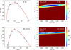 |
Fig. 1 Results from SED analysis for IK Tau and IRC +10216. The left panels show the observed fluxes in blue (see Table A.2) and the calculated SED from the best DUSTY model in red. The right panels show χ2 as a function of the dust temperature at the condensation radius, Td(rc), and the logarithm of the dust optical depth at 10 µm, log τ10. The white contours correspond to 1, 2, and 3σ levels. Similar plots for other stars are shown in Fig. A.2. |
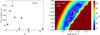 |
Fig. 2 Results from CO analysis for IK Tau. The left panel shows the observed intensities (see Table A.3) as black filled circles and the calculated ones as red empty circles. The right panel shows χ2 as a function of the logarithm of the mass-loss rate, log Ṁ, and the exponent of the gas kinetic temperature radial profile, δ. The white contours correspond to 1, 2, and 3σ levels. Similar plots for other stars are shown in Fig. A.3. |
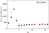 |
Fig. 3 Best-fit CO model for IRC +10216. The observed intensities (see Table A.3) are represented by black filled circles and the calculated ones by red empty circles. |
3.3 Model for SiO, CS, and SiS: Abundance and radial extent
To model the lines of SiO, CS, and SiS, we carried out excitation and radiative transfer calculations similar to those described in Sect. 3.2 for CO. The main difference is that the abundance fall off in the outer layers, which in the case of CO is described by the fitting formula of Groenewegen et al. (2017), is described now by the empirical expression
![Mathematical equation: $f(r) = {f_0}\exp \left[ { - {{\left( {{r \over {{r_e}}}} \right)}^2}} \right],$](/articles/aa/full_html/2024/08/aa50188-24/aa50188-24-eq16.png) (7)
(7)
where f is the fractional abundance relative to H2, ƒ0 is the abundance at the initial radius (taken as the stellar photosphere, R⋆), and re is the e-folding radius at which the abundance has decreased by a factor of e with respect to ƒ0. Here, the mass-loss rate and the gas temperature radial profile are fixed to the values determined from the CO analysis (see Sect. 3.2), and thus the adjustable parameters in the χ2 analysis are now ƒ0 and re. Here, we aim to constrain the abundance and radial extent of SiO, CS, and SiS. In addition to the lines observed in this study, we collected SiO, CS, and SiS data from the literature for the 14 sources of our sample in order to base our analysis on as many independent observations as possible. All the observations used are summarized in Table A.4. We use the velocity-integrated line intensities in the Tmb scale as ƒobs in Eq. (5). We assume that the uncertainties on ƒobs are dominated by the calibration error, which usually increases with increasing frequency. Based on the typical calibration errors at the IRAM 30 m telescope, we assume an uncertainty of 10% for frequencies below 120 GHz, of 30% for those above 190 GHz, and of 20% for the frequencies in between. As in the case of the CO models, we started by using the LVG method to explore the parameter space [ ƒ0, re] over a broad range, and later on we switched to the Monte Carlo method to focus on a narrower region of the parameter space.
The molecular data used in the excitation and radiative transfer calculations are as follows. For SiO we included the first 50 rotational levels within the υ = 0 and υ =1 vibra-tional states, with the level energies given by the Dunham coefficients reported by Sanz et al. (2003). The highest level included (υ = 1, J = 49) has an energy of 4296 K. Line strengths are computed from the dipole moments measured by Raymonda et al. (1970) for pure rotational transitions and from the Einstein coefficients calculated by Drira et al. (1997) for ro-vibrational transitions. For pure rotational transitions induced by inelastic collisions between SiO and para/ortho H2, we use the rate coefficients calculated by Balança et al. (2018), adopting an ortho-to-para ratio of 3 for H2. For ro-vibrational transitions induced by collisions with H2 we use the rate coefficients calculated by Balança & Dayou (2017). As these rate coefficients are originally calculated for He as a collider, we scale them by multiplying by the square root of the ratio of the reduced masses of the H2 and He colliding systems. We also include collisions with He, adopting a solar abundance of 0.17 relative to H2 and the rate coefficients calculated by Dayou & Balança (2006) for pure rotational transitions and by Balança & Dayou (2017) for ro-vibrational transitions.
For CS, we selected the first 50 rotational levels within the first two vibrational states. The highest level included (υ = 1, J=49) has an energy of 4678 K. The level energies were calculated from the Dunham coefficients reported by Müller et al. (2005). The line strengths were calculated from the dipole moments measured by Winnewiser & Cook (1968) for pure rotational transitions and from the Einstein coefficients calculated by Chandra et al. (1995) for ro-vibrational transitions. The rate coefficients for pure rotational transitions induced by inelastic collisions are taken from Denis-Alpizar et al. (2018) for H2 and Lique et al. (2006) for He, while for ro-vibrational transitions we adopt the values calculated by Lique & Spielfiedel (2007).
For SiS, we included the first 70 rotational levels within the first two vibrational states. The highest level included (υ = 1, J = 69) has an energy of 3158 K. The level energies were computed from the Dunham coefficients given by Müller et al. (2007) and the line strengths for pure rotational transitions within the υ = 0 state were calculated from the dipole moment provided by the same authors. Line strengths for pure rotational transitions within the υ = 1 state and for ro-vibrational transitions were computed from the dipole moments calculated by Piñeiro et al. (1987). Regarding the rate coefficients for inelastic collisions, we use the values from Kłos & Lique (2008) for pure rotational transitions induced by H2 and from Toboła et al. (2008) for He as a collider and for ro-vibrational transitions.
4 Results and discussion
The results from the modeling of SiO, CS, and SiS are shown in Fig. 4 for IK Tau and Fig. 5 for IRC + 10216. The top panels compare the calculated line intensities of the best-fit model with the observed ones (see Table A.4), while the bottom panels show χ2 as a function of the two adjustable parameters, the initial abundance relative to H2, ƒ0, and the e-folding radius, re. IK Tau and IRC +10216 are the AGB envelopes with the highest number of observed lines of SiO, CS, and SiS. The observed line intensities are reasonably well reproduced by the best-fit model, with  values of ≲2, at the exception of CS in IRC+ 10216, in which case
  is larger, probably due to some observational problem in the J=7–6 line. The fractional abundances are relatively well constrained for the three molecules in the two sources. In most cases, the e-folding radius is well constrained by the χ2 analysis, although in the case of IK Tau only a lower limit to re(SiO) can be derived (see left-bottom panel in Fig. 4).
For the rest of stars, similar plots are shown in Fig. A.4 for SiO, Fig. A.5 for CS, and Fig. A.6 for SiS. The values of ƒ0 and re derived from the χ2 analysis are listed in Table 3. The quality of the fit and the ability it provides to constrain the abundance and radial extent vary among the different cases studied. Although this is not shown, in general, the observed line profiles were well reproduced by the best-fit model (see Agúndez et al. 2012 for the case of IRC+10216, where the calculated line profiles are very similar to those obtained in this work). The match between the observed and calculated line profiles is not particularly good for those lines that show maser emission. This is the case for some SiS lines in C-rich sources, the J = 11–10, J = 14–13, and J = 15– 14 lines of SiS in IRC+10216 (Fonfría Expósito et al. 2006; Agúndez et al. 2012), the J = 14–13 line of SiS in LP And and IRC +20370, and the J = 1–0 line of SiO in O-rich sources, which shows one or various narrow peaks likely due to maser emission (see Fig. A.1). The only case where we had serious difficulty in reproducing the observed line intensities was that of CS in CRL 190, and therefore we did not attempt to fit it. In most cases, the quality of the fit was good; we obtained a  value of below 2.0 in three-quarters of the cases and this increased to a value of 4–6 in only a few cases. In all cases, it was possible to constrain the abundance to a relatively narrow range, while the radial extent was less well constrained than the abundance in general. The average error on ƒ0 is 0.20 dex, while that on re is somewhat higher at 0.26 dex (see individual values in Table 3). Moreover, in a few cases, the radial extent could not be constrained and only a lower limit to re could be derived. We encountered this situation for SiO in the O-rich sources IK Tau, GX Mon, NV Aur, and V1111 Oph, and also for CS in TX Cam and LP And. We note that a similar problem was found by González Delgado et al. (2003) for various O-rich envelopes when studying SiO.
The abundances derived here (see Table 3) follow the general behavior found in previous works. That is, there is no substantial difference in the abundance of SiO between O- and C-rich sources, although it does show a trend, in that the denser the envelope, the lower the SiO abundance, which is in agreement with previous studies (González Delgado et al. 2003; Schöier et al. 2006a; Massalkhi et al. 2019, 2020). On the other hand, there are marked differences in the abundances of CS and SiS between O- and C-rich sources; these are 100 and 10 times more abundant in C-rich envelopes than in O-rich ones, respectively, in line with previous findings (Schöier et al. 2007; Danilovich et al. 2018; Massalkhi et al. 2019, 2020). However, the main interest of this study is the radial extent rather than the abundance.
The radial extent of SiO, CS, and SiS in AGB envelopes has been determined in previous studies from multiple lines observed with single-dish telescopes (González Delgado et al. 2003; Schöier et al. 2006a, 2007; Danilovich et al. 2018). The distinguishing factor of the present work with respect to previous studies is that here we include a larger number of lines, which ensures a more robust determination of the radial extent, and carry out a systematic and coherent study of the three molecules.
Constraints on the emission size of these molecules are also available from interferometric observations (Lucas et al. 1992; Sahai & Bieging 1993; Schöier et al. 2004; Danilovich et al. 2019; Velilla-Prieto et al. 2019; Verbena et al. 2019), although we advise caution here, as in some of these cases the brightness distribution has not been converted to an abundance distribution through radiative transfer modeling. It is interesting to compare the sizes derived here with those obtained from interferomet-ric observations. The radial extent of SiO in IK Tau has been studied in several works, with conflicting results. Interferomet-ric observations find an emission size of about 5 × 1015 cm (Lucas et al. 1992; Sahai & Bieging 1993; Verbena et al. 2019), while González Delgado et al. (2003) derive a larger size of 2.5 × 1016 cm in their study of multiple lines; our work points to even larger values of above 1017 cm. A combined model of single-dish and interferometric data should allow us to better constrain the radial extent of SiO. The sizes of CS and SiS in IK Tau have been also studied through interferometric observations by Danilovich et al. (2019), who find e-folding radii of around 8 × 1015 cm and 4 × 1015 cm, respectively, which are in very good agreement with the values derived here. Our results also show very good agreement with the interferometric study of IRC +10216 by Velilla-Prieto et al. (2019) regarding the e-folding radii of SiO, CS, and SiS, and also regarding the order in which molecules disappear in this particular envelope: SiS → SiO → CS. Our value of re(SiO) in IRC+10216 is also similar to that derived by Schöier et al. (2006b), 2.4 × 1016 cm, from a modeling study combining single-dish and interferometric data.
We are interested in the dependence of the radial extent on the mass-loss rate, or more specifically on the envelope density, which can be evaluated by the parameter Ṁ/υ∞.There are theoretical grounds that might lead us to expect denser envelopes to have a larger radial extent, because of the enhanced envelope extinction and the corresponding decrease in photodissociation rates. Such a dependence has been empirically observed for SiO, CS, and SiS (González Delgado et al. 2003; Schöier et al. 2006a; Danilovich et al. 2018) by constraining the radial extent over a relatively wide range of envelope densities. To shed light on this particular point, in Fig. 6 we represent the e-folding radii of SiO, CS, and SiS determined here (see Table 3) as a function of the envelope density proxy Ṁ/υ∞.The plots show the aforementioned trend in which re increases as Ṁ/υ∞ increases. A weighted linear fit in a log-log scale for each of the three molecules yields the following expressions:
 (8)
(8)
 (9)
(9)
 (10)
(10)
The fits are in line with those obtained previously by González Delgado et al. (2003) for SiO in M-type AGB envelopes and by Danilovich et al. (2018) for CS and SiS in AGB envelopes of M-, C-, and S-type over a limited range of envelope densities (see Fig. 6). In the cases of SiO and SiS, the agreement with the previously reported fits is almost perfect, while in the case of CS, our fit results in a radial extent that is smaller than that found by Danilovich et al. (2018) by a factor 2–4.
Our data suggest that CS could have a larger radial extent in C-rich envelopes than in O-rich sources, although this conclusion is only tentative and would require further investigation. A possible explanation could be the different abundance of CS in each type of source. In C-rich sources, the abundance of CS is on the order of 10–5 relative to H2, which may cause some self-shielding effect, and thus a larger radial extent, while the same does not happen in O-rich sources, where the abundance is two orders of magnitude lower (Massalkhi et al. 2020). In the case of SiO, there may also be some differentiation between O- and C-rich sources, which is evident if we consider the four O-rich sources IK Tau, GX Mon, NV Aur, and V1111 Oph, which are not included in the fit, but for which our χ2 analysis suggest an e-folding radius in excess of 1017 cm (see Fig. A.4). The reason for the large radial extent inferred for SiO in O-rich sources is unclear, although it may be related to the J=1–0 line. In O-rich sources, this line (not included in the analysis of González Delgado et al. 2003) shows narrow peaks in the profile (see Fig. A.1). The origin of the irregular profile of this line is probably nonthermal maser emission, something that our radiative transfer model does not treat properly. However, the velocity-integrated intensity of this line in O-rich sources is well reproduced by the best-fit models shown in Fig. A.4 (although the narrow peaks are not reproduced), and if this line is discarded the e-folding radius derived does not change significantly. As discussed above for IK Tau, including interferometric data could allow us to better constrain the radial extent of SiO in O-rich sources.
Another interesting aspect to discuss is how the sizes of SiO, CS, and SiS compare to each other. Figure 7 shows the fits derived for the three molecules. It is seen that at high envelope densities, that is, of a few 10–6 M⊙ yr–1 km–1 s, the radial extent of the three molecules is similar, while at low densities, below 10–7 M⊙ yr–1 km–1 s, the radial extent is found to increase in the following order: SiS → CS → SiO. As at large scales the envelope size is expected to be mostly regulated by photodissociation, we computed the e-folding radius, adopting the simple photodissociation model described in Massalkhi et al. (2018). In this model, we follow Agúndez et al. (2017) and assume that the NH/AV ratio is 1.5 times lower than the canonical value of 1.87 × 1021 cm–2 mag–1 of Bohlin et al. (1978) and adopt a round value for the expansion velocity of 10 km s–1. The radial abundance profile from this model is determined by the photodissociation rate, which is parameterized as a function of the visual extinction according to the expression α exp(–βAV), where AV is the visual extinction in mag, α is the unattenuated photodissociation rate, and β regulates the effect of dust shielding. For SiO, we adopt α =1.6 × 10⁻⁹ s–1 and β = 2.66 (Heays et al. 2017), based on the oscillator strengths calculated by van Dishoeck et al. (2006) for several electronic transitions. For CS, there are conflicting results regarding its photodissociation rate. Heays et al. (2017) recommend α = 9.5 × 10⁻¹⁰ s–1 and β= 2.77 based on absorption line measurements by Stark et al. (1987), energies of excited electronic states calculated by Bruna et al. (1975), and some rough estimations of oscillator strengths. Similar values were found by Agúndez et al. (2018), namely α = 9.5 × 10⁻¹⁰ s–1 and β = 2.60, based on the same cross section. More recently, a couple of theoretical studies determined quite different photodissociation rates. On the one hand, Pattillo et al. (2018) derive a low photodissociation rate, α = 3.7 × 10⁻¹⁰ s–1 and β = 2.32, while Xu et al. (2019) calculate a higher value, α = 2.9 × 10⁻⁹ s–1.
The predictions from the photodissociation model are compared to the empirical fits in Fig. 7. The photodissociation model predicts the same behavior seen in the empirical fits in which the radial extents of molecules with different unattenuated photodis-sociation rates α differ at low envelope densities but converge as the envelope density increases. This occurs because at low envelope densities, and thus low extinction, the radial extent is essentially regulated by the unattenuated photodissociation rate a, while at high envelope densities the radial extent depends mostly on dust extinction, that is, on exp(–βAV). At high envelope densities, empirical fits and photodissociation models agree, but at low envelope densities there are significant discrepancies. The photodissociation model predicts a lower size for SiO compared to the empirical fit. It is unclear whether this results from an excessively high photodissociation rate on the theoretical side or from an overestimation of the radial extent on the observational side. Concerning CS, there are significant differences depending on whether we use the photodissociation rate of Pattillo et al. (2018) or that of Xu et al. (2019). The theoretical photodissociation rate by Pattillo et al. (2018) predicts a larger radial extent for CS than our observational fit and CS is predicted to be more extended than SiO, which is in contrast with our empirical fits. On the other hand, if we were to favor the photodisociation rate of Xu et al. (2019), the radial extent predicted for CS would be somewhat lower than given by our empirical fit, although in this case the sequence re(SiO) > re(CS) would be correctly predicted. In the case of SiS, there is no prediction because the photodissociation rate is unknown, although it has been argued that it should be similar to that of SiO (van Dishoeck 1988; Wirsich 1994). On the other hand, our empirical fits and the interferometric study by Velilla-Prieto et al. (2019) favor a higher photodissociation rate for SiS than for SiO. Our empirical fits also indicate that the photodissociation rate of SiS should be somewhat larger than that of CS, something that is also in line with interferometric studies (Velilla-Prieto et al. 2019; Danilovich et al. 2019), which find a smaller radial extent for SiS compared to CS.
To shed some light on the different radial extent of the three molecules, there seems to be two directions of progress. On the one side, dedicated modeling studies combining single-dish and interferometric data should focus on O- and C-rich AGB envelopes at the low- and high-mass-loss-rate edges. On the other hand, it would be worth investigating the photodissocia-tion of SiS theoretically or experimentally, and also revisiting that of SiO and CS. Establishing a sequence in the photodisso-ciation rates of the three molecules would allow us to test the empirical fits obtained from observations and ultimately to validate or reject the underlying idea that photodissociation regulates the radial extent of molecules in AGB envelopes.
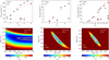 |
Fig. 4 Results from SiO, CS, and SiS analysis for IK Tau. The top panels show the observed intensities (see Table A.4) as black filled circles and the calculated ones of the best-fit model as red empty circles. The bottom panels show χ2 as a function of the logarithm of the e-folding radius, log re, and the logarithm of the fractional abundance relative to H2, log ƒ0. The white contours correspond to 1, 2, and 3σ levels. Similar plots for IRC +10216 are shown in Fig. 5 and for other stars in Fig. A.4 (SiO), Fig. A.5 (CS), and Fig. A.6 (SiS). |
Parameters from the χ2 analysis for SiO, CS, and SiS.
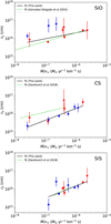 |
Fig. 6 e-folding radii derived in this study as a function of the envelope density proxy, Ṁ/υ∞ for SiO (upper panel), CS (middle panel), and SiS (lower panel). Blue symbols correspond to O-rich envelopes and red ones to C-rich sources. The resulting linear fits are also plotted and compared with fits from previous studies. |
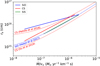 |
Fig. 7 Relation between radial extent and envelope density according to the empirical fits and to the photodissociation model. The solid lines are the empirical fits given by Eqs. (8)–(10), and the dotted lines are the predictions from the photodissociation model using different photodis-sociation rates from the literature (see text). |
5 Conclusions
We carried out an observational study of SiO, CS, and SiS in AGB envelopes, with the aim being to constrain their radial extent in envelopes of different density and chemical type. We find that for the three molecules, the envelope size increases with increasing envelope density, in agreement with previous observational studies. We also find that at high envelope densities, Ṁ/υ∞ > 10–6 M⊙ yr–1 km–1 s, the three molecules show a similar radial extent, while for decreasing envelope densities SiO, CS, and SiS become more differentiated with respect to their radial extent, which is in line with expectations based on a simple photodissociation model. At low envelope densities, we find that molecules extend farther in the following order: SiS → CS → SiO. The scarcity of both interferometric studies and data on the photodissociation of the three molecules prevents us from obtaining solid confirmation or refutation of this scheme. We argue that further modeling studies combining single-dish and interferometric data and an investigation of the photodissociation of SiO, CS, and SiS should allow us to obtain a clearer picture of the radial extent of these molecules in AGB envelopes.
Data availability
The figures and tables of the appendix of this article are available on the public repository zenodo.
Acknowledgements
We acknowledge funding support from Spanish Ministerio de Ciencia e Innovación through grants AYA2016-75066-C2-1-P, PID2019-106110GB-I00, PID2019-107115GB-C21, PID2019-105203GB-C21, PID2019-105203GB-C22, PID2020-117034RJ-I00, and PIE 202250I097, and from the European Research Council (ERC Grant 610256: NANOCOSMOS). Calculations in this work were run at the SGAI-CSIC supercomputer DRAGO and the Galicia Supercomputing Center (CESGA). This work has made use of data from the European Space Agency (ESA) mission Gaia (https://www.cosmos.esa.int/gaia), processed by the Gaia Data Processing and Analysis Consortium (DPAC, https://www.cosmos.esa.int/web/gaia/dpac/consortium). Funding for the DPAC has been provided by national institutions, in particular the institutions participating in the Gaia Multilateral Agreement. This work made also use of the VizieR catalogue access tool, CDS, Strasbourg, France (DOI: 10.26093/cds/vizier). The original description of the VizieR service was published in Ochsenbein et al. (2000). This publication makes use of data products from the Wide-field Infrared Survey Explorer, which is a joint project of the University of California, Los Angeles, and the Jet Propulsion Laboratory/California Institute of Technology, and NEOWISE, which is a project of the Jet Propulsion Laboratory/California Institute of Technology. WISE and NEOWISE are funded by the National Aeronautics and Space Administration. The Pan-STARRS1 Surveys (PS1) and the PS1 public science archive have been made possible through contributions by the Institute for Astronomy, the University of Hawaii, the Pan-STARRS Project Office, the Max-Planck Society and its participating institutes, the Max Planck Institute for Astronomy, Heidelberg and the Max Planck Institute for Extraterrestrial Physics, Garching, The Johns Hopkins University, Durham University, the University of Edinburgh, the Queen’s University Belfast, the Harvard-Smithsonian Center for Astrophysics, the Las Cumbres Observatory Global Telescope Network Incorporated, the National Central University of Taiwan, the Space Telescope Science Institute, the National Aeronautics and Space Administration under Grant No. NNX08AR22G issued through the Planetary Science Division of the NASA Science Mission Directorate, the National Science Foundation Grant No. AST-1238877, the University of Maryland, Eotvos Lorand University (ELTE), the Los Alamos National Laboratory, and the Gordon and Betty Moore Foundation. This publication makes use of data products from the Two Micron All Sky Survey, which is a joint project of the University of Massachusetts and the Infrared Processing and Analysis Center/California Institute of Technology, funded by the National Aeronautics and Space Administration and the National Science Foundation. We are grateful to the anonymous referee for his/her a constructive report.
References
- Adam, C., & Ohnaka, K. 2019, A&A, 628, A132 [NASA ADS] [CrossRef] [EDP Sciences] [Google Scholar]
- Agúndez, M., Fonfria, J. P., Cernicharo, J., et al. 2012, A&A, 543, A48 [NASA ADS] [CrossRef] [EDP Sciences] [Google Scholar]
- Agúndez, M., Cernicharo, J., Quintana-Lacaci, G., et al. 2017, A&A, 601, A4 [Google Scholar]
- Agúndez, M., Roueff, E., Le Petit, F., & Le Bourlot, J. 2018, A&A, 616, A19 [Google Scholar]
- Agúndez, M., Martínez, J. I., de Andres, P. L., et al. 2020, A&A, 637, A59 [CrossRef] [EDP Sciences] [PubMed] [Google Scholar]
- Andriantsaralaza, M., Ramstedt, S., Vlemmings, W. H. T., & De Beck, E. 2022, A&A, 667, A74 [NASA ADS] [CrossRef] [EDP Sciences] [Google Scholar]
- Balança, C., & Dayou, F. 2017, MNRAS, 469, 1673 [CrossRef] [Google Scholar]
- Balança, C., Dayou, F., Faure, A., et al. 2018, MNRAS, 479, 2692 [CrossRef] [Google Scholar]
- Beichman, C. A., Neugebauer, G., Habing, H. J., Clegg, P. E., & Chester, T. J. 1988, Infrared Astronomical Satellite (IRAS) Catalogs and Atlases, 1, Explanatory Supplement [Google Scholar]
- Bergeat, J., Knapik, A., & Rutily, B. 2001, A&A, 369, 178 [NASA ADS] [CrossRef] [EDP Sciences] [Google Scholar]
- Bieging, J. H., Shaked, S., & Gensheimer, P. D. 2000, ApJ, 543, 897 [NASA ADS] [CrossRef] [Google Scholar]
- Bohlin, R. C., Savage, B. D., & Drake, J. F. 1978, ApJS, 224, 132 [NASA ADS] [Google Scholar]
- Bruna, P. J., Kammer, W. E., & Vasudevan, K. 1975, Chem. Phys., 9, 91 [NASA ADS] [CrossRef] [Google Scholar]
- Bujarrabal, V., Fuente, A., & Omont, A. 1994, A&A, 285, 247 [NASA ADS] [Google Scholar]
- Castro-Carrizo, A., Quintana-Lacaci, G., Neri, R., et al. 2010, A&A, 523, A59 [NASA ADS] [CrossRef] [EDP Sciences] [Google Scholar]
- Cecchi-Pestellini, C., Bodo, E., Balakrishnan, N., & Dalgarno, A. 2002, ApJ, 571, 1015 [NASA ADS] [CrossRef] [Google Scholar]
- Cernicharo, J., Guélin, M., & Kahane, C. 2000, A&AS, 142, 181 [NASA ADS] [CrossRef] [EDP Sciences] [Google Scholar]
- Cernicharo, J., Marcelino, N., Agúndez, M., & Guélin, M. 2015, A&A, 575, A91 [NASA ADS] [CrossRef] [EDP Sciences] [Google Scholar]
- Chambers, K. C., Magnier, E. A., Metcalfe, N., et al. 2019, [arXiv:1612.05560] [Google Scholar]
- Chandra, S., Kegel, W. H., Le Roy, R. J., & Hertenstein, T. 1995, A&AS, 114, 175 [NASA ADS] [Google Scholar]
- Daniel, F., Agúndez, M., Cernicharo, J., et al. 2012, A&A, 542, A37 [NASA ADS] [CrossRef] [EDP Sciences] [Google Scholar]
- Danilovich, T., Teyssier, D., Justtanont, K., et al. 2015, A&A, 581, A60 [NASA ADS] [CrossRef] [EDP Sciences] [Google Scholar]
- Danilovich, T., Ramstedt, S., Gobrecht, D., et al. 2018, A&A, 617, A132 [NASA ADS] [CrossRef] [EDP Sciences] [Google Scholar]
- Danilovich, T., Richards, A. M. S., Karakas, A. I., et al. 2019, MNRAS, 484, 494 [CrossRef] [Google Scholar]
- Dayou, F., & Balança, C. 2006, A&A, 459, 297 [NASA ADS] [CrossRef] [EDP Sciences] [Google Scholar]
- De Beck, E., Decin, L., de Koter, A., et al. 2010, A&A, 523, A18 [NASA ADS] [CrossRef] [EDP Sciences] [Google Scholar]
- Decin, L., Justtanont, K., De Beck, E., et al. 2010, A&A, 521, A4 [Google Scholar]
- Denis-Alpizar, O., Stoecklin, T., Guilloteau, S., & Dutrey, A. 2018, MNRAS, 478, 1811 [Google Scholar]
- Drira, I., Huré, J. M., Spielfiedel, A., et al. 1997, A&A, 319, 720 [NASA ADS] [Google Scholar]
- Egan, M. P., Price, S. D., Kraemer, K. E., et al. 2003, Air Force Research Laboratory Technical Report, AFRL-VS-TR-2003-1589 [Google Scholar]
- Flewelling, H. A., Magnier, E. A., Chambers, K. C., et al. 2020, The Astrophys-ical Journal Supplement Series, 251, 62 [Google Scholar]
- Fonfría Expósito, J. P., Agúndez, M., Tercero, B., et al. 2006, ApJ, 646, L127 [CrossRef] [Google Scholar]
- Fonfría, J. P., DeWitt, C. N., Montiel, E. J., et al. 2022, ApJ, 927, L33 [CrossRef] [Google Scholar]
- Gaia Collaboration (Vallenari, A., et al.) 2023, A&A, 674, A1 [NASA ADS] [CrossRef] [EDP Sciences] [Google Scholar]
- Gendriesch, R., Lewen, F., Klapper, G., et al. 2009, A&A, 497, 927 [NASA ADS] [CrossRef] [EDP Sciences] [Google Scholar]
- González Delgado, D., Olofsson, H., Kerschbaum, F., et al. 2003, A&A, 411, 123 [Google Scholar]
- Goorvitch, D. 1994, ApJS, 95, 535 [NASA ADS] [CrossRef] [Google Scholar]
- Groenewegen, M. A. T., & Whitelock, P. A. 1996, MNRAS, 281, 1347 [NASA ADS] [CrossRef] [Google Scholar]
- Groenewegen, M. A. T. 2017, A&A, 606, A67 [NASA ADS] [CrossRef] [EDP Sciences] [Google Scholar]
- Groenewegen, M. A. T., & Saberi, M. 2021, A&A, 649, A172 [NASA ADS] [CrossRef] [EDP Sciences] [Google Scholar]
- Groenewegen, M. A. T., Whitelock, P. A., Smith, C. H., & Kerschbaum, F. 1998, MNRAS, 293, 18 [NASA ADS] [CrossRef] [Google Scholar]
- Groenewegen, M. A. T., Sevenster, M., Spoon, H. W. W., & Pérez, I. 2002, A&A, 390, 511 [NASA ADS] [CrossRef] [EDP Sciences] [Google Scholar]
- Groenewegen, M. A. T., Barlow, M. J., Blommaert, J. A. D. L., et al. 2012, A&A, 543, A8 [NASA ADS] [CrossRef] [EDP Sciences] [Google Scholar]
- Guélin, M., Patel, N. A., Bremer, M., et al. 2018, A&A, 610, A4 [NASA ADS] [CrossRef] [EDP Sciences] [Google Scholar]
- Heays, A. N., Bosman, A. D., & van Dishoeck, E. F. 2017, A&A, 602, A105 [NASA ADS] [CrossRef] [EDP Sciences] [Google Scholar]
- Höfner, S., & Olofsson, H. 2018, A&A Rev., 26, 1 [CrossRef] [Google Scholar]
- Hogerheijde, M. R., & van der Tak, F. F. S. 2000, A&A, 362, 697 [NASA ADS] [Google Scholar]
- Ishihara, D., Onaka, T., Kataza, H., et al. 2010, A&A, 514, A1 [NASA ADS] [CrossRef] [EDP Sciences] [Google Scholar]
- Ivezić, ?. & Elitzur, M. 1997, MNRAS, 287, 799 [CrossRef] [Google Scholar]
- Justtanont, K., Khouri, T., Maercker, M., et al. 2012, A&A, 537, A144 [NASA ADS] [CrossRef] [EDP Sciences] [Google Scholar]
- Karovicova, I., Wittkowski, M., Ohnaka, K., et al. 2013, A&A, 560, A75 [NASA ADS] [CrossRef] [EDP Sciences] [Google Scholar]
- Kłos, J., & Lique, F. 2008, MNRAS, 390, 239 [CrossRef] [Google Scholar]
- Lang, D., 2014, AJ, 147, 108 [Google Scholar]
- Lique, F., & Spielfiedel, A. 2007, A&A, 462, 1179 [NASA ADS] [CrossRef] [EDP Sciences] [Google Scholar]
- Lique, F., Spielfiedel, A., & Cernicharo, J. 2006, A&A, 451, 1125 [NASA ADS] [CrossRef] [EDP Sciences] [Google Scholar]
- Lucas, R., Bujarrabal, V., Guilloteau, S., et al. 1992, A&A, 262, 491 [NASA ADS] [Google Scholar]
- Mainzer, A., Bauer, J., Grav, T., et al. 2011, ApJ, 731, 53 [Google Scholar]
- Massalkhi, S., Agúndez, M., Cernicharo, J., et al. 2018, A&A, 611, A29 [CrossRef] [EDP Sciences] [PubMed] [Google Scholar]
- Massalkhi, S., Agúndez, M., & Cernicharo, J. 2019, A&A, 628, A62 [CrossRef] [EDP Sciences] [PubMed] [Google Scholar]
- Massalkhi, S., Agúndez, M., Cernicharo, J., & Velilla-Prieto, L. 2020, A&A, 641, A57 [NASA ADS] [CrossRef] [EDP Sciences] [Google Scholar]
- Meisner, A. M., Lang, D., & Schlegel, D. J. 2017a, AJ, 153, 38 [Google Scholar]
- Meisner, A. M., Lang, D., & Schlegel, D. J. 2017b, AJ, 154, 161 [NASA ADS] [CrossRef] [Google Scholar]
- Morris, M., & Jura, M. 1983, ApJ, 264, 546 [Google Scholar]
- Müller, H. S. P., Schlöder, F., Stutzki, J., & Winnewiser, G. 2005, J. Mol. Struct., 742, 215 [CrossRef] [Google Scholar]
- Müller, H. S. P., McCarthy, M. C., Bizzocchi, L., et al. 2007, PCCP, 9, 1579 [CrossRef] [Google Scholar]
- Neri, R., Kahane, C., Lucas, R., et al. 1998, A&AS, 130, 1 [NASA ADS] [CrossRef] [EDP Sciences] [Google Scholar]
- Ochsenbein, F., Bauer, P., & Marcout, J. 2000, A&AS, 143, 23 [NASA ADS] [CrossRef] [EDP Sciences] [Google Scholar]
- Olivier, E. A., Whitelock, P., & Marang, F. 2001, MNRAS, 326, 490 [NASA ADS] [CrossRef] [Google Scholar]
- Olofsson, H., Lindqvist, M., Nyman, L.-Å., & Winnberg, A. 1998, A&A, 329, 1059 [NASA ADS] [Google Scholar]
- Olofsson, H., González Delgado, D., Kerschbaum, F., & Schöier, F. L. 2002, A&A, 391, 1053 [NASA ADS] [CrossRef] [EDP Sciences] [Google Scholar]
- Pardo, J. R., Cernicharo, J., Tercero, B., et al. 2022, A&A, 658, A39 [NASA ADS] [CrossRef] [EDP Sciences] [Google Scholar]
- Pattillo, R. J., Cieszewski, R., Stancil, P. C., et al. 2018, ApJ, 858, 10 [NASA ADS] [CrossRef] [Google Scholar]
- Perrin, G., Coudé du Foresto, V., Ridgway, S. T., et al. 1999, A&A, 345, 221 [NASA ADS] [Google Scholar]
- Pety, J. 2005, in SF2A-2005: Semaine de l’Astrophysique Francaise, eds. F. Casoli et al. (Les Ulis: EDP-Sciences), 721 [Google Scholar]
- Piñeiro, A. L., Tipping, R. H., & Chackerian, C. 1987, J. Mol. Spectr., 125, 91 [CrossRef] [Google Scholar]
- Price, S. D., Egan, M. P., Carey, S. J., et al. 2001, AJ, 121, 2819 [Google Scholar]
- Price, S. D. Smith, B. J., Kuchar, T. A., et al. 2010, ApJS, 190, 203 [NASA ADS] [CrossRef] [Google Scholar]
- Ramstedt, S., & Olofsson, H. 2014, A&A, 566, A145 [NASA ADS] [CrossRef] [EDP Sciences] [Google Scholar]
- Ramstedt, S., Schöier, F. L., Olofsson, H., & Lundgren, A. A. 2008, A&A, 487, 645 [NASA ADS] [CrossRef] [EDP Sciences] [Google Scholar]
- Ramstedt, S., Vlemmings, W. H. T., Doan, L., et al. 2020, A&A, 640, A133 [EDP Sciences] [Google Scholar]
- Raymonda, J. W., Muenter, J. S., & Klemperer, W. A. 1970, J. Chem. Phys., 52, 3458 [NASA ADS] [CrossRef] [Google Scholar]
- Ridgway, S. T., & Keady, J. J. 1988, ApJ, 326, 843 [NASA ADS] [CrossRef] [Google Scholar]
- Rothman, L. S., Jacquemart, D., Barbe, A., et al. 2005, JQSRT, 96, 139 [NASA ADS] [CrossRef] [Google Scholar]
- Saberi, M., Vlemmings, W. H. T., De Beck, E. 2019, A&A, 625, A81 [NASA ADS] [CrossRef] [EDP Sciences] [Google Scholar]
- Sahai, R., & Bieging, J. H. 1993, AJ, 105, 595 [NASA ADS] [CrossRef] [Google Scholar]
- Sanz, M. E., McCarthy, M. C., & Thaddeus, P. 2003, J. Chem. Phys., 119, 11715 [NASA ADS] [CrossRef] [Google Scholar]
- Schöier, F. L., & Olofsson, H. 2001, A&A, 368, 969 [Google Scholar]
- Schöier, F. L., Ryde, N., & Olofsson, H. 2002, A&A, 391, 577 [NASA ADS] [CrossRef] [EDP Sciences] [Google Scholar]
- Schöier, F. L., Olofsson, H., Wong, T., et al. 2004, A&A, 422, 651 [NASA ADS] [CrossRef] [EDP Sciences] [Google Scholar]
- Schöier, F. L., Olofsson, H., & Lundgren, A. A. 2006a, A&A, 454, 247 [NASA ADS] [CrossRef] [EDP Sciences] [Google Scholar]
- Schöier, F. L., Fong, D., Olofsson, H., et al. 2006b, ApJ, 649, 965 [CrossRef] [Google Scholar]
- Schöier, F. L., Bast, J., Olofsson, H., & Lindqvist, M. 2007, A&A, 473, 871 [NASA ADS] [CrossRef] [EDP Sciences] [Google Scholar]
- Schöier, F. L., Ramstedt, S., Olofsson, H., et al. 2013, A&A, 550, A78 [Google Scholar]
- Scicluna, P., Kemper, F., McDonald, I., et al. 2022, MNRAS, 512, 1091 [NASA ADS] [CrossRef] [Google Scholar]
- Skrutskie, M. F., Cutri, R. M., Stiening, R., et al. 2006, AJ, 131, 1163 [NASA ADS] [CrossRef] [Google Scholar]
- Smith, B. J., Price, S. D., & Baker, R. I. 2004, ApJS, 154, 673 [NASA ADS] [CrossRef] [Google Scholar]
- Stark, G., Yoshino, K., & Smith, P. L. 1987, J. Mol. Spectr., 124, 420 [NASA ADS] [CrossRef] [Google Scholar]
- Suh, K.-W. 1999, MNRAS, 304, 389 [NASA ADS] [CrossRef] [Google Scholar]
- Suh, K.-W. 2000, MNRAS, 315, 740 [NASA ADS] [CrossRef] [Google Scholar]
- Tercero, F., López-Pérez, J. A., Gallego, J. D., et al. 2021, A&A, 645, A37 [EDP Sciences] [Google Scholar]
- Toboła, R., Lique, F., Klos, J., & Chalasinski, G. 2008, J. Phys. B At. Mol. Phys., 41, 155702 [CrossRef] [Google Scholar]
- Tsuji, T. 1973, A&A, 23, 411 [NASA ADS] [Google Scholar]
- van Dishoeck, E. F. 1988, Astrophys. Space Sci. Lib., 146, 49 [NASA ADS] [CrossRef] [Google Scholar]
- van Dishoeck, E. F., Jonkheid, B., & van Hemert, M. C. 2006, Faraday Discuss., 133, 231 [Google Scholar]
- van Loon, J. Th., Cioni, M.-R. L., Zijlstra, A. A., & Loup, C. 2005, A&A, 438, 273 [NASA ADS] [CrossRef] [EDP Sciences] [Google Scholar]
- Velilla-Prieto, L., Sánchez-Contreras, C., Cernicharo, J., et al. 2017, A&A, 597, A25 [NASA ADS] [CrossRef] [EDP Sciences] [Google Scholar]
- Velilla-Prieto, L., Cernicharo, J., Agúndez, M., et al. 2019, A&A, 629, A146 [NASA ADS] [CrossRef] [EDP Sciences] [Google Scholar]
- Verbena, J. L., Bujarrabal, V., Alcolea, J., et al. 2019, A&A, 624, A107 [EDP Sciences] [Google Scholar]
- Whitelock, P., Menzies, J., Feast, M., et al. 1994, MNRAS, 267, 711 [NASA ADS] [CrossRef] [Google Scholar]
- Whitelock, P. A., Feast, M. W., & van Leeuwen, F. 2008, MNRAS, 386, 313 [CrossRef] [Google Scholar]
- Winnewiser, G., & Cook, R. L. 1968, J. Mol. Spectr., 28, 266 [NASA ADS] [CrossRef] [Google Scholar]
- Winnewiser, G., Belov, S. P., Klaus, Th., & Schieder, R. 1997, J. Mol. Spectr., 184, 468 [NASA ADS] [CrossRef] [Google Scholar]
- Wirsich, J. 1994, ApJ, 424, 370 [NASA ADS] [CrossRef] [Google Scholar]
- Woods, P. M., Schöier, F. L., Nyman, L.-Å., & Olofsson, H. 2003, A&A, 402, 617 [NASA ADS] [CrossRef] [EDP Sciences] [Google Scholar]
- Wright, E. L., Eisenhardt, P. R. M., Mainzer, A., et al. 2010, AJ, 140, 1868 [NASA ADS] [CrossRef] [Google Scholar]
- Xu, Z., Luo, N., Federman, S. R., et al. 2019, ApJ, 882, 86 [NASA ADS] [CrossRef] [Google Scholar]
- Yang, B., Stancil, P. C., Balakrishnan, N., & Forrey, R. C. 2010, ApJ, 718, 1062 [Google Scholar]
All Tables
All Figures
|
Fig. 1 Results from SED analysis for IK Tau and IRC +10216. The left panels show the observed fluxes in blue (see Table A.2) and the calculated SED from the best DUSTY model in red. The right panels show χ2 as a function of the dust temperature at the condensation radius, Td(rc), and the logarithm of the dust optical depth at 10 µm, log τ10. The white contours correspond to 1, 2, and 3σ levels. Similar plots for other stars are shown in Fig. A.2. |
| In the text | |
|
Fig. 2 Results from CO analysis for IK Tau. The left panel shows the observed intensities (see Table A.3) as black filled circles and the calculated ones as red empty circles. The right panel shows χ2 as a function of the logarithm of the mass-loss rate, log Ṁ, and the exponent of the gas kinetic temperature radial profile, δ. The white contours correspond to 1, 2, and 3σ levels. Similar plots for other stars are shown in Fig. A.3. |
| In the text | |
|
Fig. 3 Best-fit CO model for IRC +10216. The observed intensities (see Table A.3) are represented by black filled circles and the calculated ones by red empty circles. |
| In the text | |
|
Fig. 4 Results from SiO, CS, and SiS analysis for IK Tau. The top panels show the observed intensities (see Table A.4) as black filled circles and the calculated ones of the best-fit model as red empty circles. The bottom panels show χ2 as a function of the logarithm of the e-folding radius, log re, and the logarithm of the fractional abundance relative to H2, log ƒ0. The white contours correspond to 1, 2, and 3σ levels. Similar plots for IRC +10216 are shown in Fig. 5 and for other stars in Fig. A.4 (SiO), Fig. A.5 (CS), and Fig. A.6 (SiS). |
| In the text | |
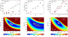 |
Fig. 5 Same as Fig. 4 but for IRC +10216. |
| In the text | |
|
Fig. 6 e-folding radii derived in this study as a function of the envelope density proxy, Ṁ/υ∞ for SiO (upper panel), CS (middle panel), and SiS (lower panel). Blue symbols correspond to O-rich envelopes and red ones to C-rich sources. The resulting linear fits are also plotted and compared with fits from previous studies. |
| In the text | |
|
Fig. 7 Relation between radial extent and envelope density according to the empirical fits and to the photodissociation model. The solid lines are the empirical fits given by Eqs. (8)–(10), and the dotted lines are the predictions from the photodissociation model using different photodis-sociation rates from the literature (see text). |
| In the text | |
Current usage metrics show cumulative count of Article Views (full-text article views including HTML views, PDF and ePub downloads, according to the available data) and Abstracts Views on Vision4Press platform.
Data correspond to usage on the plateform after 2015. The current usage metrics is available 48-96 hours after online publication and is updated daily on week days.
Initial download of the metrics may take a while.