| Issue |
A&A
Volume 688, August 2024
|
|
|---|---|---|
| Article Number | A66 | |
| Number of page(s) | 8 | |
| Section | Planets and planetary systems | |
| DOI | https://doi.org/10.1051/0004-6361/202450095 | |
| Published online | 02 August 2024 | |
Follow-up LOFAR observations of the τ Boötis exoplanetary system
1
Department of Astronomy and Carl Sagan Institute, Cornell University,
Ithaca,
NY,
USA
e-mail: This email address is being protected from spambots. You need JavaScript enabled to view it.
2
Laboratoire de Physique et Chimie de l’Environnement et de l’Espace (LPC2E) Université d’Orléans/CNRS,
Orléans,
France
3
Observatoire Radioastronomique de Nançay (ORN), Observatoire de Paris, PSL Research University, CNRS, Univ. Orléans, OSUC,
18330
Nançay,
France
4
LESIA, Observatoire de Paris, CNRS, PSL,
Meudon,
France
Received:
22
March
2024
Accepted:
2
May
2024
Abstract
Context. Observing the radio emission from exoplanets is among the most promising methods to detect their magnetic fields and a measurement of an exoplanetary magnetic field will help constrain the planet’s interior structure, star-planet interactions, atmospheric escape and dynamics, and habitability. Recently, circularly polarized bursty and slow emission from the τ Boötis (τ Boo) exoplanetary system was tentatively detected using LOFAR (LOW-Frequency ARray) beamformed observations. If confirmed, this detection will be a major contribution to exoplanet science. However, follow-up observations are required to confirm this detection.
Aims. Here, we present such follow-up observations of the τ Boo system using LOFAR. These observations cover 70% of the orbital period of τ Boo b including the orbital phases of the previous tentative detections.
Methods. We used the BOREALIS pipeline to mitigate radio frequency interference and to search for bursty and slowly varying radio signals. BOREALIS was previously used to find the tentative radio signals from τ Boo.
Results. Our new observations do not show any signs of bursty or slow emission from the τ Boötis exoplanetary system.
Conclusions. The cause for our non-detection is currently degenerate. It is possible that the tentative radio signals were an unknown instrumental systematic or that we are observing variability in the planetary radio emission due to changes in its host star. More radio data (preferably multi-site) and ancillary observations (e.g. magnetic maps) are required to further investigate the potential radio emission from the τ Boötis exoplanetary system.
Key words: planets and satellites: aurorae / planets and satellites: gaseous planets / planets and satellites: magnetic fields / planet-star interactions
NHFP Sagan Fellow.
© The Authors 2024
 Open Access article, published by EDP Sciences, under the terms of the Creative Commons Attribution License (https://creativecommons.org/licenses/by/4.0), which permits unrestricted use, distribution, and reproduction in any medium, provided the original work is properly cited.
This article is published in open access under the Subscribe to Open model. This email address is being protected from spambots. You need JavaScript enabled to view it. to support open access publication.
1 Introduction
A confirmed direct detection of exoplanetaгy radio emission has been elusive for decades. Observing the radio emission from exoplanets is among the most promising methods to detect their magnetic fields (Grießmeier 2015) and a measurement of an exoplanetary magnetic field will help constrain the planet’s interior structure, star-planet interactions, and atmospheric escape (e.g. Zarka et al. 2015; Grießmeier 2015, 2017; Griessmeier 2018; Lazio et al. 2016, 2019; Lazio 2018; Zarka 2018). A magnetic field measurement can help also help break degeneracies in the mass-radius diagram (Lazio et al. 2019). Additionally, atmospheric dynamics may be influenced by the presence of a planetary magnetic field (e.g. Perna et al. 2010a; Rauscher & Menou 2013; Rogers & Komacek 2014; Hindle et al. 2021) and Ohmic dissipation might be one of the factors causing the anomalously large radii of hot Jupiters (e.g. Perna et al. 2010a,b; Knierim et al. 2022). Finally, a magnetic field might be one of the many properties needed on Earth-like exoplanets to sustain their habitability (e.g. Grießmeier et al. 2005b, 2015, 2016; Lammer et al. 2009; Kasting 2010; Owen & Adams 2014; Lazio et al. 2010a, 2016; Meadows & Barnes 2018; McIntyre et al. 2019; Gronoff et al. 2020; Green et al. 2021b).
Observations of auroral radio emissions produced via the Cyclotron Maser Instability (CMI) mechanism (Wu & Lee 1979; Zarka 1998; Treumann 2006) have been used to directly measure the magnetic field strengths of some of the magnetized planets in our Solar System (Burke & Franklin 1955; Zarka 1998). CMI radio signals are emitted at the local electron cyclotron frequency in the source region. Hence, the maximum gyrofrequency is directly proportional to the maximum magnetic field near the planetary surface. CMI radio emission is circularly polarized, beamed, and time-variable (e.g. Zarka 1998; Zarka et al. 2004).
Many theoretical and observational studies have focused on studying exoplanetary radio emissions over the past few decades. The reviews by Zarka et al. (2015) and Grießmeier (2015, 2017) cover the subject in great detail. A large body of theoretical work1 has been published since the foundational theoretical studies of Zarka et al. (1997, 2001), Farrell et al. (1999), and Zarka (2007). Some of these studies aim to develop theoretical models that can predict the frequency and intensity of radio emissions observed from Earth. A variety of scaling laws have been developed to estimate the magnetic field strengths of exoplanets (e.g. Farrell et al. 1999; Sánchez-Lavega 2004; Grießmeier et al. 2007b; Christensen et al. 2009; Christensen 2010; Reiners & Christensen 2010). Likewise, the Radio-Magnetic Bode’s law is a common approach for estimating the radio emission intensity of these planets (e.g. Farrell et al. 1999; Lazio et al. 2004; Zarka 2007, 2018; Grießmeier et al. 2007b; Grießmeier 2017; Zarka et al. 2018).
Over the past few decades, there have been many exoplanet radio observing campaigns, but none of these observations have resulted in an unambiguous detection2. There have been a few tentative detections (Lecavelier des Etangs et al. 2013; Sirothia et al. 2014; Vasylieva 2015; Bastian et al. 2018), but none of them have been confirmed by follow-up observations. The many degenerate reasons for the non-detections are discussed in great detail in the review articles Zarka et al. (2015) and Grießmeier (2015, 2017). Some reasons for the non-detections could be that the observations were not sensitive enough (e.g. Bastian et al. 2000), there was no emission at the observed frequencies due to a low magnetic field strength (e.g. Hallinan et al. 2013), Earth was outside the CMI beaming pattern (Hess & Zarka 2011; Ashtari et al. 2022), and/or the CMI mechanism was not operating (e.g. plasma frequency of the planet’s ionosphere was greater than the cyclotron frequency; Grießmeier et al. 2007b; Weber et al. 2017a,b, 2018; Lamy et al. 2018). By contrast, advancement has been made in detecting free-floating planets near the brown dwarf boundary (Kao et al. 2016, 2018) and stellar emission potentially created by star-planet interactions (e.g. Vedantham et al. 2020; Callingham et al. 2021; Pérez-Torres et al. 2021; Pineda & Villadsen 2023; Trigilio et al. 2023; Blanco-Pozo et al. 2023).
In a recent study, circularly polarized bursty and slow emission from the τ Boötis (τ Boo) exoplanetary system was tentatively detected by Turner et al. (2021, hereafter T21) using LOFAR (LOw Frequency ARray; van Haarlem et al. 2013) beamformed observations taken in 2017. The slow and burst emission were seen at orbital phases of 0.65 and 0.8, respectively, in relation to the τ Boo b’s periastron (see Fig. 1). The bursty emission was seen from 15–21 MHz, while the slower emission was present in the 21–30 MHz range. T21 did not identify any plausible sources of false positives for the bursty emission, but when it came to the slower emission, uncertainty arose due to the possibility of unknown systematic effects causing the signal. Assuming an astronomical origin for the signal, T21 concluded that the signals originated from the τ Boo system, with the most likely cause being CMI radio emission from the exoplanet τ Boo b. Under the premise of a planetary origin for the radio signals, T21 derived planetary magnetic field constraints that are consistent with theoretical predictions (Grießmeier et al. 2007b; Grießmeier 2017). More recent calculations (Mauduit et al. 2023; Ashtari et al. 2022) using an updated version of these predictions also yielded magnetic moment and flux density values that aligned with the earlier theoretical estimates, in addition to matching the observed phases and the handedness of the circular polarization (Ashtari et al. 2022). Follow-up observations were highly advocated by T21 to confirm their tentative detections and to search for periodicity in the signal.
Motivated by the tentative detection of radio emission from τ Boo, we performed a large follow-up campaign in 2020. This campaign was coordinated between four different radio telescopes including LOFAR and NenuFAR (New Extension in Nançay Upgrading LOFAR; Zarka et al. 2020). In this paper, we only present the LOFAR data of τ Boo since the sensitivity of LOFAR has been well characterized using simulated Jupiter radio emission data (Turner et al. 2019, hereafter T19) and a complete data reduction pipeline is available (T19; T21). A preliminary analysis of the NenuFAR data is presented elsewhere (Turner et al. 2023).
In this paper, Sects. 2, 3, and 4 describe the τ Boo observations, data processing, and data analysis, respectively. Section 5 discusses the possible reasons for our non-detections and future steps.
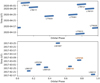 |
Fig. 1 Orbital phase coverage for the LOFAR observations of τ Boo b. The observations from this study and Turner et al. (2021) are shown in the top and bottom panels, respectively. The orbital phase was calculated relative to periastron of τ Boo b using the ephemeris (period = 3.312463 days, T(0)per = 2446 957.81 JD) from Wang & Ford (2011). The τ Boo LOFAR observations with the tentative detections (L569119 and L570725) from Turner et al. (2021) are displayed in red. |
2 Observations
All of the observations presented here were taken with the Low Band Antenna (LBA) of LOFAR (van Haarlem et al. 2013) using beamformed mode (Stappers et al. 2011). We obtained 8 exoplanet observations (each 8 h long) for a total of 64 h, plus 8 observations of the pulsar B0809+74 totaling 82 min. Similar to our previous studies (Turner et al. 2017a, 2023; T19; T21), the pulsar observations are used as a calibrator to study systematics in the data and to ensure the reliability of the processing. An example OFF-beam dynamic spectrum is shown in Fig. 2. The dates and times of the observations can be found in Table 1. The setup of the observations can be found in Table 2; it is similar to that in T21. Most importantly, we ensure we cover the 15–30 MHz range where T21 detected their tentative signals. We only present the Stokes-V3 in this paper since the tentative detections were seen in Stokes-V (T21).
In this study, we compare our on-target beam (“ON-beam”) to several simultaneous beams pointing to nearby locations in the sky (“OFF-beam 1”, “OFF-beam 2” and “OFF-beam 3”). This is similar to our previous studies (Turner et al. 2017a; T19; T21) except we now use three OFF-beams instead of two to further investigate systematic effects in the analysis. This method relies on the assumption that the OFF beams can effectively characterize and account for ionospheric fluctuations, radio frequency interference, and any other systematic errors that may be present. The beamformed LOFAR observations of 55 Cancri, υ Andromedae, and τ Boo demonstrated that this assumption holds true (T21).
Our new LOFAR observations cover 70% of the orbit of τ Boo b as seen in Fig. 1. Due to the emission geometry (Hess & Zarka 2011; Ashtari et al. 2022), it is anticipated that the emission will only be directed towards Earth for a limited period. Therefore, the observation windows were selected to ensure the widest possible orbital coverage to maximize the chances to detect beamed emission. Most importantly, we also obtained two new observations around phase 0.65 (2020-04-11 and 2020-05-01) and one new observation around phase 0.8 (2020-04-15) that cover the same phases as the tentative slow emission and burst emission signal from T21, respectively. These phases are most likely to have detectable emission as shown in the modeling of the time-dependent CMI beaming effect by Ashtari et al. (2022).
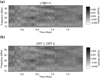 |
Fig. 2 Example dynamic spectrum of the OFF-beam (panel a) and the difference (panel b) between two OFF-beams in Stokes-V for the L780111 (2020-04-29) τ Boo observation. This dynamic spectrum has been processed with BOREALIS. |
Summary of the observations of τ Boötis in LOFAR Cycle 13.
Setup of the LOFAR-LBA beamformed observations of τ Boötis.
3 Data pipeline
All observations were processed with the BOREALIS (Beam-fOrmed Radio Emission AnaLysIS) pipeline (Vasylieva 2015; Turner et al. 2017a; T19; T21). BOREALIS is split into two main components: processing and post-processing. The processing part of BOREALIS performs RFI mitigation, corrects for any large-scale time-frequency (t–f) response variations of the telescope (i.e. gain variations), and rebins the RFI mitigated and corrected data. All parts of the analysis were done exactly as in T21. The RFI mitigation combines four different techniques (Offringa et al. 2010, 2012; Offringa 2012; Zakharenko et al. 2013; Vasylieva 2015) for optimal efficiency and processing time. The t–f response of the telescope is empirically determined assuming a quadratic dependence in time for each frequency. BOREALIS has been extensively tested on pulsar (Turner et al. 2017a) and scaled Jupiter radio emission data (T19) to ensure optimal RFI mitigation and t–f response variation corrections without sacrificing detection capabilities. See Fig. 2 for example OFF-beam dynamic spectrum processed through BOREALIS.
We performed the post-processing of the LOFAR data exactly as in T21. A very detailed description of the burst and slow emission post-processing observables can be found in T19 and T21. A brief summary is given below. The post-processing is performed on the absolute value of the corrected Stokes-V data (as defined in T19). For the slowly varying emission, we calculate the Q1a time series (e.g. Figs. 3a and b) and Q1b integrated spectrum (e.g. Figs. 3c–d) for each beam (ON, OFF1, OFF2, and OFF3). For burst emission, we only use the Q2 and Q4a-f observable quantities. These quantities are designed to find bursty emission (with time scales <~1 min). The Q2 observable is a time series that is created by high-pass filtering the processed dynamic spectrum and integrating over a large frequency range (e.g. 10 MHz) and time resolution (1 s). This integration over a large frequency range is needed to search for faint emission (see e.g. T21). Q2 is calculated separately for each beam (ON, OFF1, OFF2, and OFF3). Q2 can be represented by a “scatter plot” comparing a pair of beams (e.g. the ON and one of the OFF beams, Figs. 4a and b). Next, we calculate the Q4a to Q4f statistical measures to provide a statistical view of the entire observation as individual bursts in the Q2 scatter plots are hard to identify. When examining Q4a-f, the ON and one of the OFF time series are compared to each other; for this, we introduce the difference curve Q4fDiff = Q4f(ON) – Q4f(OFF). We then plot this curve against a reference curve computed from 10 000 draws of purely Gaussian noise. The postprocessing was performed separately over 3 different frequency ranges (15–26 MHz, 15–39 MHz, and 26–29 MHz).
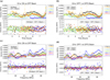 |
Fig. 3 Time series (Q1a: panels a and b) and Integrated spectrum (Q1b: panels c and d) for different beams (ON, OFF-1, OFF-2) for the follow-up LOFAR τ Boötis observations. The two-sigma error bars are shown in the black brackets. Large-scale features can be seen for all dates, however, they change between observations. No distinct emission in the ON-beam is seen when compared to the OFF-beams. There are no large-scale differences seen between the three beams for any date. The third OFF-beam is indistinguishable from the other OFF-beams within the noise. |
4 Data analysis and results
We searched for excess signal in the ON-beam both by eye and using the automated search procedure outlined in T21. To search for a possible detection of burst emission we applied the criteria (N1 to N12) defined in T19 and T21 . We do not find any slow or burst emissions in the observations. The time series (Q1a) and integrated spectra (Q1b) for all beams can be found in Fig. 3. The top and bottom panels of Fig. 3 show the time series and integrated spectra, respectively. Unlike in T21, we do not see a sinusoidal pattern (that may have been caused by imperfect phasing of the array) in the integrated spectrum (Figs. 3c and d). Next, we examine whether there are any systematic differences in the noise between beams. To do this, we tested for the presence of red noise in the difference time series and integrated spectra (bottom panels Figs. 3a–d) for all the observations using the time-averaging method (Pont et al. 2006) and wavelet technique4 (Carter & Winn 2009) as implemented in the EXOMOP code by Turner et al. (2016, 2017b), and found none. Thus any differences in the signals between the ON and OFF beams can be explained purely by Gaussian white noise. The burst statistics were also similar between all ON and OFF beams. An example of the diagnostics for a non-detection can be found in Fig. 4, based on the L776035 (2020-04-15) observation, analyzed within 15–27 MHz. The ON-OFF and OFF-OFF difference curves are very similar to each other. In summary, we did not detect any slow or bursty signals in our data. In Sect. 5, we will discuss the implications of these non-detections and our derived upper-limits.
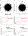 |
Fig. 4 Non-detection of burst emission for τ Boo in the L776035 (2020-04-15) observation between 15 and 27 MHz in Stokes-V (|V′|). Panel a: Q2 for the ON-beam vs. the OFF-beam 2. Panel b: Q2 for the OFF-beam 1 vs. the OFF-beam 2. Panel c: Q4a (number of peaks). Panel d: Q4b (power of peaks). Panel e: Q4e (peak offset). Panel f: Q4f (peak offset). For panels c–f: the black lines are the ON-beam difference with the OFF beam 1 and the red lines are the OFF-beam difference. The dashed lines are statistical limits (1, 2, 3σ) of the difference between all the Q4 values derived using two different Gaussian distributions (each performed 10 000 times). We do not see any excess signal in the ON-beam compared to the OFF-beams. In fact, the OFF-beams show a false-positive weak signal at η ~ 4. |
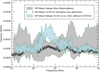 |
Fig. 5 Comparison of the integrated spectra (Q1b) of the LOFAR τ Boötis OFF-beams between the new observations in this paper (gray-shaded area) and those presented (light-blue shaded area) in Turner et al. (2021). We show separately the OFF-beam in the L570725 observation (square black points), where a tentative detection of slow emission was found from Turner et al. (2021). The integrated spectrum for each date in the current observing campaign can be found in Fig. 3. While the OFF-beam in L570725 is abnormal when compared to the rest of the Turner et al. (2021) observations, it is consistent with the new observations. |
5 Discussion
We do not detect any bursty or slow emission in the new LOFAR observations. If the signals in T21 were coming from the planet we could have expected to detect them again at the same phases. However, this assumes no variability in the radio signal and that the signals are from the planet. We discuss these possibilities more below. Our non-detection is consistent with the non-detection of bursty emission from five NenuFAR observations (Turner et al. 2023) taken simultaneously with the LOFAR observation (see Fig. 1 in Turner et al. 2023). Most importantly, both NenuFAR and LOFAR don’t observe bursty emission on April 15, 2020, which covered the same phase as the T21 bursty tentative detection.
5.1 Degenerate causes of the non-detection
There are many different degenerate reasons which could explain our non-detection of emission from τ Boo. We explore the possibilities in greater detail below:
- 1.
The first possibility is that the original slow and/or bursty signals seen by T21 were caused by statistical anomalies or unknown unidentified instrumental systematics. In T21, it was suggested that the OFF beam on the slow emission detection behaved abnormally (the flux on that date was much lower than all the other dates) compared to the rest of the observations. This possibility can be investigated further with the new observations. We find that the OFF beams in the L570725 are not abnormal when compared to the OFF beams in the new 2020 τ Boo observations (see Fig. 5). This suggests that the original slow emission signal may have not been an unknown instrumental systematic but it doesn’t completely it rule out.
- 2.
The planetary emission from τ Boo b might be variable. The expected intensity of the planetary radio emission can differ greatly with stellar rotation (e.g. Grießmeier et al. 2005a, 2007a; Fares et al. 2010; Vidotto et al. 2012; See et al. 2015; Strugarek et al. 2022) and phase of the stellar magnetic cycle (e.g. Fares et al. 2009; Vidotto et al. 2012; See et al. 2015; Elekes & Saur 2023). The latter point is very much a concern since the host star τ Boo is known to undergo a rapid magnetic cycle of 120 days (Mittag et al. 2017; Jeffers et al. 2018). See et al. (2015) showed that the expected radio flux of τ Boo b can disappear entirely for certain stellar rotation phases and also that it can vary (at optimal stellar longitude) by a factor of ~5 along the stellar magnetic cycle. Recently, Elekes & Saur (2023) found using numerical simulations of the τ Boo system that if the magnetic field of the star were to reverse and become anti-aligned with the magnetic field of the planet, the planetary radio emissions would be significantly reduced and could fall below the detection threshold of LOFAR. Unfortunately, no stellar magnetic field measurements exist during the new LOFAR observations. Therefore, we cannot rule out planetary radio emission variability as the cause of our non-detection.
- 3.
It is possible that one of the conditions to allow the CMI mechanism to operate is temporarily violated. For example, an extended and evaporating atmosphere may increase the local electron plasma frequency such that it is greater than the local electron cyclotron frequency, ωp > ωc; (e.g. Weber et al. 2017a,b; Elekes & Saur 2023; Grießmeier et al. 2023). However, for τ Boo b this effect is predicted to not be a problem due to its large mass (Weber et al. 2018). On the other hand, temporal variations could lead to circumstances where the emission does not operate continuously if the planetary magnetic field is as low as estimated by Reiners & Christensen (2010). Evidence suggests that the observed field strengths for brown dwarfs (Kao et al. 2016, 2018) cannot be explained by the Reiners & Christensen (2010) energy flux and magnetic energy density scaling relation. However, it is currently unclear if this contradiction extends to τ Boo b and other hot Jupiters. Therefore, more work is needed to understand whether the plasma conditions at τ Boo b vary such that the conditions for the CMI are not always fulfilled.
- 4.
In contrast to Jupiter’s decametric emissions (Zarka 1998), τ Boo b’s radio emission may not exhibit continuous activity. This would suggest that the magnetospheric dynamics of τ Boo b could be different from those of Jupiter. For instance, the density of the magnetosphere might vary and at times be temporarily depleted in energetic electrons.
To determine the true cause of the potential radio variability of the τ Boo system, it is crucial to conduct an extensive follow-up campaign. To rule out instrumental systematics, multi-site observations are recommended. We also advocate for complimentary imaging observations to follow-up on the τ Boo tentative detection (T21). A detailed comparison of the advantages and drawbacks between beamformed and imaging observations can be found in Sect. 6.3 of T21. It is necessary to monitor the planet’s behavior throughout its orbit and the host star’s magnetic cycle to distinguish between conflicting factors. Additionally, measurements of the star’s magnetic field must be taken during the radio follow-up campaign. Currently, there is an ongoing collaborative campaign utilizing NenuFAR to study τ Boo radio emission and several telescopes (TBL/Neo-Narval and CHFT/ESPaDOnS) to monitor the magnetic field of the host star. The results of this study will be presented in future work.
5.2 Upper-limits on the radio flux density
With our non-detection, we can place an upper limit on the radio emission from the τ Boo system at the time of the observations. We find a 3σ upper limit of 165 mJy from the range 15–39 MHz using the Q1a observable for the slowly varying emission. The noise characteristics of Q1a for the new observations is lower by a factor of 2 than the noise seen in the T21 detection. Using the attenuated Jupiter modeling done in T19, we find for the burst emission an upper limit on the flux density that should less than 105× the peak flux of Jupiter’s decametric burst emission (~5 × 10⁶ Jy; Zarka et al. 2004).
6 Conclusions
In this study, we performed follow-up low-frequency beam-formed radio observations of the τ Boötis (τ Boo) exoplanetary system with LOFAR. Previous LOFAR observations showed tentative hints of a detection possibly originating from the exoplanetary system (Turner et al. 2021). In the new observations, we do not detect any burst or slow emission from τ Boo (Figs. 3–4). The current cause of the non-detection is degenerate (see Sect. 5.1) but could be caused by variability in the planetary radio emission. More radio observations (preferably multi-site) are needed that cover the full orbit of the planet multiple times and at different epochs of the stellar magnetic cycle. Near-simultaneous stellar magnetic maps and stellar monitoring are highly encouraged and needed to disentangle the various competing effects. The newly commissioned NenuFAR and LWA-OVRO are scheduled to observe the τ Boo exoplanetary system and will help investigate the cause of the possible variable emission.
Acknowledgements
J.D. Turner was supported for this work by NASA through the NASA Hubble Fellowship grant #HST-HF2-51495.001-A awarded by the Space Telescope Science Institute, which is operated by the Association of Universities for Research in Astronomy, Incorporated, under NASA contract NAS5-26555. P. Zarka acknowledges funding from the ERC Nº 101020459–Exoradio. This work was supported by the “Programme National de Plané-tologie” (PNP) of CNRS/INSU co-funded by CNES and by the “Programme National de Physique Stellaire” (PNPS) of CNRS/INSU co-funded by CEA and CNES. This research has made use of the Extrasolar Planet Encyclopaedia (exoplanet.eu) maintained by J. Schneider (Schneider et al. 2011), the NASA Exoplanet Archive, which is operated by the California Institute of Technology, under contract with the National Aeronautics and Space Administration under the Exoplanet Exploration Program, and NASA’s Astrophysics Data System Bibliographic Services. This research has also made use of Aladin sky atlas developed at CDS, Strasbourg Observatory, France (Bonnarel et al. 2000; Boch & Fernique 2014). This paper is based on data obtained with the International LOFAR Telescope (ILT) under project codes LC7_013 and LC13_027. LOFAR (van Haarlem et al. 2013) is the Low Frequency Array designed and constructed by ASTRON. It has observing, data processing, and data storage facilities in several countries, that are owned by various parties (each with their own funding sources), and that are collectively operated by the ILT foundation under a joint scientific policy. The ILT resources have benefited from the following recent major funding sources: CNRS-INSU, Observatoire de Paris and Université d'Orléans, France; BMBF, MIWF-NRW, MPG, Germany; Science Foundation Ireland (SFI), Department of Business, Enterprise and Innovation (DBEI), Ireland; NWO, The Netherlands; The Science and Technology Facilities Council, UK. We thank Mickael Coriat, Cyril Tasse, and Vyacheslav Zakharenko for help with the LC13_027 LOFAR proposal. We acknowledge the use of the Nançay Data Center computing facility (CDN - Centre de Données de Nançay). The CDN is hosted by the Nançay Radio Observatory in partnership with Observatoire de Paris, Université d'Orléans, OSUC and the CNRS. The CDN is supported by the Région Centre-Val de Loire, département du Cher. We thank the ASTRON staff for their help with these observations. We thank the anonymous referee for their useful and thoughtful comments. During the process of writing this paper, Jake D. Turner’s young cousin, Evan Turner, passed away unexpectedly. This paper is dedicated to you Evan, keep looking up. Facilities: LOFAR (van Haarlem et al. 2013) Software: BOREALIS (Vasylieva 2015; Turner et al. 2017a, 2019); IDL Astronomy Users Library (Landsman 1995); Coyote IDL created by David Fanning and now maintained by Paulo Penteado (JPL).
References
- Ashtari, R., Sciola, A., Turner, J. D., & Stevenson, K. 2022, ApJ, 939, 24 [NASA ADS] [CrossRef] [Google Scholar]
- Bastian, T. S., Dulk, G. A., & Leblanc, Y. 2000, ApJ, 545, 1058 [NASA ADS] [CrossRef] [Google Scholar]
- Bastian, T. S., Villadsen, J., Maps, A., Hallinan, G., & Beasley, A. J. 2018, ApJ, 857, 133 [NASA ADS] [CrossRef] [Google Scholar]
- Blanco-Pozo, J., Perger, M., Damasso, M., et al. 2023, A&A, 671, A50 [NASA ADS] [CrossRef] [EDP Sciences] [Google Scholar]
- Boch, T., & Fernique, P. 2014, Astronomical Data Analysis Software and Systems XXIII, eds. N. Manset, & P. Forshay, ASP Conf. Ser., 485, 277 [Google Scholar]
- Bonnarel, F., Fernique, P., Bienaymé, O., et al. 2000, A&AS, 143, 33 [NASA ADS] [CrossRef] [EDP Sciences] [Google Scholar]
- Burke, B. F., & Franklin, K. L. 1955, J. Geophys. Res., 60, 213 [NASA ADS] [CrossRef] [Google Scholar]
- Callingham, J. R., Vedantham, H. K., Shimwell, T. W., et al. 2021, Nat. Astron., 5, 1233 [NASA ADS] [CrossRef] [Google Scholar]
- Carter, J. A., & Winn, J. N. 2009, ApJ, 704, 51 [Google Scholar]
- Cendes, Y., Williams, P. K. G., & Berger, E. 2022, AJ, 163, 15 [CrossRef] [Google Scholar]
- Christensen, U. R. 2010, Space Sci. Rev., 152, 565 [NASA ADS] [CrossRef] [Google Scholar]
- Christensen, U. R., Holzwarth, V., & Reiners, A. 2009, Nature, 457, 167 [Google Scholar]
- de Gasperin, F., Lazio, T. J. W., & Knapp, M. 2020, A&A, 644, A157 [NASA ADS] [CrossRef] [EDP Sciences] [Google Scholar]
- de Pater, I. 2000, in Perspectives on Radio Astronomy: Science with Large Antenna Arrays, ed. M. P. van Haarlem, 327 [Google Scholar]
- Elekes, F., & Saur, J. 2023, A&A, 671, A133 [NASA ADS] [CrossRef] [EDP Sciences] [Google Scholar]
- Fares, R., Donati, J. F., Moutou, C., et al. 2009, MNRAS, 398, 1383 [NASA ADS] [CrossRef] [Google Scholar]
- Fares, R., Donati, J.-F., Moutou, C., et al. 2010, MNRAS, 406, 409 [Google Scholar]
- Farrell, W. M., Desch, M. D., & Zarka, P. 1999, J. Geophys. Res., 104, 14025 [NASA ADS] [CrossRef] [Google Scholar]
- Farrell, W. M., Desch, M. D., Lazio, T. J., Bastian, T., & Zarka, P. 2003, Scientific Frontiers in Research on Extrasolar Planets, eds. D. Deming, & S. Seager, ASP Conf. Ser., 294, 151 [NASA ADS] [Google Scholar]
- Farrell, W. M., Lazio, T. J. W., Zarka, P., et al. 2004, Planet. Space Sci., 52, 1469 [NASA ADS] [CrossRef] [Google Scholar]
- Fujii, Y., Spiegel, D. S., Mroczkowski, T., et al. 2016, ApJ, 820, 122 [NASA ADS] [CrossRef] [Google Scholar]
- George, S. J., & Stevens, I. R. 2007, MNRAS, 382, 455 [NASA ADS] [CrossRef] [Google Scholar]
- Green, D. A., & Madhusudhan, N. 2021a, MNRAS, 500, 211 [Google Scholar]
- Green, J., Boardsen, S., & Dong, C. 2021b, ApJ, 907, L45 [NASA ADS] [CrossRef] [Google Scholar]
- Grießmeier, J.-M. 2015, Astrophys. Space Sci. Lib, 411, 213 [CrossRef] [Google Scholar]
- Grießmeier, J.-M. 2017, in Planetary Radio Emissions VIII, eds. G. Fischer, G. Mann, M. Panchenko, & P. Zarka (Vienna: Austrian Academy of Sciences Press), 285 [Google Scholar]
- Griessmeier, J. M. 2018, Future Exoplanet Research: Radio Detection and Characterization, 159 [Google Scholar]
- Grießmeier, J.-M., Motschmann, U., Mann, G., & Rucker, H. O. 2005a, A&A, 437, 717 [NASA ADS] [CrossRef] [EDP Sciences] [Google Scholar]
- Grießmeier, J.-M., Stadelmann, A., Motschmann, U., et al. 2005b, Vienna Astrobiol., 5, 587 [CrossRef] [Google Scholar]
- Grießmeier, J. M., Preusse, S., Khodachenko, M., et al. 2007a, Planet. Space Sci., 55, 618 [CrossRef] [Google Scholar]
- Grießmeier, J.-M., Zarka, P., & Spreeuw, H. 2007b, A&A, 475, 359 [NASA ADS] [CrossRef] [EDP Sciences] [Google Scholar]
- Grießmeier, J.-M., Tabataba-Vakili, F., Stadelmann, A., Grenfell, J. L., & Atri, D. 2015, A&A, 581, A44 [NASA ADS] [CrossRef] [EDP Sciences] [Google Scholar]
- Grießmeier, J.-M., Tabataba-Vakili, F., Stadelmann, A., Grenfell, J. L., & Atri, D. 2016, A&A, 587, A159 [NASA ADS] [CrossRef] [EDP Sciences] [Google Scholar]
- Grießmeier, J.-M., Erkaev, N. V., Weber, C., et al. 2023, in Planetary, Solar and Heliospheric Radio Emissions IX, eds. C. K. Louis, C. M. Jackman, G. Fischer, A. H. Sulaiman, & P. Zucca, 103090 [Google Scholar]
- Gronoff, G., Arras, P., Baraka, S., et al. 2020, J. Geophys. Res. (Space Phys.), 125, e27639 [NASA ADS] [Google Scholar]
- Hallinan, G., Sirothia, S. K., Antonova, A., et al. 2013, ApJ, 762, 34 [NASA ADS] [CrossRef] [Google Scholar]
- Hess, S. L. G., & Zarka, P. 2011, A&A, 531, A29 [NASA ADS] [CrossRef] [EDP Sciences] [Google Scholar]
- Hindle, A. W., Bushby, P. J., & Rogers, T. M. 2021, ApJ, 922, 176 [CrossRef] [Google Scholar]
- Hori, Y. 2021, ApJ, 908, 77 [NASA ADS] [CrossRef] [Google Scholar]
- Jardine, M., & Collier Cameron, A. 2008, A&A, 490, 843 [NASA ADS] [CrossRef] [EDP Sciences] [Google Scholar]
- Jeffers, S. V., Mengel, M., Moutou, C., et al. 2018, MNRAS, 479, 5266 [NASA ADS] [CrossRef] [Google Scholar]
- Kao, M. M., Hallinan, G., Pineda, J. S., et al. 2016, ApJ, 818, 24 [NASA ADS] [CrossRef] [Google Scholar]
- Kao, M. M., Hallinan, G., Pineda, J. S., Stevenson, D., & Burgasser, A. 2018, ApJS, 237, 25 [NASA ADS] [CrossRef] [Google Scholar]
- Kasting, J. 2010, How to Find a Habitable Planet (Princeton University Press) [Google Scholar]
- Kavanagh, R. D., Vidotto, A. A., Ó. Fionnagáin, D., et al. 2019, MNRAS, 485, 4529 [NASA ADS] [CrossRef] [Google Scholar]
- Knierim, H., Batygin, K., & Bitsch, B. 2022, A&A, 658, L7 [NASA ADS] [CrossRef] [EDP Sciences] [Google Scholar]
- Lammer, H., Bredehöft, J. H., Coustenis, A., et al. 2009, A&ARv, 17, 181 [NASA ADS] [CrossRef] [Google Scholar]
- Lamy, L., Zarka, P., Cecconi, B., et al. 2018, J. Geophys. Res. Space Physics, 113, A7 [Google Scholar]
- Landsman, W. B. 1995, Astronomical Data Analysis Software and Systems IV, eds. R. A. Shaw, H. E. Payne, & J. J. E. Hayes, ASP Conf. Ser., 77, 437 [NASA ADS] [Google Scholar]
- Lazio, T. J. W. 2018, Radio Observations as an Exoplanet Discovery Method, 9 [Google Scholar]
- Lazio, T. J. W., & Farrell, W. M. 2007, ApJ, 668, 1182 [NASA ADS] [CrossRef] [Google Scholar]
- Lazio, W., T. J., Farrell, W. M., Dietrick, J., et al. 2004, ApJ, 612, 511 [NASA ADS] [CrossRef] [Google Scholar]
- Lazio, T. J. W., Carmichael, S., Clark, J., et al. 2010a, AJ, 139, 96 [NASA ADS] [CrossRef] [Google Scholar]
- Lazio, T. J. W., Shankland, P. D., Farrell, W. M., & Blank, D. L. 2010b, AJ, 140, 1929 [NASA ADS] [CrossRef] [Google Scholar]
- Lazio, T. J. W., Shkolnik, E., Hallinan, G., & Planetary Habitability Study Team 2016, Planetary Magnetic Fields: Planetary Interiors and Habitability, Tech. rep. [Google Scholar]
- Lazio, J., Hallinan, G., Airapetian, A., et al. 2019, BAAS, 51, 135 [Google Scholar]
- Lecavelier Des Etangs, A., Sirothia, S. K., Gopal-Krishna, & Zarka, P. 2009, A&A, 500, L51 [NASA ADS] [CrossRef] [EDP Sciences] [Google Scholar]
- Lecavelier Des Etangs, A., Sirothia, S. K., Gopal-Krishna, & Zarka, P. 2011, A&A, 533, A50 [NASA ADS] [CrossRef] [EDP Sciences] [Google Scholar]
- Lecavelier des Etangs, A., Sirothia, S. K., Gopal-Krishna, & Zarka, P. 2013, A&A, 552, A65 [NASA ADS] [CrossRef] [EDP Sciences] [Google Scholar]
- Lenc, E., Murphy, T., Lynch, C. R., Kaplan, D. L., & Zhang, S. N. 2018, MNRAS, 478, 2835 [Google Scholar]
- Lynch, C. R., Murphy, T., Kaplan, D. L., Ireland, M., & Bell, M. E. 2017, MNRAS, 467, 3447 [NASA ADS] [CrossRef] [Google Scholar]
- Lynch, C. R., Murphy, T., Lenc, E., & Kaplan, D. L. 2018, MNRAS, 478, 1763 [Google Scholar]
- Mauduit, E., Zarka, P., Grießmeier, J.-M., & Turner, J. D. 2023, in Planetary Radio Emissions IX, eds. G. Fischer, C. Jackman, C. Louis, A. Sulaiman, & P. Zucca (Vienna: Austrian Academy of Sciences Press) [Google Scholar]
- McIntyre, S. R. N., Lineweaver, C. H., & Ireland, M. J. 2019, MNRAS, 485, 3999 [Google Scholar]
- Meadows, V. S., & Barnes, R. K. 2018, in Handbook of Exoplanets, eds. H. J. Deeg, & J. A. Belmonte, 57 [Google Scholar]
- Mittag, M., Robrade, J., Schmitt, J. H. M. M., et al. 2017, A&A, 600, A119 [NASA ADS] [CrossRef] [EDP Sciences] [Google Scholar]
- Murphy, T., Bell, M. E., Kaplan, D. L., et al. 2015, MNRAS, 446, 2560 [Google Scholar]
- Narang, M. 2022, MNRAS, 515, 2015 [NASA ADS] [CrossRef] [Google Scholar]
- Narang, M., Manoj, P., Ishwara Chandra, C. H., et al. 2021, MNRAS, 500, 4818 [Google Scholar]
- Narang, M., Oza, A. V., Hakim, K., et al. 2023a, AJ, 165, 1 [NASA ADS] [CrossRef] [Google Scholar]
- Narang, M., Oza, A. V., Hakim, K., et al. 2023b, MNRAS, 522, 1662 [NASA ADS] [CrossRef] [Google Scholar]
- Narang, M., Manoj, P., Chandra, C. H. I., et al. 2024, MNRAS, 529, 1161 [NASA ADS] [CrossRef] [Google Scholar]
- Nichols, J. D. 2011, MNRAS, 414, 2125 [Google Scholar]
- Nichols, J. D. 2012, MNRAS, 427, L75 [NASA ADS] [Google Scholar]
- Nichols, J. D., & Milan, S. E. 2016, MNRAS, 461, 2353 [NASA ADS] [CrossRef] [Google Scholar]
- Offringa, A. R. 2012, PhD Thesis, University of Groningen, The Netherlands [Google Scholar]
- Offringa, A. R., de Bruyn, A. G., Biehl, M., et al. 2010, MNRAS, 405, 155 [NASA ADS] [Google Scholar]
- Offringa, A. R., van de Gronde, J. J., & Roerdink, J. B. T. M. 2012, A&A, 539, A95 [NASA ADS] [CrossRef] [EDP Sciences] [Google Scholar]
- O’Gorman, E., Coughlan, C. P., Vlemmings, W., et al. 2018, A&A, 612, A52 [NASA ADS] [CrossRef] [EDP Sciences] [Google Scholar]
- Owen, J. E., & Adams, F. C. 2014, MNRAS, 444, 3761 [Google Scholar]
- Pérez-Torres, M., Gómez, J. F., Ortiz, J. L., et al. 2021, A&A, 645, A77 [NASA ADS] [CrossRef] [EDP Sciences] [Google Scholar]
- Perna, R., Menou, K., & Rauscher, E. 2010a, ApJ, 719, 1421 [NASA ADS] [CrossRef] [Google Scholar]
- Perna, R., Menou, K., & Rauscher, E. 2010b, ApJ, 724, 313 [NASA ADS] [CrossRef] [Google Scholar]
- Pineda, J. S., & Villadsen, J. 2023, Nat. Astron., 7, 569 [NASA ADS] [CrossRef] [Google Scholar]
- Pont, F., Zucker, S., & Queloz, D. 2006, MNRAS, 373, 231 [NASA ADS] [CrossRef] [Google Scholar]
- Rauscher, E., & Menou, K. 2013, ApJ, 764, 103 [NASA ADS] [CrossRef] [Google Scholar]
- Reiners, A., & Christensen, U. R. 2010, A&A, 522, A13 [NASA ADS] [CrossRef] [EDP Sciences] [Google Scholar]
- Rogers, T. M., & Komacek, T. D. 2014, ApJ, 794, 132 [NASA ADS] [CrossRef] [Google Scholar]
- Route, M. 2019, ApJ, 872, 79 [NASA ADS] [CrossRef] [Google Scholar]
- Route, M., & Wolszczan, A. 2023, ApJ, 952, 118 [NASA ADS] [CrossRef] [Google Scholar]
- Ryabov, V. B., Zarka, P., & Ryabov, B. P. 2004, Planet. Space Sci., 52, 1479 [NASA ADS] [CrossRef] [Google Scholar]
- Sánchez-Lavega, A. 2004, ApJ, 609, L87 [CrossRef] [Google Scholar]
- Saur, J., Grambusch, T., Duling, S., Neubauer, F. M., & Simon, S. 2013, A&A, 552, A119 [NASA ADS] [CrossRef] [EDP Sciences] [Google Scholar]
- Schneider, J., Dedieu, C., Le Sidaner, P., Savalle, R., & Zolotukhin, I. 2011, A&A, 532, A79 [NASA ADS] [CrossRef] [EDP Sciences] [Google Scholar]
- Sciola, A., Toffoletto, F., Alexander, D., et al. 2021, ApJ, 914, 60 [NASA ADS] [CrossRef] [Google Scholar]
- See, V., Jardine, M., Fares, R., Donati, J.-F., & Moutou, C. 2015, MNRAS, 450, 4323 [NASA ADS] [CrossRef] [Google Scholar]
- Shiohira, Y., Terada, Y., Mukuno, D., Fujii, Y., & Takahashi, K. 2020, MNRAS, 495, 1934 [NASA ADS] [CrossRef] [Google Scholar]
- Shiohira, Y., Fujii, Y., Kita, H., et al. 2024, MNRAS, 528, 2136 [NASA ADS] [CrossRef] [Google Scholar]
- Shiratori, Y., Yokoo, H., Sasao, T., et al. 2006, in Tenth Anniversary of 51 Peg-b: Status of and Prospects for hot Jupiter studies, eds. L. Arnold, F. Bouchy, & C. Moutou (Platypus Press), 290 [Google Scholar]
- Sirothia, S. K., Lecavelier des Etangs, A., Gopal-Krishna, Kantharia, N. G., & Ishwar-Chandra, C. H. 2014, A&A, 562, A108 [NASA ADS] [CrossRef] [EDP Sciences] [Google Scholar]
- Smith, A. M. S., Collier Cameron, A., Greaves, J., et al. 2009, MNRAS, 395, 335 [NASA ADS] [CrossRef] [Google Scholar]
- Stappers, B. W., Hessels, J. W. T., Alexov, A., et al. 2011, A&A, 530, A80 [NASA ADS] [CrossRef] [EDP Sciences] [Google Scholar]
- Stevens, I. R. 2005, MNRAS, 356, 1053 [NASA ADS] [CrossRef] [Google Scholar]
- Stroe, A., Snellen, I. A. G., & Röttgering, H. J. A. 2012, A&A, 546, A116 [NASA ADS] [CrossRef] [EDP Sciences] [Google Scholar]
- Strugarek, A., Fares, R., Bourrier, V., et al. 2022, MNRAS, 512, 4556 [NASA ADS] [CrossRef] [Google Scholar]
- Treumann, R. A. 2006, A&A Rev., 13, 229 [NASA ADS] [CrossRef] [Google Scholar]
- Trigilio, C., Biswas, A., Leto, P., et al. 2023, arXiv e-prints [arXiv:2305.00809] [Google Scholar]
- Turner, J. D., Pearson, K. A., Biddle, L. I., et al. 2016, MNRAS, 459, 789 [NASA ADS] [CrossRef] [Google Scholar]
- Turner, J. D., Grießmeier, J.-M., Zarka, P., & Vasylieva, I. 2017a, in Planetary Radio Emissions VIII, eds. G. Fischer, G. Mann, M. Panchenko, & P. Zarka (Vienna: Austrian Academy of Sciences Press), 301 [Google Scholar]
- Turner, J. D., Leiter, R. M., Biddle, L. I., et al. 2017b, MNRAS, 472, 3871 [NASA ADS] [CrossRef] [Google Scholar]
- Turner, J. D., Grießmeier, J.-M., Zarka, P., & Vasylieva, I. 2019, A&A, 624, A40 [NASA ADS] [CrossRef] [EDP Sciences] [Google Scholar]
- Turner, J. D., Zarka, P., Grießmeier, J.-M., et al. 2021, A&A, 645, A59 [NASA ADS] [CrossRef] [EDP Sciences] [Google Scholar]
- Turner, J. D., Zarka, P., Grießmeier, J.-M., et al. 2023, Planetary, Solar and Heliospheric Radio Emissions IX, https://doi.org/10.25546/104048 [Google Scholar]
- van Haarlem, M. P., Wise, M. W., Gunst, A. W., et al. 2013, A&A, 556, A2 [NASA ADS] [CrossRef] [EDP Sciences] [Google Scholar]
- Vasylieva, I. 2015, PhD Thesis, Paris Observatory Paris, France, https://tel.archives-ouvertes.fr/tel-01246634 [Google Scholar]
- Vedantham, H. K., Callingham, J. R., Shimwell, T. W., et al. 2020, Nat. Astron., 4, 577 [Google Scholar]
- Vidotto, A. A., & Donati, J.-F. 2017, A&A, 602, A39 [NASA ADS] [CrossRef] [EDP Sciences] [Google Scholar]
- Vidotto, A. A., Opher, M., Jatenco-Pereira, V., & Gombosi, T. I. 2010, ApJ, 720, 1262 [NASA ADS] [CrossRef] [Google Scholar]
- Vidotto, A. A., Fares, R., Jardine, M., et al. 2012, MNRAS, 423, 3285 [NASA ADS] [CrossRef] [Google Scholar]
- Vidotto, A. A., Fares, R., Jardine, M., Moutou, C., & Donati, J.-F. 2015, MNRAS, 449, 4117 [NASA ADS] [CrossRef] [Google Scholar]
- Vidotto, A. A., Feeney, N., & Groh, J. H. 2019, MNRAS, 488, 633 [Google Scholar]
- Wang, J., & Ford, E. B. 2011, MNRAS, 418, 1822 [Google Scholar]
- Wang, X., & Loeb, A. 2019, ApJ, 874, L23 [NASA ADS] [CrossRef] [Google Scholar]
- Weber, C., Lammer, H., Shaikhislamov, I. F., et al. 2017a, MNRAS, 469, 3505 [NASA ADS] [CrossRef] [Google Scholar]
- Weber, C., Lammer, H., Shaikhislamov, I. F., et al. 2017b, in Planetary Radio Emissions VIII, eds. G. Fischer, G. Mann, M. Panchenko, & P. Zarka (Vienna: Austrian Academy of Sciences Press), 317 [Google Scholar]
- Weber, C., Erkaev, N. V., Ivanov, V. A., et al. 2018, MNRAS, 480, 3680 [NASA ADS] [CrossRef] [Google Scholar]
- Winglee, R. M., Dulk, G. A., & Bastian, T. S. 1986, ApJ, 309, L59 [NASA ADS] [CrossRef] [Google Scholar]
- Wu, C. S., & Lee, L. C. 1979, ApJ, 230, 621 [Google Scholar]
- Yantis, W. F., Sullivan, III, W. T., & Erickson, W. C. 1977, BAAS, 9, 453 [NASA ADS] [Google Scholar]
- Zakharenko, V. V., Vasylieva, I. Y., Konovalenko, A. A., et al. 2013, MNRAS, 431, 3624 [NASA ADS] [CrossRef] [Google Scholar]
- Zarka, P. 1998, J. Geophys. Res., 103, 20159 [Google Scholar]
- Zarka, P. 2007, Planet. Space Sci., 55, 598 [Google Scholar]
- Zarka, P. 2018, Star-Planet Interactions in the Radio Domain: Prospect for Their Detection, 22 [Google Scholar]
- Zarka, P., Queinnec, J., Ryabov, B. P., et al. 1997, in Planetary Radio Emission IV, eds. H. O. Rucker, S. J. Bauer, & A. Lecacheux, 101 [Google Scholar]
- Zarka, P., Treumann, R. A., Ryabov, B. P., & Ryabov, V. B. 2001, Astrophys. Space. Sci., 277, 293 [NASA ADS] [CrossRef] [Google Scholar]
- Zarka, P., Cecconi, B., & Kurth, W. S. 2004, J. Geophys. Res. (Space Phys.), 109, A09S15 [NASA ADS] [CrossRef] [Google Scholar]
- Zarka, P., Lazio, J., & Hallinan, G. 2015, Advancing Astrophysics with the Square Kilometre Array (AASKA14), 120 [Google Scholar]
- Zarka, P., Marques, M. S., Louis, C., et al. 2018, A&A, 618, A84 [NASA ADS] [CrossRef] [EDP Sciences] [Google Scholar]
- Zarka, P., Denis, L., Tagger, M., et al. 2020, in URSI General Assembly, session J01: New Telescopes on the Frontier, https://tinyurl.com/ycocd5ly [Google Scholar]
E.g. de Pater (2000); Farrell et al. (2004); Lazio et al. (2004); Stevens (2005); Grießmeier et al. (2005a, 2007a,b); Jardine & Collier Cameron (2008); Vidotto et al. (2010, 2012, 2015, 2019); Hess & Zarka (2011); Nichols (2011, 2012); Saur et al. (2013); See et al. (2015); Nichols & Milan (2016); Fujii et al. (2016); Vidotto & Donati (2017); Weber et al. (2017a,b, 2018); Lynch et al. (2018); Zarka (2018); Wang & Loeb (2019); Kavanagh et al. (2019); Shiohira et al. (2020); de Gasperin et al. (2020); Green et al. (2021b); Sciola et al. (2021); Narang et al. (2021); Hori (2021); Cendes et al. (2022).
E.g. Yantis et al. (1977); Winglee et al. (1986); Zarka et al. (1997); Bastian et al. (2000); Farrell et al. (2003); Ryabov et al. (2004); Shiratori et al. (2006); George & Stevens (2007); Lazio & Farrell (2007); Smith et al. (2009); Lecavelier Des Etangs et al. (2009, 2011); Lazio et al. (2010a,b); Stroe et al. (2012); Hallinan et al. (2013); Murphy et al. (2015); Lynch et al. (2017, 2018); Turner et al. (2017a, 2021, 2023); O’Gorman et al. (2018); Lenc et al. (2018); Route (2019); de Gasperin et al. (2020); Green & Madhusudhan (2021a); Narang et al. (2021); Narang (2022); Narang et al. (2023a,b, 2024); Cendes et al. (2022); Route & Wolszczan (2023); Shiohira et al. (2024).
Similar to T21, we only analyze V′ as defined in Eq. (9)–(11) of Sect. 4.2.1 in T19.
The wavelet technique assumes that the time series is an additive combination of noise with Gaussian white noise and red noise (characterized as a power spectral density proportional to 1/ fα).
All Tables
All Figures
|
Fig. 1 Orbital phase coverage for the LOFAR observations of τ Boo b. The observations from this study and Turner et al. (2021) are shown in the top and bottom panels, respectively. The orbital phase was calculated relative to periastron of τ Boo b using the ephemeris (period = 3.312463 days, T(0)per = 2446 957.81 JD) from Wang & Ford (2011). The τ Boo LOFAR observations with the tentative detections (L569119 and L570725) from Turner et al. (2021) are displayed in red. |
| In the text | |
|
Fig. 2 Example dynamic spectrum of the OFF-beam (panel a) and the difference (panel b) between two OFF-beams in Stokes-V for the L780111 (2020-04-29) τ Boo observation. This dynamic spectrum has been processed with BOREALIS. |
| In the text | |
|
Fig. 3 Time series (Q1a: panels a and b) and Integrated spectrum (Q1b: panels c and d) for different beams (ON, OFF-1, OFF-2) for the follow-up LOFAR τ Boötis observations. The two-sigma error bars are shown in the black brackets. Large-scale features can be seen for all dates, however, they change between observations. No distinct emission in the ON-beam is seen when compared to the OFF-beams. There are no large-scale differences seen between the three beams for any date. The third OFF-beam is indistinguishable from the other OFF-beams within the noise. |
| In the text | |
|
Fig. 4 Non-detection of burst emission for τ Boo in the L776035 (2020-04-15) observation between 15 and 27 MHz in Stokes-V (|V′|). Panel a: Q2 for the ON-beam vs. the OFF-beam 2. Panel b: Q2 for the OFF-beam 1 vs. the OFF-beam 2. Panel c: Q4a (number of peaks). Panel d: Q4b (power of peaks). Panel e: Q4e (peak offset). Panel f: Q4f (peak offset). For panels c–f: the black lines are the ON-beam difference with the OFF beam 1 and the red lines are the OFF-beam difference. The dashed lines are statistical limits (1, 2, 3σ) of the difference between all the Q4 values derived using two different Gaussian distributions (each performed 10 000 times). We do not see any excess signal in the ON-beam compared to the OFF-beams. In fact, the OFF-beams show a false-positive weak signal at η ~ 4. |
| In the text | |
|
Fig. 5 Comparison of the integrated spectra (Q1b) of the LOFAR τ Boötis OFF-beams between the new observations in this paper (gray-shaded area) and those presented (light-blue shaded area) in Turner et al. (2021). We show separately the OFF-beam in the L570725 observation (square black points), where a tentative detection of slow emission was found from Turner et al. (2021). The integrated spectrum for each date in the current observing campaign can be found in Fig. 3. While the OFF-beam in L570725 is abnormal when compared to the rest of the Turner et al. (2021) observations, it is consistent with the new observations. |
| In the text | |
Current usage metrics show cumulative count of Article Views (full-text article views including HTML views, PDF and ePub downloads, according to the available data) and Abstracts Views on Vision4Press platform.
Data correspond to usage on the plateform after 2015. The current usage metrics is available 48-96 hours after online publication and is updated daily on week days.
Initial download of the metrics may take a while.