| Issue |
A&A
Volume 688, August 2024
|
|
|---|---|---|
| Article Number | A191 | |
| Number of page(s) | 9 | |
| Section | Planets and planetary systems | |
| DOI | https://doi.org/10.1051/0004-6361/202449932 | |
| Published online | 20 August 2024 | |
Peering above the clouds of the warm Neptune GJ 436 b with CRIRES+
1
Leiden Observatory, Leiden University,
Postbus 9513,
2300
RA,
Leiden,
The Netherlands
e-mail: This email address is being protected from spambots. You need JavaScript enabled to view it.
2
Department of Physics, University of Warwick,
Coventry
CV4 7AL,
UK
3
Centre for Exoplanets and Habitability, University of Warwick,
Gibbet Hill Road,
Coventry
CV4 7AL,
UK
Received:
11
March
2024
Accepted:
5
July
2024
Abstract
Context. Exoplanets with masses between Earth and Neptune are amongst the most commonly observed, yet their properties are poorly constrained. Their transmission spectra are often featureless, which indicate either high-altitude clouds or a high atmospheric metallicity. The archetypical warm Neptune GJ 436 b is such a planet showing a flat transmission spectrum in observations with the Hubble Space Telescope (HST).
Aims. Ground-based high-resolution spectroscopy (HRS) effectively probes exoplanet atmospheres at higher altitudes and can therefore be more sensitive to absorption coming from above potential cloud decks. In this paper we aim to investigate this for the exoplanet GJ 436b.
Methods. We present new CRIRES+ HRS transit data of GJ 436 b. Three transits were observed, but since two were during bad weather conditions, only one transit was analyzed. The radiative transfer code petitRADTRANS was used to create atmospheric models for cross-correlation and signal-injection purposes, including absorption from H2O, CH4, and CO.
Results. No transmission signals were detected, but atmospheric constraints can be derived. Injection of artificial transmission signals indicate that if GJ 436 b would have a cloud deck at pressures P > 10 mbar and a <300× solar metallicity, these CRIRES+ observations should have resulted in a detection.
Conclusions. We estimate that the constraints presented here from one ground-based HRS transit are slightly better than those obtained with four HST transits. Combining HRS data from multiple transits is an interesting avenue for future studies of exoplanets with high-altitude clouds.
Key words: techniques: spectroscopic / planets and satellites: atmospheres / planets and satellites: individual: GJ 436b
© The Authors 2024
 Open Access article, published by EDP Sciences, under the terms of the Creative Commons Attribution License (https://creativecommons.org/licenses/by/4.0), which permits unrestricted use, distribution, and reproduction in any medium, provided the original work is properly cited.
This article is published in open access under the Subscribe to Open model. This email address is being protected from spambots. You need JavaScript enabled to view it. to support open access publication.
1 Introduction
The warm Neptune-sized exoplanet GJ 436b is a prime example of an intermediate mass planet with sizes between those of Earth and Neptune. Observational surveys with the Kepler Space Telescope and the HARPS spectrograph have revealed that such exoplanets are amongst the most common (e.g., Borucki et al. 2011; Mayor et al. 2011; Howard et al. 2012; Batalha et al. 2013; Fressin et al. 2013), yet their characteristics are poorly understood. The mean densities of such planets are compatible with a large variety of compositions, ranging from rocky cores with thick hydrogen envelopes to water-rich planets with steamy atmospheres (e.g., Elkins-Tanton & Seager 2008; Figueira et al. 2009; Miller-Ricci & Fortney 2010). Close-in sub-Neptune planets are thought to either form beyond the ice line and migrate inwards, or form close-in via coagulation of inward-drifting pebbles (e.g., Bean et al. 2021). Determining the atmospheric composition of these planets could resolve degeneracies of interior structure models and shed light on their formation (e.g., Madhusudhan et al. 2023; Benneke et al. 2024). Considering their frequency, it would significantly contribute to our understanding of how planets form and evolve.
GJ 436b was the first Neptune-sized exoplanet (Mp = 1.3 MNep, Rp = 1.1 RNep) discovered, making it the lowest mass exoplanet at the time of its discovery, and therefore it has been extensively studied. Orbiting the M2.5V-type star GJ 436 (M* = 0.4 M⊙, age > 3 Gyr), with a distance of d = 10.23 pc from Earth, the planet was first discovered by Butler et al. (2004) through radial velocity variations of its host star, and was eventually also revealed to be a transiting planet by Gillon et al. (2007). It has an orbital period of P = 2.644 days, a semi-major axis of a = 0.028 AU (at 14 stellar radii) and an eccentricity of e = 0.145. Due to its close-in orbit, its equilibrium temperature is estimated to be around 650–800 K, making it a “warm Neptune” (e.g., Torres et al. 2008; Lanotte et al. 2014; Knutson et al. 2014; Turner et al. 2016; Lothringer et al. 2018).
Before atmospheric measurements were available, estimates were made on the possible composition of GJ 436 b based on its radius and mass. Using planetary structure and formation models, Figueira et al. (2009) derived that the planet is unlikely to consist of more than 30% hydrogen-helium gases (akin to a small Jovian planet) or 90% rock and iron (akin to a super Earth). Instead, they suggest more intermediate properties, with some degree of heavy-element enrichment, as well as significant amounts of water in each formation scenario, making its composition differ significantly to that of Neptune. Both Figueira et al. (2009) and modeling by Nettelmann et al. (2010) imply that some form of hydrogen-helium envelope is required to be compatible with the observed radius.
First atmospheric data were obtained from the planet’s thermal emission at secondary eclipse by the Spitzer Space Telescope. Among traces of H2O and CO2, Stevenson et al. (2010) find that the planet has a high CO abundance and a significant CH4 deficiency relative to equilibrium models for a hydrogen-dominated atmosphere, which predict that CH4 should be the dominant carbon-bearing species, while a reanalysis of this data by Lanotte et al. (2014) finds consistent but lower significance of these results. These observations could be explained by a combination of high metallicity and disequilibrium chemistry such as vertical mixing, though likely not to a sufficient extent (Madhusudhan & Seager 2011; Line et al. 2011). A modeling approach by Moses et al. (2013) suggests that moderate-to-high atmospheric metallicities (230–2000× solar) could create a CO-rich, CH4-depleted atmosphere and would also be consistent with the heavy-element enrichment required to explain the planet’s mass and radius.
Transit observations of GJ 436 b by the Hubble Space Telescope (HST) yield a flat transmission spectrum without any molecular absorption features (Knutson et al. 2014). Their best-fitting atmospheric models have either high-altitude clouds or a high metallicity. At high metallicities, the scale height of the atmosphere is reduced, producing smaller absorption features in transmission spectra, whereas at low metallicities, a cloud deck at pressures below 10 mbar would produce a similarly flat spectrum. Further studies based on modeling and observations are consistent with a metal-rich (100–1000× solar), though the source of a sufficiently large CH4 depletion is still unclear (Lanotte et al. 2014; Agúndez et al. 2014; Morley et al. 2017; Lothringer et al. 2018).
In addition, Hu et al. (2015) propose that a helium-dominated atmosphere is compatible with the observed emission and transmission spectra, which could be created through hydrodynamic escape of hydrogen due to the high stellar irradiation caused by the planet’s proximity to its star. With the depletion of hydrogen, the dominant carbon-bearing molecule can no longer be CH4, but would instead be CO. A metal-rich atmosphere moderately high in hydrogen could also cause CO to dominate over CH4, since CH4 and H2O would be competing for hydrogen. To create the observed featureless transmission spectrum, an aerosol layer at pressures of approximately 1 mbar would be necessary in both of these scenarios. Significant atmospheric escape has been found using Ly-α observations, which show that GJ 436 b is indeed enshrouded and trailed by a large cloud of hydrogen (Ehrenreich et al. 2015). Despite the expected helium triplet absorption as a further tracer of atmospheric evaporation, observations resulted in a non-detection (Nortmann et al. 2018), which could be explained by a He/H ratio three times smaller than solar (Rumenskikh et al. 2023). Despite extensive efforts to characterize GJ 436b’s atmosphere, many open questions remain due to ambiguous observational data. In fact, featureless transmission spectra for this population of planets is a very common phenomenon (e.g., Bean et al. 2010; Kreidberg et al. 2014; Ehrenreich et al. 2014; Knutson et al. 2014).
These long-standing challenges call for high-resolution observations to characterize exoplanetary atmospheres. Since the signal of the planet is orders of magnitude smaller than that of the star and/or tellurics, its molecular spectral features are deeply buried in the noise. In order to retrieve a planetary signal, the signal from all of the individual spectral lines are combined by cross-correlating with a template of the expected absorption lines. Since the first robust detection of a molecule in an exoplanet atmosphere (Snellen et al. 2010) using this method, high-resolution cross-correlation spectroscopy (HRCCS) has proven to be a powerful technique for characterizing exoplanet atmospheres using ground-based telescopes. So far, it has been successful in identifying molecular species, atmospheric structures, spin rotation, and day-to-night winds through transmission and thermal emission spectroscopy of transiting and non-transiting exoplanets (e.g., Brogi et al. 2012, 2016; Birkby et al. 2017; Kesseli et al. 2020; Hoeijmakers et al. 2020; Ehrenreich et al. 2020).
Gandhi et al. (2020) predict that high-resolution spectroscopy (HRS) using cross-correlation techniques could partially break this degeneracy by distinguishing between the transmission spectrum of a hydrogen-dominated, cloudy atmosphere, and that of a clear atmosphere of high metallicity. A similar conclusion on the potential of HRS is independently obtained by Hood et al. (2020). In contrast to low-resolution spectroscopy, which constrains species through their broad-band absorption features, HRS resolves individual lines, through which it can distinguish between different species and effectively probe higher in the atmosphere.
An ideal instrument for this task is CRIRES+ (upgraded CRyogenic high-resolution InfraRed Echelle Spectrograph) on the Very Large Telescope (VLT) at the Paranal Observatory in Chile (e.g., Kaeufl et al. 2004; Follert et al. 2014; Dorn et al. 2014). It has recently been upgraded to a cross-dispersed spectrograph, increasing the instantaneous spectral coverage by up to a factor of ten. Thanks to its high spectral resolution of ℛ = 85000–100000, CRIRES+ is sensitive to the strong spectral features that form at low pressures above potential clouds, while lower-resolution spectroscopy is more sensitive to the combined absorption from the numerous weaker lines originating deeper in the atmosphere.
In this work, we present our analysis of new CRIRES+ transit spectroscopy of the GJ 436 system. We focus on the detectability of planetary H2O, as it is among the most well observed spectroscopically active molecules and can exist in a large range of atmospheric compositions and temperatures (e.g., Madhusudhan 2012). Assuming chemical equilibrium, our simulations indicate that H2O would be the easiest molecule to detect in all available wavelength settings. In Sec. 2, we describe our observations and their reduction. We present our data analysis in Sec. 3, which includes the generation of model atmospheres and an outline of our cross-correlation detection pipeline. In Sec. 4, we present our main results and discuss them in Sec. 5, concluding our work in Sec. 6.
2 Observations
We acquired new transit spectroscopy data of GJ 436 using the upgraded CRIRES+ instrument on the VLT at Cerro Paranal. Since the change in planet radial velocity during the transit is relatively small (~10 km s−1), it is important to choose the date of observation in such way that the barycentric velocity of the Earth results in a significant offset between the anticipated planet water signal and that from the Earth atmosphere. The observations were conducted on the nights starting on January 22, January 30, and March 24, 2023 (PI: R. Landman), using individual exposure times of 60 seconds. Unfortunately, for the second and third nights, the adaptive optics system could not be used due to high humidity, resulting in up to eight times less flux. Therefore, we only used the data from January 22 for our analysis. A fourth night was planned, but problematic weather conditions prevented this. The observations of the January 22 transit covered orbital phases between −0.01081 and 0.01421, with an airmass of 1.8 at the start of the transit to 1.6 at the end. The conditions during the observations were good, with an average seeing of ~0.65″.
Our simulations in the J-, H-, and K-band resulted in the highest S/N when using the H1567 wavelength setting. Therefore, the H1567 setting was used to maximize the potential signals from water vapor and methane, covering a wavelength range of 1490.01–1779.97 nm over 8 spectral orders that are each sampled by 3 detector arrays. We used the 0.2″ slit, resulting in a spectral resolution of approximately ℛ = 100 000. To enable a sky-background subtraction, the observations were conducted in two nodding positions separated by 5″, with 45 exposures each. No jittering was employed to keep the systematics constant over the course of the transit. We reduced the data using the official ESO CR2RES pipeline (Version 1.4.0)1 together with the Python wrapper pycrires (Stolker & Landman 2023). To determine suitable parameters for the reduction, several different variations were tested for the spectral extraction, using the retrieved signal-to-noise ratio (S/N) of injected model atmospheres as a measure of quality (determined by taking the difference of the CCFs with and without the injection and dividing by the standard deviation of the non-injected run, see Sec. 3). Doing so, we found that using the automatically calculated extraction height, a swath width of 400 pixels, not subtracting the nolight rows nor the interorder column worked best. The wavelength solution was initially obtained using the calibration files from the ESO pipeline. We subsequently fine-tuned this wavelength solution by maximizing the cross-correlation signal between the observed spectrum and a telluric template, as described in detail in Landman et al. (2024). We found that only small corrections to the initial wavelength solution were required, with offsets of maximally 0.01 nm. We estimate from the CCFs with the telluric templates that we reach a precision of about 0.006 nm. The wavelength solution was checked by visually comparing the obtained spectrum with a telluric model.
Figure 1 shows the observed spectrum from exposure 20 in nodding position B, with the top panel containing all 8 spectral orders. It was taken approximately mid-transit. The bluest telluric-dominated order, shown semi-transparent, is removed from our analysis. With this, we achieve a higher S/N of injected model atmospheres. The bottom panel shows a zoom-in on the reddest order. Using the ESO SkyCalc tool (Version 2.0.9, Noll et al. 2012; Jones et al. 2013), a model of the telluric absorption at the time of the transit was created, which we show in red. The precise overlap of the telluric lines in the model and our data visually confirms the accuracy of our wavelength solution. Aside from the tellurics, the stellar absorption lines are also clearly visible. The top panel in Fig. 2 shows the observed spectra of all exposures in nodding position B of a part of the reddest order.
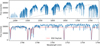 |
Fig. 1 Observed spectrum of the GJ 436 b system during mid-transit. Top panel: all 8 spectral orders. Due to heavy contamination by tellurics, we discard the bluest order shown as semi-transparent. Bottom panel: zoom-in on the reddest spectral order, compared with the telluric absorption model from the ESO SkyCalc tool (red). |
3 Data analysis
3.1 Model atmospheres
Models of the planet transmission spectra were created using petitRADTRANS (pRT, Mollière et al. 2019), which is a Python package for calculating transmission and emission spectra of exoplanets through radiative transfer. These model atmospheres are used as templates in our cross-correlation algorithm (see Sec. 3.2). We assumed a H2-He dominated atmosphere, which is required to explain the observed radius of the planet (Figueira et al. 2009; Nettelmann et al. 2010). For these species, Rayleigh scattering and collision induced absorption are included. Furthermore, we assume a temperature of 700 K (e.g., Turner et al. 2016). Since high-resolution transit spectroscopy mainly probes low pressures and is less sensitive to absolute abundances or changes in the pressure-temperature profile, using isothermal profiles is a sufficient approximation. Clouds are modeled using the gray cloud deck implementation from pRT.
In order to investigate the presence of different molecules, we created separate templates for H2O, CH4 and CO using the main isotopolog default line lists from the HITEMP database (Rothman et al. 2010; Hargreaves et al. 2020). Assuming a solar C/O ratio of 0.55 (e.g., Asplund et al. 2009), the abundances of these molecules and the mean molecular weight (MMW) were calculated using pRT’s poor_mans_nonequ_chem subpackage, which interpolates the abundances of prominent species from a chemical equilibrium table. For each of these molecular species, we generated a grid of templates with varying metallicities, ranging from solar to 1000× solar, and cloud deck altitudes, ranging from 0.1 mbar to 1 bar, spaced evenly on a log-scale, resulting in a total of 399 templates for each species. With this, we aim to place constraints on the metallicity of the atmosphere and examine the presence of a potential high altitude cloud deck, as suggested by Knutson et al. (2014).
Figure 3 shows some examples of our H2O templates generated with pRT to illustrate the effects of varying cloud deck pressures and metallicities, convolved to the spectral resolution of CRIRES+. As shown in the top panel, spectra with clouds at lower pressures (higher altitudes) have more muted spectral features, which decreases their detectability. The spectral features also become weaker at very low and very high metallicities, as shown in the bottom panel. This is because at higher metallicites, the scale height of the atmosphere is reduced resulting in effectively smaller signals, while at lower metallicities, the spectral features get covered by the continuum produced by clouds and/or collision induced absorption. Nevertheless, even in these cases, absorption lines are potentially detectable at the high spectral resolution with CRIRES+. The strongest H2O features can be seen in atmospheres with low-altitude or absent cloud decks with low to intermediate metallicites.
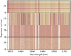 |
Fig. 2 Stages of data processing shown for the second spectral order. Top panel: observed spectra extracted from the CR2RES pipeline. Second panel: after masking of emission and absorption lines, continuum removal and outlier masking. Third panel: after removing the average off-transit spectrum. Bottom panel: after applying SYSREM. |
3.2 Detection pipeline
In our analysis, we make use of HRCCS for the detection of atmospheric species. The orbital parameters of GJ 436 b found in the literature are relatively consistent. For the most accurate ephemeris, we assumed the period P and transit midpoint T0 as determined by the Transiting Exoplanet Survey Satellite (TESS, Ricker et al. 2015). All of the parameters used in our analysis are listed in Table 1.
Our pipeline consists of several steps, conducted for each nodding position separately, and is based on that of Landman et al. (2021). Firstly, for each exposure and each spectral order, regions of the spectrum were masked where the flux is lower than 85% and higher than 120% of the normalized spectrum. This already removes a large fraction of emission and absorption lines caused by Earth’s atmosphere, as well as some deep stellar lines. The continuum was normalized for each order separately by fitting a third degree polynomial and dividing by it. Outliers at three times the standard deviation were masked. The result of these steps can be seen in the second panel of Fig. 2.
To correct for the still dominant telluric and stellar lines, each individual spectrum was divided by the average off-transit spectrum, with the result shown in the third panel of Fig. 2. While this removed most of the remaining contaminating features, some telluric and stellar residuals remained. Therefore, the de-trending algorithm SYSREM, designed to remove systematic effects in a large set of lightcurves (Tamuz et al. 2005; Mazeh et al. 2007), was subsequently applied to each order separately. It is based on principle component analysis (PCA), but unlike PCA, SYSREM also considers the individual errors of each data point. Dividing by the average off-transit spectrum beforehand decreased the runtime of SYSREM considerably. After four SYSREM iterations, as determined to maximize the S/N of injected model atmospheres, a final removal of outliers, at more than three times the standard deviation, was applied. The resulting spectra visually resemble pure noise, as they should at this stage of processing, and are shown in the bottom panel of Fig. 2.
Any potential planetary signal should be buried in the noise left over after removing the stellar and telluric features. Specific molecular species can now be searched for using cross-correlation with model spectra. Prior to cross-correlation, we Doppler-shifted the wavelengths of the data within a radial velocity range from −200 to +200 km s−1 with a step size of 1 km s−1, and linearly interpolated the template spectrum onto the shifted wavelength grid. The cross-correlation was computed by taking the inner product of the error-weighted observed spectra and the shifted template spectra. This results in a 2D map, showing the cross-correlation strength as function of radial velocity and planet orbital phase. A signal in the cross-correlation map at the expected radial velocity of the planet would indicate a detection.
The exoplanet’s radial velocity υp depending on its phase ϕ, as seen from Earth’s reference frame, can be calculated given its radial velocity semi-amplitude Kp, the barycentric velocity υbary caused by the Earth orbiting the barycenter of the Solar system, and the systemic velocity of the of the star–planet system υsys:
![Mathematical equation: $\[v_{\mathrm{p}}(\phi)=K_{\mathrm{p}} \cdot \sin (2 \pi \phi)-v_{\text {bary }}+v_{\text {sys}}.\]$](/articles/aa/full_html/2024/08/aa49932-24/aa49932-24-eq3.png) (1)
(1)
The barycentric velocity υbary is obtained from the time information of our data. The radial velocity semi-amplitude Kp is calculated using the semi-major axis a (derived from the planet mass Mp and stellar mass Ms), period P, eccentricity e and inclination i:
![Mathematical equation: $\[K_{\mathrm{p}}=\frac{2 \pi a}{P \sqrt{1-e^2}} \sin (i), \quad \text { with } a=\left(\frac{G \cdot\left(M_{\mathrm{s}}-M_{\mathrm{p}}\right) \cdot P^2}{4 \pi^2}\right)^{1 / 3} \text {. }\]$](/articles/aa/full_html/2024/08/aa49932-24/aa49932-24-eq4.png) (2)
(2)
The semi-amplitude of a circular orbit is Kp(e = 0) = Kp,c = 117.03 km s−1, while including the eccentricity results in a marginally larger value of Kp(e = 0.145) = Kp,e = 118.28 km s−1. However, accounting for the eccentricity only in Kp assumes the standard convention that the planetary argument of periastron is ωp = 270° at the middle of the transit (i.e., at an orbital phase of zero). Since GJ 436 b has an argument of periastron of ωp = 145.8°, the above equations are insufficient for describing the planet’s orbit accurately. For eccentric orbits, the value of ωp can have a profound impact on the orbital configuration and hence the radial velocity of the planet. Therefore, the eccentricity e, the planetary argument of periastron ωp and the true anomaly ν(ϕ) must be taken into account (e.g., Wright & Howard 2009; Basilicata et al. 2024) when calculating the planet’s radial velocity υp:
![Mathematical equation: $\[v_{\mathrm{p}}(\phi)=K_{\mathrm{p}} \cdot\left[\cos \left(\nu(\phi)+\omega_{\mathrm{p}}\right)+e \cdot \cos \left(\omega_{\mathrm{p}}\right)\right]-v_{\text {bary }}+v_{\text {sys}}.\]$](/articles/aa/full_html/2024/08/aa49932-24/aa49932-24-eq5.png) (3)
(3)
We used the python package “kepler.py2” to derive the true anomaly ν(ϕ) as a function of the phase, based on the planetary argument of periastron. To highlight the impact of the eccentricity on υp, we calculated the planet’s radial velocity for a circular (Eqs. (1) and (2) with e = 0) and eccentric (Eqs. (3) and (2) with e = 0.145) orbit for a direct comparison, as shown in Fig. 4.
To combine the signals from all in-transit observations, the cross-correlation functions (CCFs) were shifted to the rest frame of the GJ 436 system for each in-transit exposure and were summed. The CCFs were shifted according to the radial velocity from Eq. (1) using Kp values ranging from −250 to +350 km s−1, to check if the strongest signal appears at the expected Kp. The value of Kp reflects the radial velocity change during the transit, but due to the distortion of the orbit through the eccentricity, the effective Kp,eff for the eccentric orbit is not identical to Kp(e = 0.145) = Kp,e as calculated through Eq. (2). Instead, it is determined through the circular Kp,c (from Eq. (2) with e = 0) and the ratio of radial velocity change for the eccentric (Δυp,e) and circular (Δυp,c) orbit during the transit:
![Mathematical equation: $\[\frac{K_{\mathrm{p}, \mathrm{eff}}}{K_{\mathrm{p}, \mathrm{c}}}=\frac{\Delta v_{\mathrm{p}, \mathrm{e}}}{\Delta v_{\mathrm{p}, \mathrm{c}}}.\]$](/articles/aa/full_html/2024/08/aa49932-24/aa49932-24-eq6.png) (4)
(4)
The equation above results in an effective semi-amplitude of Kp,eff = 102.25 km s−1, which is where one would expect to find a planetary signal in the case of a detection. All steps until this point were run for both nodding positions, but now combined to increase any potential signal. The S/N of the cross-correlation peak was estimated by dividing the signal by the standard deviation, which was calculated excluding the velocity region of ±40 km s−1 around the a system rest frame velocity of zero, where one would expect the signal to be in the case of a circular orbit, and slightly shifted in the case of an eccentric orbit.
Our detection pipeline was calibrated by injecting a model spectrum at the planet’s radial velocity into the in-transit exposures. For this, we used a H2O template with a solar metallicity and cloud deck at 10 mbar. The S/N of the injected model was determined by running the pipeline with and without the injection and subsequently taking the difference of the CCFs, which we then divided by the standard deviation of the non-injected run. As such, the model spectrum’s retrieved S/N is the resulting value at the planet’s rest frame velocity and Kp. Through this process, we obtained the above mentioned optimum of four SYSREM iterations and removal of outliers at a standard deviation larger than three. In this way, we also found that employing a weighting scheme for the different orders based on the recovered S/N of the injected model does not lead to a higher S/N when removing the telluric-dominated orders from the analysis. In fact, only discarding the three most telluric-dominated orders without weighting produced the highest S/N of the recovered injected signal. Therefore, we constructed our pipeline accordingly. Both nodding positions yielded similar results.
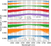 |
Fig. 3 Examples of H2O model atmospheres created with petitRADTRANS (Mollière et al. 2019). For clarity, an offset is added to the transit depth. The shaded regions illustrate the spectral coverage of CRIRES+. Top panel: 10× solar metallicity with varying cloud deck pressures. Bottom panel: cloud deck at 10 mbar with varying metallicities, with Z = 1 indicating a solar metallicity. |
Parameters of the GJ 436 system used in our analysis.
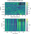 |
Fig. 4 Cross-correlation strength from the H2O template with a cloud deck at 10 mbar and 10× solar metallicity, summed over all spectral orders and both nodding positions. Top panel: CCFs for each spectrum, with the radial velocity in Earth’s rest frame on the x-axis and the transit phase and corresponding exposure number on the y-axes. The horizontal dashed lines indicate the beginning and end of the transit, while the slanted lines (circular orbit in white, true eccentric orbit in pink) shows the radial velocity of the planet during its transit and hence the expected location of the signal. Bottom panel: estimated S/N as a function of the planetary rest-frame velocity υsys and radial velocity semi-amplitude Kp. The intersection of the vertical and horizontal dashed lines (circular orbit in white, true eccentric orbit in pink) indicate the location of the expected signal in the absence of atmospheric winds. The pink ellipse encompasses the Kp and radial velocity values when considering the 1-σ errors of ωp, e, and Ms. |
4 Results
The detection pipeline was run using the generated H2O, CH4, and CO model atmospheres as templates for the cross-correlation. No signal was detected from any of these molecules in the data. Cross-correlating with OH and NH3 model atmospheres also resulted in non-detections.
As an example, we show the cross-correlation results from the H2O template with a cloud deck at 10 mbar and 10× solar metallicity. The top panel of Fig. 4 shows the cross-correlation strength for each spectrum (both nodding positions combined), summed over all spectral orders, as a function of the radial velocity and transit phase. The transit occurs between the horizontal dashed lines. The expected location of the planetary signal, assuming the true eccentric orbit or a circular orbit, are shown by slanted lines in pink and white, respectively. Accounting for the altered orbital configuration due to the eccentricity results in a significantly different radial velocity of the planet during its transit, shifted by an average of −14.3 km s−1 with respect to the circular orbit. The slope of the lines also differ slightly, reflecting a change in Kp from Kp,c = 117.03 km s−1 (circular) to Kp,eff = 102.25 km s−1 (effective eccentric). This highlights the need for accurate orbital calculations, which incorporate the eccentricity and argument of periastron, in studies that depend on the planet’s radial velocity. Precise values of these parameters are crucial for a correct orbital solution, as explored for instance by Basilicata et al. (2024). Failing to account for the effect of the eccentricity can, at best, partially smear the planetary signal, and at worst, shift it to completely different values and hinder a potential detection.
The bottom panel of Fig. 4 shows the estimated S/N derived from the CCFs, representing the detection significance, as a function of the system rest-frame velocity υsys and radial velocity semi-amplitude Kp. The intersection of the dashed lines show the expected location for the true eccentric orbit (pink) and circular orbit (white). In the rest-frame of the star, a planet on a circular orbit would have a radial velocity of zero during the transit, hence the position of the circular orbit at υsys = 0 km s−1 and at Kp,c = 117.03 km s−1. In contrast, the eccentric orbit of the planet leads to a shifted position in the Kp − υsys diagram at υsys = −14.3 km s−1 and at Kp,eff = 102.25 km s−1. In the case of a detection, a signal would appear where the pink lines intersect. No signal is detected at the expected location or anywhere else in the examined velocity range. In order to assess the impact of parameter uncertainties on Kp,eff and υp, we drew 1000 random values for e, ωp, and Ms from a uniform distribution of spanning ±1σ, from which we calculated Kp,eff and υp. The resulting range is highlighted by the pink ellipse. We conclude that the effect of the uncertainties is not too large, affecting Kp,eff by roughly ±4 km s−1 and υp by ±5 km s−1.
We use the data to constrain the atmospheric composition of GJ 436 b by determining the retrievability of various injected model atmospheres. For this, we use our previously generated grid of H2O, CH4, and CO templates with varying metallicities, ranging from solar to 1000 times solar, and cloud deck altitudes, ranging from 0.1 mbar to 1 bar. We ran our pipeline on each injected model atmosphere and determined the resulting S/N.
Figure 5 shows a 2d map of the retrieved S/N of the injected models for H2O (left), CH4 (middle), and CO (right) depending on metallicity and pressure. We highlight the contours of S /N = 3 and S /N = 5, and consider the latter as a detection threshold. For a comparison with the constraints from the HST data, the 99.7% posterior probability density from Fig. 3 in Knutson et al. (2014) is included. Due to the unavailability of the contour source data, these values were extracted from their figure using WebPlotDigitizer (Version 4.6, Rohatgi 2022).
Any injected model atmosphere with a recovered S/N > 5, as shown in Fig. 5, can be considered a detection, and can be ruled out as a possible atmosphere of GJ 436 b. Due to the highest achievable S/N, if present, H2O should be the most readily detectable molecule in this data. This is unsurprising, given the considerably larger transmission signal produced by H2O compared to CH4 and CO. Furthermore, in the wavelength range covered by CRIRES+, CO spectral features are only present in a very narrow range. Similarly, OH only has a few strong spectral lines in our considered wavelength range, while NH3 produces only a relatively small transmission signal.
Given our non-detection, we can rule out atmospheres in the bottom left corner of the H2O plot in Fig. 5, that is, atmospheres with low-altitude cloud decks (P > 10 mbar) and simultaneous solar to 300× solar metallicities. Our analysis indicates that the most likely scenario for GJ 436 b is a high-altitude cloud deck (P < 10 mbar) and/or a high metallicity (>300× solar), since it falls beyond the scope of what is detectable with the data. Given the planet radius and mass, a solar metallicity is less likely, but intermediate metallicities are expected (Figueira et al. 2009).
Figure 6 shows slices from Fig. 5 for selected metallicities (top row) and cloud decks (bottom row). In the case of all three molecules, a cloud deck at high pressures, and hence low altitudes, enhances the retrieved S/N, as seen in the top row of Fig. 6. Atmospheres with cloud decks at very low altitudes and hence high pressures are equivalent to cloud-free atmospheres. However, the effect of metallicity varies depending on the examined molecule, as seen in the bottom row of Fig. 6. The metallicity of an atmosphere can impact the retrieved S/N in two ways. For one, an atmosphere with a higher metallicity can increase the S/N due to containing more of the targeted molecules, which together produce stronger spectral features that are more prominent with respect to the continuum. On the other hand, a larger fraction of heavy elements also decreases the scale height of the atmosphere, which has the opposite effect.
Atmospheres in chemical equilibrium with temperatures like that of GJ 436 b are expected to contain H2O and CH4 due to their favored formation pathways, governed mainly by the reaction CO+3H2 ⇌ CH4+H2O. At lower temperatures and higher pressures, the equilibrium shifts towards the formation of CH4 (Seager 2010). However, as cross-correlation is considerably more sensitive to line positions than their depths and hence absolute absolute abundances, a higher S/N does not necessarily reflect a higher abundance and may instead be due to the higher number and density of lines in the probed wavelength region, resulting in a higher correlation peak. This can be seen in Fig. 5, where the higher obtainable S/N of the H2O signal arises due to its denser forest of lines in the H-band, while the relatively few spectral features of CO account for the lower S/N.
For H2O, a 10× solar metallicity produces the highest S/N. In Fig. 6, one can also see that for higher metallicities the S/N remains flat over a larger range of cloud deck altitudes. This is because the signal is mainly coming from higher in the atmosphere, so the cloud deck only starts to dampen the signal once it is at high altitudes. For CH4, a solar metallicity produces the highest S/N, while for CO, the highest S/N is achieved at about 50× solar metallicity. In our model atmospheres, assuming chemical equilibrium, the mass fractions of CH4 and CO both peak for higher metallicities (100–1000× solar), but this does not reflect in the retrieved S/N of the injected signals, as cross-correlation is not very sensitive to absolute abundances. For CH4, with prominent spectral features throughout our probed wavelength range, the decreasing scale height with higher metallicities appears to be producing the largest effect on its detectability. In contrast, the spectral features of CO are only present in a very narrow wavelength range and much less prominent with respect to the continuum at very high or low metallicities. Despite our non-detections, the presence of these molecules in GJ 436b’s atmosphere cannot be ruled out and requires further investigations.
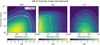 |
Fig. 5 Retrieved S/N of the injected model atmospheres for H2O (left), CH4 (middle), and CO (right) with varying metallicites and cloud deck altitudes. The white dashed lines indicate the contours for S/N = 3 and S/N = 5, with the latter taken as a detection threshold. The pink dotted curve (labeled as K14-3σ) is the 99.7% constraint from Fig. 3 in Knutson et al. (2014). |
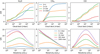 |
Fig. 6 Retrieved S/N of injected model atmospheres for H2O (left column), CH4 (middle column), and CO (right column), showing slices of selected metallicities Z (top row) and cloud deck altitudes (bottom row) from Fig. 5. |
5 Discussion
Our results are consistent with the flat transmission spectrum found by Knutson et al. (2014), produced either by high-altitude clouds and/or a high atmospheric metallicity. Assuming Gaussian noise properties (e.g., S/N = 3 is comparable to a probability of 99.7%), we compare the upper limits from Fig. 5 to the constraints shown in their Fig. 3, which are derived from four transits of HST data. Comparing our constraints from the S/N to the posterior probability density of Knutson et al. (2014) is of course a simplified approach and only serves as an approximation. However, since we only deal with injected signals, for which we know the position and line-shape exactly, this significantly reduces any biases.
The highlighted contours in Fig. 5 show that the 3σ constraints derived by Knutson et al. (2014) fall between our S/N = 3 and S/N = 5 limits. Consequently, for a given metallicity and cloud deck pressure, we estimate that CRIRES+ data would provide a somewhat higher S/N. From this, we postulate that one transit with CRIRES+ can offer constraints of slightly better or similar quality compared to four transits with HST. Furthermore, our findings also agree with other modeling and observational studies (Lanotte et al. 2014; Agúndez et al. 2014; Morley et al. 2017; Lothringer et al. 2018) that are compatible with a high-metallicity atmosphere.
The detection of H2O may be impeded by Earth’s telluric absorption, which overlaps with some strong H2O spectral features, in particular around 1400 nm. In the case of cloudy atmospheres, the signal from above the clouds comes mainly from the wavelength regions that also harbor strong telluric features. The fact that GJ 436 is an M-dwarf which also has H2O features further complicates the detection. The planet’s small radial velocity change during the transit makes it more difficult to disentangle its H2O features from those of the star.
Our non-detection is probably mainly due to the fact that we only obtained good quality data from one observing night. An additional two to three transits of high S/N might be sufficient for a detection, assuming that the S/N increases with the square root of the number of observations. The required number of transits for detection of a certain atmosphere can be estimated based on the S/N of the retrieved injected signals in Fig. 5. Given that we would obtain a S/N ~ 3 for a 10–100× solar metallicity atmosphere with a cloud deck at 1 mbar, only three observations of similar high quality would be required to reach a detection threshold of S/N ~ 5. Similarly, we would detect a high-metallicity atmosphere (1000× solar) with a low-altitude cloud deck (P > 100 mbar) at a S/N ~ 2.5, so only four high quality transits would be required to reach S/N ~ 5. Only the detection of high-metallicity atmospheres together with a high-altitude cloud deck would require an unfeasible amount of transits with CRIRES+, such as 40 transits for a 1000× solar metallicity and cloud deck at 1 mbar. In this regard, despite the promising potential of HRCCS for characterizing exoplanet atmospheres and higher sensitivity compared to HST, the combination of several high-quality observing nights may be required in the case of cloudy and/or high metallicity atmospheres.
Gandhi et al. (2020) predicted that HRS on 4m class telescopes, such as SPIRou, CARMENES or GIANO, could partially break the degeneracy between high metallicities and high-altitude clouds using 10 h of transit observations, which amounts to 10 transits in total given the planet’s 1 h transit duration. A direct comparison with their study is difficult due to significant methodological differences. For one, they deal with other instruments, which have a larger and more continuous wavelength coverage than CRIRES+, but are on smaller telescopes. Considering our above extrapolation from the S/N of injected model atmospheres, which shows that only four high quality transits would be required for a S/N ~ 5, combined with a twice as large telescope diameter, our findings appear to be more or less consistent with the predictions by Gandhi et al. (2020).
Alternatively, observations with other facilities also hold potential, such as the near-infrared spectrometer (NIRSpec) on the James Webb Space Telescope (JWST). Constantinou & Madhusudhan (2022) find that single-transit transmission spectra combining all three NIRSpec gratings can constrain H2O, CH4, and NH3 of the two temperate mini-Neptunes K2-18b and TOI-732c, for cloud deck pressures as low as 3 and 0.1 mbar, respectively, in the case of a 10× solar metallicity. In fact, the potential of JWST for characterizing sub-Neptunes is already being demonstrated by unprecedented findings, such as the detections of CH4 and CO2 in the mini-Neptune K2-18b (Madhusudhan et al. 2023) and in the sub-Neptune TOI-270d (Holmberg & Madhusudhan 2024). However, the transmission spectrum of the sub-Neptune TOI-836c also appears to be featureless with JWST data (Wallack et al. 2024).
6 Conclusion
We have obtained new high-resolution CRIRES+ observations of the warm Neptune GJ 436b. Cross-correlating the data with H2O, CH4, and CO model atmospheres of various metallicities and cloud deck altitudes yields a non-detection. Through injecting model atmospheres into the data and determining their retrievability, a range of atmospheric compositions can be ruled out, such as low to intermediate metallicities combined with a low-altitude cloud deck or a cloud-free atmosphere. Our analysis agrees with previous findings that the atmosphere of GJ 436 b most likely has a high-altitude cloud deck (P < 10 mbar) and/or a high-metallicity (>300× solar). Finally, a comparison of our detection thresholds with those derived from HST data (Knutson et al. 2014) appear to yield slightly better constraints. Therefore, we estimate that one transit with CRIRES+ may be somewhat higher in quality compared to four transits with HST. While this illustrates the promising potential of CRIRES+ spectroscopy for characterizing exoplanet atmospheres, the combination of at least several high S/N transits will be necessary for the detection of chemical species in cloudy and/or high metallicity atmospheres such as that of GJ 436 b.
Acknowledgements
We extend our gratitude to the anonymous referee, whose constructive feedback has significantly helped improve our paper. N.G. also wishes to thank M. Basilicata for the very helpful explanations about calculating eccentric orbits. Support for this work was provided by NL-NWO Spinoza SPI.2022.004. Our work is based on observations collected at the European Organisation for Astronomical Research in the Southern Hemisphere under ESO programme 110.2492.004. D.G.P acknowledges support from NWO grant OCENW.M.21.010.
References
- Agúndez, M., Venot, O., Selsis, F., & Iro, N. 2014, ApJ, 781, 68 [Google Scholar]
- Asplund, M., Grevesse, N., Sauval, A. J., & Scott, P. 2009, ARA&A, 47, 481 [NASA ADS] [CrossRef] [Google Scholar]
- Baluev, R. V., Sokov, E. N., Shaidulin, V. S., et al. 2015, MNRAS, 450, 3101 [Google Scholar]
- Basilicata, M., Giacobbe, P., Bonomo, A. S., et al. 2024, A&A, 686, A127 [NASA ADS] [CrossRef] [EDP Sciences] [Google Scholar]
- Batalha, N. M., Rowe, J. F., Bryson, S. T., et al. 2013, ApJS, 204, 24 [Google Scholar]
- Bean, J. L., Miller-Ricci Kempton, E., & Homeier, D. 2010, Nature, 468, 669 [NASA ADS] [CrossRef] [Google Scholar]
- Bean, J. L., Raymond, S. N., & Owen, J. E. 2021, J. Geophys. Res. Planets, 126, e06639 [NASA ADS] [CrossRef] [Google Scholar]
- Benneke, B., Roy, P.-A., Coulombe, L.-P., et al. 2024, arXiv e-prints [arXiv:2403.03325] [Google Scholar]
- Birkby, J. L., de Kok, R. J., Brogi, M., Schwarz, H., & Snellen, I. A. G. 2017, AJ, 153, 138 [NASA ADS] [CrossRef] [Google Scholar]
- Borucki, W. J., Koch, D. G., Basri, G., et al. 2011, ApJ, 736, 19 [Google Scholar]
- Bourrier, V., Lovis, C., Beust, H., et al. 2018, Nature, 553, 477 [NASA ADS] [CrossRef] [Google Scholar]
- Brogi, M., Snellen, I. A. G., de Kok, R. J., et al. 2012, Nature, 486, 502 [Google Scholar]
- Brogi, M., de Kok, R. J., Albrecht, S., et al. 2016, ApJ, 817, 106 [Google Scholar]
- Butler, R. P., Vogt, S. S., Marcy, G. W., et al. 2004, ApJ, 617, 580 [NASA ADS] [CrossRef] [Google Scholar]
- Constantinou, S., & Madhusudhan, N. 2022, MNRAS, 514, 2073 [NASA ADS] [CrossRef] [Google Scholar]
- Dorn, R. J., Anglada-Escude, G., Baade, D., et al. 2014, The Messenger, 156, 7 [NASA ADS] [Google Scholar]
- Ehrenreich, D., Bonfils, X., Lovis, C., et al. 2014, A&A, 570, A89 [NASA ADS] [CrossRef] [EDP Sciences] [Google Scholar]
- Ehrenreich, D., Bourrier, V., Wheatley, P. J., et al. 2015, Nature, 522, 459 [Google Scholar]
- Ehrenreich, D., Lovis, C., Allart, R., et al. 2020, Nature, 580, 597 [Google Scholar]
- Elkins-Tanton, L. T., & Seager, S. 2008, ApJ, 685, 1237 [NASA ADS] [CrossRef] [Google Scholar]
- Figueira, P., Pont, F., Mordasini, C., et al. 2009, A&A, 493, 671 [NASA ADS] [CrossRef] [EDP Sciences] [Google Scholar]
- Follert, R., Dorn, R. J., Oliva, E., et al. 2014, SPIE Conf. Ser., 9147, 914719 [Google Scholar]
- Fouqué, P., Moutou, C., Malo, L., et al. 2018, MNRAS, 475, 1960 [Google Scholar]
- Fressin, F., Torres, G., Charbonneau, D., et al. 2013, ApJ, 766, 81 [NASA ADS] [CrossRef] [Google Scholar]
- Gandhi, S., Brogi, M., & Webb, R. K. 2020, MNRAS, 498, 194 [Google Scholar]
- Gillon, M., Pont, F., Demory, B. O., et al. 2007, A&A, 472, L13 [NASA ADS] [CrossRef] [EDP Sciences] [Google Scholar]
- Hargreaves, R. J., Gordon, I. E., Rey, M., et al. 2020, ApJS, 247, 55 [NASA ADS] [CrossRef] [Google Scholar]
- Hoeijmakers, H. J., Cabot, S. H. C., Zhao, L., et al. 2020, A&A, 641, A120 [EDP Sciences] [Google Scholar]
- Holmberg, M., & Madhusudhan, N. 2024, A&A, 683, L2 [NASA ADS] [CrossRef] [EDP Sciences] [Google Scholar]
- Hood, C. E., Fortney, J. J., Line, M. R., et al. 2020, AJ, 160, 198 [NASA ADS] [CrossRef] [Google Scholar]
- Howard, A. W., Marcy, G. W., Bryson, S. T., et al. 2012, ApJS, 201, 15 [Google Scholar]
- Hu, R., Seager, S., & Yung, Y. L. 2015, ApJ, 807, 8 [Google Scholar]
- Jones, A., Noll, S., Kausch, W., Szyszka, C., & Kimeswenger, S. 2013, A&A, 560, A91 [NASA ADS] [CrossRef] [EDP Sciences] [Google Scholar]
- Kaeufl, H.-U., Ballester, P., Biereichel, P., et al. 2004, SPIE Conf. Ser., 5492, 1218 [NASA ADS] [Google Scholar]
- Kesseli, A. Y., Snellen, I. A. G., Alonso-Floriano, F. J., Mollière, P., & Serindag, D. B. 2020, AJ, 160, 228 [NASA ADS] [CrossRef] [Google Scholar]
- Knutson, H. A., Benneke, B., Deming, D., & Homeier, D. 2014, Nature, 505, 66 [Google Scholar]
- Kreidberg, L., Bean, J. L., Désert, J.-M., et al. 2014, Nature, 505, 69 [Google Scholar]
- Landman, R., Sánchez-López, A., Mollière, P., et al. 2021, A&A, 656, A119 [NASA ADS] [CrossRef] [EDP Sciences] [Google Scholar]
- Landman, R., Stolker, T., Snellen, I. A. G., et al. 2024, A&A, 682, A48 [NASA ADS] [CrossRef] [EDP Sciences] [Google Scholar]
- Lanotte, A. A., Gillon, M., Demory, B. O., et al. 2014, A&A, 572, A73 [NASA ADS] [CrossRef] [EDP Sciences] [Google Scholar]
- Line, M. R., Vasisht, G., Chen, P., Angerhausen, D., & Yung, Y. L. 2011, ApJ, 738, 32 [NASA ADS] [CrossRef] [Google Scholar]
- Lothringer, J. D., Benneke, B., Crossfield, I. J. M., et al. 2018, AJ, 155, 66 [NASA ADS] [CrossRef] [Google Scholar]
- Madhusudhan, N. 2012, ApJ, 758, 36 [NASA ADS] [CrossRef] [Google Scholar]
- Madhusudhan, N., & Seager, S. 2011, ApJ, 729, 41 [Google Scholar]
- Madhusudhan, N., Sarkar, S., Constantinou, S., et al. 2023, ApJ, 956, L13 [NASA ADS] [CrossRef] [Google Scholar]
- Mayor, M., Marmier, M., Lovis, C., et al. 2011, A&A submitted [arXiv:1109.2497] [Google Scholar]
- Mazeh, T., Tamuz, O., & Zucker, S. 2007, ASP Conf. Ser., 366, 119 [Google Scholar]
- Miller-Ricci, E., & Fortney, J. J. 2010, ApJ, 716, L74 [NASA ADS] [CrossRef] [Google Scholar]
- Mollière, P., Wardenier, J. P., van Boekel, R., et al. 2019, A&A, 627, A67 [Google Scholar]
- Morley, C. V., Knutson, H., Line, M., et al. 2017, AJ, 153, 86 [NASA ADS] [CrossRef] [Google Scholar]
- Moses, J. I., Line, M. R., Visscher, C., et al. 2013, ApJ, 777, 34 [Google Scholar]
- Nettelmann, N., Kramm, U., Redmer, R., & Neuhäuser, R. 2010, A&A, 523, A26 [NASA ADS] [CrossRef] [EDP Sciences] [Google Scholar]
- Noll, S., Kausch, W., Barden, M., et al. 2012, A&A, 543, A92 [NASA ADS] [CrossRef] [EDP Sciences] [Google Scholar]
- Nortmann, L., Pallé, E., Salz, M., et al. 2018, Science, 362, 1388 [Google Scholar]
- Ricker, G. R., Winn, J. N., Vanderspek, R., et al. 2015, J. Astron. Telesc. Instrum. Syst., 1, 014003 [Google Scholar]
- Rohatgi, A. 2022, Webplotdigitizer: Version 4.6, https://automeris.io/WebPlotDigitizer [Google Scholar]
- Rosenthal, L. J., Fulton, B. J., Hirsch, L. A., et al. 2021, ApJS, 255, 8 [NASA ADS] [CrossRef] [Google Scholar]
- Rothman, L. S., Gordon, I. E., Barber, R. J., et al. 2010, J. Quant. Spectrosc. Radiat. Transf., 111, 2139 [NASA ADS] [CrossRef] [Google Scholar]
- Rumenskikh, M. S., Khodachenko, M. L., Shaikhislamov, I. F., et al. 2023, MNRAS, 526, 4120 [NASA ADS] [Google Scholar]
- Seager, S. 2010, Exoplanet Atmospheres: Physical Processes (Princeton: Princeton University Press) [Google Scholar]
- Snellen, I. A. G., de Kok, R. J., de Mooij, E. J. W., & Albrecht, S. 2010, Nature, 465, 1049 [Google Scholar]
- Stevenson, K. B., Harrington, J., Nymeyer, S., et al. 2010, Nature, 464, 1161 [NASA ADS] [CrossRef] [Google Scholar]
- Stolker, T., & Landman, R. 2023, Astrophysics Source Code Library [record ascl:2307.040] [Google Scholar]
- Tamuz, O., Mazeh, T., & Zucker, S. 2005, MNRAS, 356, 1466 [Google Scholar]
- Torres, G., Winn, J. N., & Holman, M. J. 2008, ApJ, 677, 1324 [Google Scholar]
- Trifonov, T., Kürster, M., Zechmeister, M., et al. 2018, A&A, 609, A117 [NASA ADS] [CrossRef] [EDP Sciences] [Google Scholar]
- Turner, J. D., Pearson, K. A., Biddle, L. I., et al. 2016, MNRAS, 459, 789 [NASA ADS] [CrossRef] [Google Scholar]
- Wallack, N. L., Batalha, N. E., Alderson, L., et al. 2024, AJ submitted [arXiv:2404.01264] [Google Scholar]
- Wright, J. T., & Howard, A. W. 2009, ApJS, 182, 205 [Google Scholar]
All Tables
All Figures
|
Fig. 1 Observed spectrum of the GJ 436 b system during mid-transit. Top panel: all 8 spectral orders. Due to heavy contamination by tellurics, we discard the bluest order shown as semi-transparent. Bottom panel: zoom-in on the reddest spectral order, compared with the telluric absorption model from the ESO SkyCalc tool (red). |
| In the text | |
|
Fig. 2 Stages of data processing shown for the second spectral order. Top panel: observed spectra extracted from the CR2RES pipeline. Second panel: after masking of emission and absorption lines, continuum removal and outlier masking. Third panel: after removing the average off-transit spectrum. Bottom panel: after applying SYSREM. |
| In the text | |
|
Fig. 3 Examples of H2O model atmospheres created with petitRADTRANS (Mollière et al. 2019). For clarity, an offset is added to the transit depth. The shaded regions illustrate the spectral coverage of CRIRES+. Top panel: 10× solar metallicity with varying cloud deck pressures. Bottom panel: cloud deck at 10 mbar with varying metallicities, with Z = 1 indicating a solar metallicity. |
| In the text | |
|
Fig. 4 Cross-correlation strength from the H2O template with a cloud deck at 10 mbar and 10× solar metallicity, summed over all spectral orders and both nodding positions. Top panel: CCFs for each spectrum, with the radial velocity in Earth’s rest frame on the x-axis and the transit phase and corresponding exposure number on the y-axes. The horizontal dashed lines indicate the beginning and end of the transit, while the slanted lines (circular orbit in white, true eccentric orbit in pink) shows the radial velocity of the planet during its transit and hence the expected location of the signal. Bottom panel: estimated S/N as a function of the planetary rest-frame velocity υsys and radial velocity semi-amplitude Kp. The intersection of the vertical and horizontal dashed lines (circular orbit in white, true eccentric orbit in pink) indicate the location of the expected signal in the absence of atmospheric winds. The pink ellipse encompasses the Kp and radial velocity values when considering the 1-σ errors of ωp, e, and Ms. |
| In the text | |
|
Fig. 5 Retrieved S/N of the injected model atmospheres for H2O (left), CH4 (middle), and CO (right) with varying metallicites and cloud deck altitudes. The white dashed lines indicate the contours for S/N = 3 and S/N = 5, with the latter taken as a detection threshold. The pink dotted curve (labeled as K14-3σ) is the 99.7% constraint from Fig. 3 in Knutson et al. (2014). |
| In the text | |
|
Fig. 6 Retrieved S/N of injected model atmospheres for H2O (left column), CH4 (middle column), and CO (right column), showing slices of selected metallicities Z (top row) and cloud deck altitudes (bottom row) from Fig. 5. |
| In the text | |
Current usage metrics show cumulative count of Article Views (full-text article views including HTML views, PDF and ePub downloads, according to the available data) and Abstracts Views on Vision4Press platform.
Data correspond to usage on the plateform after 2015. The current usage metrics is available 48-96 hours after online publication and is updated daily on week days.
Initial download of the metrics may take a while.