| Issue |
A&A
Volume 688, August 2024
|
|
|---|---|---|
| Article Number | A170 | |
| Number of page(s) | 12 | |
| Section | Astrophysical processes | |
| DOI | https://doi.org/10.1051/0004-6361/202449318 | |
| Published online | 15 August 2024 | |
Discovery of a strong rotation of the X-ray polarization angle in the galactic burster GX 13+1
1
Department of Physics and Astronomy, 20014 University of Turku, Finland
e-mail: This email address is being protected from spambots. You need JavaScript enabled to view it.
2
INAF Istituto di Astrofisica e Planetologia Spaziali, Via del Fosso del Cavaliere 100, 00133 Roma, Italy
3
Dipartimento di Fisica, Università degli Studi di Roma “Tor Vergata”, Via della Ricerca Scientifica 1, 00133 Roma, Italy
4
Dipartimento di Fisica, Università degli Studi di Roma “La Sapienza”, Piazzale Aldo Moro 5, 00185 Roma, Italy
5
MIT Kavli Institute for Astrophysics and Space Research, Massachusetts Institute of Technology, 77 Massachusetts Avenue, Cambridge, MA 02139, USA
6
Serco for the European Space Agency (ESA), European Space Astronomy Centre, Camino Bajo del Castillo s/n, 28692 Villanueva de la Cañada, Madrid, Spain
7
Dipartimento di Matematica e Fisica, Università degli Studi Roma Tre, Via della Vasca Navale 84, 00146 Roma, Italy
8
Nordita, KTH Royal Institute of Technology and Stockholm University, Hannes Alfvéns väg 12, 106 91 Stockholm, Sweden
9
Anton Pannekoek Institute for Astronomy & GRAPPA, University of Amsterdam, Science Park 904, 1098 XH Amsterdam, The Netherlands
10
Centre for Extragalactic Astronomy, Department of Physics, Durham University, South Road, Durham DH1 3LE, UK
11
Kavli Institute for Physics and Mathematics of the Universe (WPI), University of Tokyo, Kashiwa, Chiba 277-8583, Japan
12
University of British Columbia, Vancouver, BC V6T 1Z4, Canada
13
NASA Marshall Space Flight Center, Huntsville, AL 35812, USA
14
Instituto de Astrofísica de Andalucía – CSIC, Glorieta de la Astronomía s/n, 18008 Granada, Spain
15
INAF Osservatorio Astronomico di Roma, Via Frascati 33, 00040 Monte Porzio Catone, (RM), Italy
16
Space Science Data Center, Agenzia Spaziale Italiana, Via del Politecnico snc, 00133 Roma, Italy
17
INAF Osservatorio Astronomico di Cagliari, Via della Scienza 5, 09047 Selargius (CA), Italy
18
Istituto Nazionale di Fisica Nucleare, Sezione di Pisa, Largo B. Pontecorvo 3, 56127 Pisa, Italy
19
Dipartimento di Fisica, Università di Pisa, Largo B. Pontecorvo 3, 56127 Pisa, Italy
20
Istituto Nazionale di Fisica Nucleare, Sezione di Torino, Via Pietro Giuria 1, 10125 Torino, Italy
21
Dipartimento di Fisica, Università degli Studi di Torino, Via Pietro Giuria 1, 10125 Torino, Italy
22
INAF Osservatorio Astrofisico di Arcetri, Largo Enrico Fermi 5, 50125 Firenze, Italy
23
Dipartimento di Fisica e Astronomia, Università degli Studi di Firenze, Via Sansone 1, 50019 Sesto Fiorentino (FI), Italy
24
Istituto Nazionale di Fisica Nucleare, Sezione di Firenze, Via Sansone 1, 50019 Sesto Fiorentino (FI), Italy
25
Agenzia Spaziale Italiana, Via del Politecnico snc, 00133 Roma, Italy
26
Science and Technology Institute, Universities Space Research Association, Huntsville, AL 35805, USA
27
Istituto Nazionale di Fisica Nucleare, Sezione di Roma “Tor Vergata”, Via della Ricerca Scientifica 1, 00133 Roma, Italy
28
Department of Physics and Kavli Institute for Particle Astrophysics and Cosmology, Stanford University, Stanford, California 94305, USA
29
Institut für Astronomie und Astrophysik, Universität Tübingen, Sand 1, 72076 Tübingen, Germany
30
Astronomical Institute of the Czech Academy of Sciences, Boční II 1401/1, 14100 Praha 4, Czech Republic
31
RIKEN Cluster for Pioneering Research, 2-1 Hirosawa, Wako, Saitama 351-0198, Japan
32
X-ray Astrophysics Laboratory, NASA Goddard Space Flight Center, Greenbelt, MD 20771, USA
33
Yamagata University, 1-4-12 Kojirakawa-machi, Yamagata-shi 990-8560, Japan
34
Osaka University, 1-1 Yamadaoka, Suita, Osaka 565-0871, Japan
35
International Center for Hadron Astrophysics, Chiba University, Chiba 263-8522, Japan
36
Institute for Astrophysical Research, Boston University, 725 Commonwealth Avenue, Boston, MA 02215, USA
37
Department of Astrophysics, St. Petersburg State University, Universitetsky pr. 28, Petrodvoretz, 198504 St. Petersburg, Russia
38
Department of Physics and Astronomy and Space Science Center, University of New Hampshire, Durham, NH 03824, USA
39
Physics Department and McDonnell Center for the Space Sciences, Washington University in St. Louis, St. Louis, MO 63130, USA
40
Istituto Nazionale di Fisica Nucleare, Sezione di Napoli, Strada Comunale Cinthia, 80126 Napoli, Italy
41
Université de Strasbourg, CNRS, Observatoire Astronomique de Strasbourg, UMR 7550, 67000 Strasbourg, France
42
Graduate School of Science, Division of Particle and Astrophysical Science, Nagoya University, Furo-cho, Chikusa-ku, Nagoya, Aichi 464-8602, Japan
43
Hiroshima Astrophysical Science Center, Hiroshima University, 1-3-1 Kagamiyama, Higashi-Hiroshima, Hiroshima 739-8526, Japan
44
Department of Physics and Astronomy, Louisiana State University, Baton Rouge, LA 70803, USA
45
Department of Physics, University of Hong Kong, Pokfulam, Hong Kong
46
Department of Astronomy and Astrophysics, Pennsylvania State University, University Park, PA 16801, USA
47
Université Grenoble Alpes, CNRS, IPAG, 38000 Grenoble, France
48
Center for Astrophysics, Harvard & Smithsonian, 60 Garden St, Cambridge, MA 02138, USA
49
INAF Osservatorio Astronomico di Brera, Via E. Bianchi 46, 23807 Merate (LC), Italy
50
Dipartimento di Fisica e Astronomia, Università degli Studi di Padova, Via Marzolo 8, 35131 Padova, Italy
51
Department of Astronomy, University of Maryland, College Park, Maryland 20742, USA
52
Mullard Space Science Laboratory, University College London, Holmbury St Mary, Dorking, Surrey RH5 6NT, UK
53
Guangxi Key Laboratory for Relativistic Astrophysics, School of Physical Science and Technology, Guangxi University, Nanning 530004, PR China
Received:
23
January
2024
Accepted:
3
May
2024
Abstract
Weakly magnetized neutron stars in X-ray binaries show a complex phenomenology with several spectral components that can be associated with the accretion disk, the boundary, and/or a spreading layer, a corona, and a wind. Spectroscopic information alone, however, is not enough to distinguish these components. The analysis of the timing data revealed that most of the variability, and in particular, kilohertz quasi-period oscillations, are associated with the high-energy component that corresponds to the boundary and/or spreading layer. Additional information about the nature of the spectral components, and in particular, about the geometry of the emission region, can be provided by X-ray polarimetry. One of the objects of the class, a bright, persistent, and rather peculiar galactic Type I X-ray burster GX 13+1, was observed with the Imaging X-ray Polarimetry Explorer (IXPE) and the XMM–Newton. Using the XMM–Newton data, we obtained the best-fit values for the continuum spectral parameters and detected strong absorption lines associated with the accretion disk wind. IXPE data showed the source to be significantly polarized in the 2–8 keV energy band, with an overall polarization degree (PD) of 1.4%±0.3% at a polarization angle (PA) of −2° ±6° (errors at the 68% confidence level). During the two-day long observation, we detected rotation of the PA by about 70° with the corresponding changes in the PD from 2% to nondetectable and then up to 5%. These variations in polarization properties are not accompanied by visible spectral state changes of the source. The energy-resolved polarimetric analysis showed a significant change in polarization, from being strongly dependent on energy at the beginning of the observation to being almost constant with energy in the later parts of the observation. As a possible interpretation, we suggest a constant polarization component, strong wind scattering, or a different polarization of the two main spectral components with an individually peculiar behavior. The rotation of the PA suggests a misalignment of the neutron star spin from the orbital axis.
Key words: accretion / accretion disks / polarization / stars: neutron / X-rays: binaries
© The Authors 2024
 Open Access article, published by EDP Sciences, under the terms of the Creative Commons Attribution License (https://creativecommons.org/licenses/by/4.0), which permits unrestricted use, distribution, and reproduction in any medium, provided the original work is properly cited.
This article is published in open access under the Subscribe to Open model. This email address is being protected from spambots. You need JavaScript enabled to view it. to support open access publication.
1. Introduction
Weakly magnetized neutron stars (WMNSs) reside in low-mass X-ray binary (LMXB) systems and accrete material from companion stars via an accretion disk. With their luminosity ranging in the 1036 − 1038 erg s−1, they are among the brightest X-ray sources in the sky. WMNSs can be classified as Z- or atoll-sources, based on the shape of their tracks in the X-ray hardness-intensity (HID) diagram or in the color-color diagram (CCD), their timing proprieties in the 1–10 keV band, their radio emission, and their luminosity and mass-accretion rate. WMNSs are also known for their fast X-ray variability: The quasi-periodic oscillations in the ranges seconds and milliseconds that were observed from many sources of the class (van der Klis 1989, 2000; Méndez & Belloni 2021) are associated with a harder spectral component (Gilfanov et al. 2003; Revnivtsev & Gilfanov 2006; Revnivtsev et al. 2013) close to the neutron star (NS) surface.
In the absence of a strong magnetic field surrounding the NS in these systems, the matter from the accretion disk falls onto the equator of the star via the boundary layer (BL, see e.g. Shakura & Sunyaev 1988) and further spreads throughout the NS surface, where it forms the so-called spreading layer (SL, see e.g. Lapidus & Sunyaev 1985; Inogamov & Sunyaev 1999). The geometry and physics of the processes that occur within these layers both affect the emission of WMNSs and their polarization (see e.g. Lapidus & Sunyaev 1985; Gnarini et al. 2022). The emission of WMNSs in the X-ray band has two main components: a soft thermal emission, which can be blackbody-like emission from the NS surface or a multicolor emission from the disk, and a harder component associated with the Comptonization in the BL or SL. In addition to these two main components, signs of reflection of the SL emission from the accretion disk (usually a broad emission line around 6.4 keV) and a set of absorption lines are sometimes visible, which indicates that the radiation interacts in the wind above the disk. A contribution of the hot corona is also possible, as is a contribution of the hot flow in the hard state.
Polarimetry is a useful tool for understanding the geometry of the source and the emission mechanisms by studying the two additional variables it provides: the polarization degree (PD), and polarization angle (PA). The Imaging X-ray Polarimetry Explorer (IXPE; Weisskopf et al. 2022), launched in December 2021, is a pathfinder that gives us the unique opportunity to measure the X-ray polarimetric properties of WMNSs with high precision. In the last two years, nine objects of the class were observed (see Capitanio et al. 2023; Farinelli et al. 2023; Cocchi et al. 2023; Ursini et al. 2023; Di Marco et al. 2023a; Rankin et al. 2024; La Monaca et al. 2024; Saade et al. 2024; Fabiani et al. 2024). These observations shed new light on the emission mechanisms of these sources, as well as on the changes in PD and PA while the source changes its spectral state. We aim to add another important piece of evidence to the global picture.
GX 13+1 is a peculiar source with a unique position between atolls and Z-sources. It is located at a distance of 7 ± 1 kpc in a binary system and has a late-evolved K5 III giant as a companion (Bandyopadhyay et al. 1999). The source shows several features that have traditionally been associated with Z-sources: It shines almost as brightly as Z-sources (up to 0.5LEdd, D’Aí et al. 2014), it has persistent radio emission (Grindlay & Seaquist 1986), and it shows 57–69 Hz quasi-periodic oscillations (Homan et al. 1998). The path it draws on the CCD, however, is closer to the path normally observed from the atolls (Schnerr et al. 2003). However, even the CCD of the source has recently been interpreted as if GX 13+1 were a Z-source (Saavedra et al. 2023; Allen et al. 2018). Another unique property of GX 13+1 is the complex spectrum (e.g., Díaz Trigo et al. 2012). In addition to the common softer accretion disk and harder Comptonized components, a sign of reflection of the Comptonized emission from the disk is present, as well as seven absorption features caused by the interaction of the radiation in the wind above the disk. Allen et al. (2018) showed that these absorption features could not be produced by a single absorbing region, which indicates a complicated structure of the wind. GX 13+1 also exhibits periodic variations in the emission with a period of 24.5 d (Corbet et al. 2010). These modulations are associated with the orbital movement of the source, making GX 13+1 the NS–LMXB with the longest orbital period. Short dips of ≈1 ks in the X-ray spectrum are associated with this orbital movement (Diaz Trigo et al. 2010; Iaria et al. 2014), but they are occasional events and are not present in every orbit. These dips are traditionally interpreted as an indication of the high source inclination (60° −75°). They come from the interaction of the emission of the NS with the mostly neutral accretion bulge located in the outer parts of the disk (White & Holt 1982; D’Aí et al. 2014).
The wind above the accretion disk of GX 13+1 has been studied with several observatories. For instance, using Chandra data, Tomaru et al. (2020) gave constraints on the radial and azimuthal velocity of the wind, and Allen et al. (2018) constrained the wind-launching radius, showing that the radiation pressure likely launches the wind. Maiolino et al. (2019) developed a nonrelativistic framework capable of fitting and interpreting the asymmetric Kα lines in XMM–Newton data and reported that this nonrelativistic approach performs as well as the known relativistic framework. This adds an alternative explanation of the red-skewed Fe line in the spectrum of GX 13+1. Saavedra et al. (2023) used NuSTAR data to estimate the distance between the source and the ionized absorbing material of (4 − 40)×105 km, constrained the magnetic field at B ≲ 1.8 × 10⁸ G, and pointed out the overabundance of Fe and Ni in the source. GX 13+1 is also in the list of targets for the recently launched X-ray Imaging and Spectroscopy Mission (XRISM; XRISM Science Team 2022). The aim of our project is to obtain constraints on the source geometry and radiation mechanisms using the polarimetric capabilities of IXPE.
The remainder of the paper is structured as follows. We introduce the observations performed with IXPE and the XMM–Newton observatories in Sect. 2. In Sect. 3 we present the data analysis. We provide an interpretation of the results in Sect. 4 and summarize in Sect. 5.
2. Observations
2.1. IXPE
The IXPE was launched on 2021 December 9 as a result of joint efforts of NASA and the Italian Space Agency. It has three identical grazing-incidence telescopes on board, each of which comprises an X-ray mirror assembly and a polarization-sensitive detector unit (DU) equipped with a gas-pixel detector (Soffitta et al. 2021; Baldini et al. 2021). IXPE is capable of performing imaging polarimetry over the 2–8 keV energy band with a time resolution of about 10 μs. A detailed description of the observatory and its performance is given in Weisskopf et al. (2022).
IXPE observed GX 13+1 on 2023 October 17–19 with a total effective exposure of ≃100 ks for each of the three telescopes (see Table 1). For the data analysis, we used the IXPEOBSSIM software, version 30.6.3 (Baldini et al. 2022), and the HEASOFT package, version 6.31.1 (NASA High Energy Astrophysics Science Archive Research Center (HEASARC)). We used the latest version of the IXPE response matrices, released at the HEASARC CALDB on 2023 June 16. We extracted the I, Q, and U spectra from a region with a radius of 80″. Following Di Marco et al. (2023b), we did not perform background subtraction or rejection, as GX 13+1 is sufficiently bright for the background to be negligible. The polarimetric analysis was performed using the formalism of Kislat et al. (2015) implemented in the IXPEOBSSIM package (Baldini et al. 2022) under the pcube algorithm in the xpbin tool. We used IXPEOBSSIM to investigate the time-dependence of the normalized Stokes parameters q = Q/I and u = U/I, as well as the PD and PA
 (see Figs. 1a–d). We applied the unweighted analysis implemented in the IXPEOBSSIM. For the spectral and spectropolarimetric analysis, we used XSPEC, version 12.13.0c (Arnaud 1996), and applied a weighted analysis as introduced in Di Marco et al. (2022). For the spectral analysis, the data were binned to have at least 30 counts in each energy bin. For the spectropolarimetric analysis, we applied a constant energy binning of 80 eV for the three Stokes parameters.
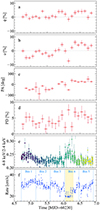 |
Fig. 1. Normalized Stokes q (a) and u (b) parameters, PA (c), PD (d), hardness ratio (e) with the same colors as in Fig. 2, and the count rate (f) as functions of time as observed by IXPE (all three detectors combined in the energy range 2–8 keV). The light curve is binned in ≈200 s. The dashed vertical blue lines separate the observation into five equal time bins of 10.5 h (Bins 1–5). The region highlighted in yellow corresponds to the dip in the light curve (see Sect. 3.1). Uncertainties are reported at the 68% CL. |
Observations of GX 13+1 presented in the paper.
2.2. XMM–Newton
XMM–Newton observed GX 13+1 on 2023 October 16 (see Table 1). This observation could not be scheduled simultaneously with IXPE because the visibility window for GX 13+1 with XMM–Newton closed on October 16. As GX 13+1 is very bright, EPIC/PN was operated in timing mode. The thick filter was used to reduce the count rate, which was about 690 cnt s−1 on average during the observation. The EPIC/MOS instruments were not used, and their telemetry was allocated to EPIC/PN. Despite this effort, PN nevertheless suffered from telemetry gaps as the science buffer was full throughout the observation. For this reason, the data are not suitable for a timing analysis, but are still useful for measuring the spectral shape and the known wind lines in the 6–9 keV range (Díaz Trigo et al. 2012).
The data were reduced using XMM–SAS v.21 with the latest calibration files as of October 2023. The clean event files were generated from the ODF files with the epchain tool. They were filtered further using the #XMMEA_EP and PATTERN==0 flags in the 0.3–12 keV range. No soft proton flares were seen in the light curves above 10 keV, giving us a total effective exposure of ≃10 ks. To extract the source spectrum, we selected events from a 9-pixel wide box around the RAWX column with the highest count rate. We also extracted a background spectrum from RAWX columns 3–5, but as expected for such a bright target, these columns were still dominated by the source itself, and thus, we did not subtract the background at all. The ancillary response file and the redistribution matrix were generated using the tools arfgen and rmfgen, respectively. Finally, we grouped the data to have at least 20 counts per channel and added 1% systematic errors in quadrature to each channel using the grppha tool.
3. Data analysis
3.1. Model-independent polarimetric analysis
The light curve of GX 13+1 is shown in Fig. 1f. The source showed some variations, with the count rate dropping by almost a factor of two in the wide dip, but some more rapid dips are noticeable. The hardness ratio (Fig. 1e) changes with time by only a small margin; the largest increase slightly after MJD 60236 coincides with the wide dip in the light curve and is ≈10%.
The significant variability of the Stokes parameters is immediately obvious. This variability is reflected in the changes in PD and PA in Figs. 1c,d. While the PA slowly increases throughout the observation, the PD changes significantly and without an obvious pattern.
The HID presented in Fig. 2 illustrates a lack of state variability within the more than two days of IXPE observation. From the data publicly available in the MAXI (Matsuoka et al. 2009) archive1 of the most recent observations, we calculated the CCD from the ratio of fluxes F10 − 20 keV/F4 − 10 keV against the ratio F4 − 10 keV/F2 − 4 keV. We then estimated the position of the points corresponding to the observation days on the CCD and concluded that the source during the IXPE observation was in the so-called lower left banana (LLB) state, a soft state common for the atoll sources. In the two days of IXPE observation, GX 13+1 moved in the lower left part of the CCD, but the uncertainties are too high to conclude about the state variability. Polarimetric analysis of the averaged data in the 2–8 keV energy band resulted in low PD values of 1.4%±0.3% and a PA of −2° ±6° (from here onward, the errors are given at the 68% confidence level, CL) with the significance of the detection exceeding 99.99% (see Fig. 3 and Table 2).
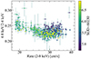 |
Fig. 2. Hardness-intensity diagram derived from the IXPE data in time bins of 200 s. The colors correspond to the evolution of the data with time, from dark blue at the beginning of the observation to yellow at the end of the observation. |
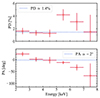 |
Fig. 3. Energy-resolved PD and PA averaged over all the IXPE observation, obtained with the pcube algorithm. The data are divided into six 1-keV wide energy bins. Uncertainties are reported at the 68% CL. |
Results of the pcube analysis performed with various approaches to separate the data.
As the HID does not show any significant change of state, we decided to perform a more detailed study of different parts of the observation based on the light curve. We separated the dip state (highlighted in yellow in Fig. 1f) from the nondip states and divided the observation into three unequal parts: the pre-dip (before t = 6.05 d), the dip (6.05 < t < 6.30 d), and the post-dip (t > 6.30 d), with the times t given relative to MJD 60230. The results are gathered in Fig. 4. The PD in the dip state is 2.2%±1.1%, and the PA is −49° ±14° at 68% CL. Due to the lack of statistics, we chose not to perform an energy-resolved analysis of this part of the observation.
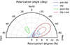 |
Fig. 4. Polar plot of the PD and PA in the 2–8 keV energy band for the three parts of the observation (pre-dip, dip, and post-dip) and the dip core. Contours are at the 68% CL (dashed lines) and 99% CL (solid lines). |
However, the pre- and post-dip parts show an interesting and completely different behavior (see Table 2). The energy-resolved PA and PD for these parts are presented in Fig. 5, and the corresponding Stokes q and u parameters are shown in Fig. 6. We also additionally studied the dip core, one specific bin in Fig. 1 at t = 6.15 d that falls out of the patterns in Figs. 1a and b. This bin lies in the middle of the hardening in Fig. 1e and of the dip in Fig. 1f, which makes it particularly interesting. As mentioned in Table 2, the PD there exceeds 7%, and the PA is below −50° with a significance of the detection higher than 99%.
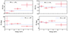 |
Fig. 5. Energy dependence of the PD and PA obtained by the pcube algorithm. Left: Pre-dip part of the observation. Right: Post-dip part of the observation. The data are divided into four energy bins: 2–3, 3–4, 4–5.5, and 5.5–8 keV. Uncertainties are reported at 68% CL. |
The change in PD behavior is noticeable. In the pre-dip part, the PD strongly depended on energy and increased from an upper limit of 1.7% at 2σ CL in the 2–3 keV bin to a strong detection of 5.5% in the 5.5–8 keV bin. In the post-dip part, however, the PD was almost constant with energy and averaged at about 5.3%, exceeding 7% in the 5.5–8 keV bin. No significant PA dependence on energy is observed in either part of the observation, but the value of the angle shifts by almost 60° between the pre-dip and post-dip parts. This complete change in the behavior between the two parts of the observation is also visible in the Stokes q − u plane (see Fig. 6): The polarization vector changes in amplitude and direction.
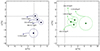 |
Fig. 6. Same as Fig. 5, but for the normalized Stokes parameters q and u. Arrows only indicate the label of the energy band. Uncertainties are reported at 68% CL. |
To study the separation of the observation in even more detail, we split it into five equal parts of 10.5 h each (bins 1–5 are defined with vertical dashed blue lines in Fig. 1f). The results are shown in Fig. 7 and Table 2. We performed a fit of the five PA values with a straight line (see Fig. 8) and confirmed the clear rotation of the PA with time with a slope of 1 64 per hour and a total rotation angle exceeding 70°. We also note that the PD is relatively high at the beginning and end of the observation. We note here that the polarization in bins 2, 3, and 4 in Fig. 7 is consistent with zero within the error bars at 99% CL. Thus, as three individual measurements, they are not significant, but as a part of the trend, they are still meaningful. The important conclusion we make here is that the dip does not fully cause the variability in the polarimetric properties. As can be concluded from the data presented in Table 2, the drop in PD already occurred in bin 2, while the dip occurs around bin 4. The PA rotates throughout the whole observation. The anomalies in the PA and PD occur around the time corresponding to the dip in the light curve in Fig. 1, but the general trend for PA and PD is not directly correlated with the dip.
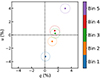 |
Fig. 7. Time dependence of the normalized Stokes parameters q and u obtained by the pcube algorithm using the data separation into five equal time bins. Uncertainties are reported at the 68% CL. |
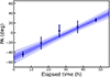 |
Fig. 8. Linear fit of the PA obtained for time bins 1–5 in Fig. 1f. The plot illustrates the rotation of the polarization plane with time. Uncertainties are reported at the 68% CL. |
Last but not least, we attempted to divide the observation into two parts by the count rate: below and above 25 cnt s−1. Data below the threshold fall into one of the many dips in the light curve. In the brighter state (above 25 cnt s−1), we saw a PD of ≈1.6% and PA of ≈2°, which is similar to that shown in Fig. 3 and in Table 2 for the overall polarization. The dimmer state (below 25 cnt s−1) showed PD ≈ 1.3% and PA ≈ −36°, which is in between the wide dip state of the previous analysis (between MJD−60230 = 6.05 and 6.30, as shown in Fig. 1f) and the overall polarization. Thus, adding the data obtained from the times corresponding to all the minor dips smoothed the difference between the anomalous polarimetric behavior during the dip and the general trend that we observed. It shifted the dimmer state PA and PD closer to the overall states than those of the wide dip. The polarimetric properties of the minor dips are then different from those of the wide dip, which means that the nature of the wide dip is different from the nature of all other dips in the light curve we observed.
3.2. Spectroscopic analysis
3.2.1. XMM–Newton
In the XMM–Newton data, below 2 keV, the count rate drops significantly due to the high interstellar absorption. We observe a significant excess below 2 keV with any continuum model combination. High residuals are also seen near the instrumental edges. In combination with our inability to subtract the background, this led us to discard these low-energy data. After all, they do not affect the modeling at higher energies.
Thus, we modeled the spectrum of the XMM–Newton observation in the 2–10 keV range. As we traditionally expect two continuum components to be present in the spectrum of a WMNS with some additional reflection and absorption features, we performed a fit with a tbabs*(diskbb+bbodyrad+gaussian) model modified by four Gaussian absorption lines, gabs, and two interstellar dust absorption edges, edge. The results are shown in Table 3 and in Fig. 9. To properly resolve the absorption features in the 6–9 keV energy range, we fixed the parameters of the gaussian corresponding to the broad emission line.
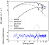 |
Fig. 9. Spectral energy distribution of GX 13+1 in EFE representation. The blue crosses show the data from XMM–Newton. The different spectral model components are reported as black lines for diskbb (short dashed), bbodyrad (long dashed), and gaussian (dotted). The total model is shown with a solid black line. The bottom panel shows the residuals between the data and the best fit. The data are rebinned only for plotting purposes. |
Best-fit parameters of GX 13+1 spectrum from XMM–Newton data.
The resulting fit illustrates that the spectrum of GX 13+1 is dominated by the disk. The harder component is modeled with the blackbody (as suggested in Schnerr et al. 2003; Díaz Trigo et al. 2012; Revnivtsev et al. 2013) and dominates at energies higher than 7 keV. Four strong absorption lines at 6.90, 7.18, 8.10, and 8.48 keV are also visible. These lines are identified with the Fe XXV Heα resonant line at 6.700 keV, Fe XXVI Lyα doublet at 6.966 keV, Ni XXVII Heα resonant line at 7.806 keV, and Ni XXVIII Lyα doublet at 8.092 keV, and they are well known in the source (see, e.g., Tomaru et al. 2020); three other known lines are not resolved in our fit. Compared with the previous results, the energies of the lines we obtain are higher than in Díaz Trigo et al. (2012) and correspond to a very high blueshift, z = −0.03 for the Fe lines and even higher for the Ni lines (although the latter are known to be blended with Fe Heβ lines) and might come from the full science buffer of the XMM–Newton during our observation. It is known that in this source, the wind is complex, very structured, and highly variable, and we therefore avoid interpreting this nominal blueshift without a much more detailed analysis of the absorption features, which is well beyond the scope of this paper. However, we do not expect this issue to significantly affect the continuum parameters in which we are mostly interested. We also note the anomalously high equivalent hydrogen column density parameter NH of the absorption component.
Additionally, we tried to model the XMM–Newton spectrum with only one continuum component. That is, we removed the bbodyrad component, and fit the whole continuum using a single diskbb component with high kTdbb ≈ 1.9 keV, resulting in a bad χ2/d.o.f.= 2058/1485 corresponding to a null-hypothesis probability < 10−3% with respect to the 34% achieved from the fit reported in Table 3.
3.2.2. IXPE
As the HID obtained from the IXPE data in Fig. 2 has rather large uncertainties and was obtained over a small energy range, it is not the most informative representation of the spectral variation in the data with time. We used XSPEC to fit the I spectrum obtained by IXPE. For this study, we chose the same five equal time bins as for the pcube analysis presented in Fig. 7. All five spectra were fit with the same model tbabs*(diskbb+bbodyrad). Considering the spectral capabilities of IXPE and the small effective area above 6 keV, we did not attempt to add the gabs or gaussian components that were prominent in the XMM–Newton spectrum. We multiplied the model by the constant component to scale the data from the three detectors of IXPE. We also fixed the value of the equivalent hydrogen column density NH, as IXPE does not have the capability to estimate it, and the temperature of the bbodyrad component to the best-fit values obtained with the XMM–Newton. We applied the weighted analysis introduced in Di Marco et al. (2023b). The results are presented in Table 4 and Fig. 10.
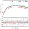 |
Fig. 10. Spectral energy distribution of the source in EFE representation during five equal parts of the observation. Here, only IXPE DU1 is reported as an example, and the data are rebinned for plotting purposes. |
Best-fit parameters of GX 13+1 spectrum from IXPE data divided into five equal time bins.
We note the lack of a change in the spectral parameters with time. The temperature of the disk does not vary with time, and only the normalization of the continuum components decreases toward the end of the observation, which could be consistent with increased absorption or scattering in the disk wind during the last part of the observation. In bin 5 of the observation, the contribution of the blackbody component also drops by a factor of two (however, the normalizations of all the blackbody components are compatible with each other within a 1σ error). Bin 4 almost coincides with the broad dip and has a lower flux, and this is shown in Fig. 10.
3.3. Spectropolarimetric analysis
For the spectropolarimetric analysis, we used the results of the model-independent polarimetric analysis and the spectroscopic analysis as a driver. As we learned that both spectral and polarimetric properties are rather similar in bins 2–4 (see Tables 2 and 4), we combined these three in one larger time bin. Our aim was to obtain a stronger detection in this part of the observation, as in the polarimetric analysis we obtained the results that are only meaningful as a part of the trend for bins 2–4. We studied bins 1 and 5 separately. Instead of studying the polarization of each spectral component independently, we applied the polconst model to the entire continuum, as the data quality did not allow us to determine the polarization of the two spectral components. For bin 1, we also attempted to apply the pollin polarimetric model, as we previously saw the dependence of PD on energy at the beginning of the observation (see Fig. 5, left). We again fixed the hydrogen column density NH and the blackbody temperature. The results are presented in Table 5, and the fit of three Stokes parameters, I, Q, and U, performed for the bin 1 data with the pollin model is shown in Fig. 11. The distribution of the residuals for all the three parameters illustrates the quality of the fit, which was found to be good.
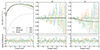 |
Fig. 11. Spectral energy distribution of GX 13+1 in EFE representation as observed by IXPE in bin 1. The left, middle, and right panels show the Stokes parameters I, Q, and U, respectively. The fit is performed in the 2–8 keV energy band using the three IXPE detectors and applying the model tbabs*pollin*(diskbb+bbodyrad). The total model is shown with the solid black line, and diskbb and bbodyrad are shown with the dashed and dotted lines, respectively. The lower subpanels show the residuals between the data and the best fit. The data are rebinned only for plotting purposes. |
Best-fit parameters of the spectropolarimetric model for GX 13+1.
We note that for bins 1 and 5, the spectral and polarimetric properties obtained in the spectropolarimetric analysis agree with the previous results presented in Tables 2 and 4. As we do not have strong detection for the polarimetric properties of bins 2–4, we decided not to present the spectropolarimetric analysis of these bins independently in Table 5, as this does not improve the quality of our results. In bin 1, due to the strong dependency of PD on energy, we applied the pollin model with a constant PA, which gives an improvement by Δχ2 = 9 compared to the fit with the polconst model (which has one parameter less). This improvement corresponds to an F-test probability of ≈3 × 10⁻³.
4. Discussion
4.1. Correlation of the polarimetric behavior with the dip in the light curve
The data analysis presented in Sect. 3 provided us with several significant insights that require interpretation and further reflection. To begin with, we observed significant and anomalous variation in the light curve: the broad dip closer to the end of the observation is not correlated with the regular dips known in the source, as the folding of the MAXI data using the formulae from Iaria et al. (2014) suggests that our observation was made one week before the regular dip. During the dip, we also observed a slight increase in the hardness ratio. It would be natural to expect that polarimetric properties, as hardness and the count rate, have some variations around 6.1–6.3 [MJD–60230]. However, the behavior of the polarimetric properties is not aligned with this variation time-wise. There is a polarimetric anomaly during the dip core state, but the overall trend in PA and PD is not correlated with the dip. PA increases slowly throughout the whole observation, and PD decreases already in bin 2 and then increases in bin 5 without a direct correlation to the dip in the light curve. The inconsistency in the behavior of the spectral and polarimetric properties invites us to search for an explanation for the PA and PD variation outside the regular hardness/intensity changes.
The results of the previous IXPE observations of the X-ray binaries showed that the concept of a rapid and significant change in the PA is not new to this class of objects. The high luminosity of GX 13+1 allowed us to separate the observation into smaller parts and see the slow monotonous rotation of the polarization plane, but the results presented in Fig. 5 are similar to several results that were obtained previously. It is tempting to assume that similar mechanisms might cause the polarimetric behavior of GX 13+1 and that a slow rotation similar to the one presented in Fig. 7 has not been observed previously just due to the lack of statistics or a different approach used in the data analysis. For instance, in Sco X-1, La Monaca et al. (2024) reported that the rotation of the PA with respect to the previous observations (Long et al. 1979) and the jet position angle was around 54°, and the authors explained it with the precession of the jet or with the change in the corona geometry with the transition between the states. However, no sign of an X-ray color variability in GX 13+1 could be associated with these state changes. In the case of Cir X-1 (Rankin et al. 2024), the PA changed by 60° between the two parts of a single observation, but in this case, a clear sign of a corresponding state transition was observed. The difference of 60° between the PA of the hard and soft components of the observation was explained by a switch from the BL to the SL in a tilted NS, as Cir X-1 is a young system (Heinz et al. 2013). GX 13+1, on the other hand, is an older stable system (as is suggested by the companion being a late-evolved K5 III giant) with a high accretion rate; the chances for the rotation axis of the NS to be significantly misaligned relative to the orbital axis are smaller. The results are in many ways also very similar to the polarization that is commonly seen in black hole X-ray binaries (see, e.g., Fig. S6 in Krawczynski et al. 2022 in comparison with Fig. 5). As for Cyg X-1, in GX 13+1 we see the PD during a higher flux rising with energy, while the PD at a (slightly) lower flux is constant. The PA is constant with energy in both cases, but the change in the PA by 60° between the two cases presented in Fig. 5 is significantly different from that in black holes. The rotation of the PA with time was seen recently in the blazar Mrk 421 (Di Gesu et al. 2023). They explained it by the helical magnetic structure in the jet illuminated in the X-rays by a localized shock propagating along this helix. Unfortunately, jets have only been observed in GX 13+1 in the hard state (Allen et al. 2018), and we observed the source in the soft state. It is therefore challenging to imagine that a similar geometry and physics cause the PA rotation in GX 13+1 as in the Mrk 421. In X-ray pulsars, the rotation of the PA with the pulsar phase is routinely observed (Doroshenko et al. 2022, 2023; Tsygankov et al. 2022, 2023), but GX 13+1 is not a pulsar. We conclude that we need to search for a new mechanism that causes the polarimetric behavior of GX 13+1.
4.2. Additional polarimetric component
Figure 7 showed that the source evolves in a straight line (within the uncertainties) in the q − u plane shifted from the origin. Considering this, we tried to decompose the polarized flux into different components with different polarization orientations. It would be problematic to interpret the emission in bins 1 and 5 as coming from two distinct components that differ in PA by 70°, with the rest representing a transitional phase, because a transition like this is unlikely to result in a straight-line trajectory in the q − u plane, particularly given that the flux during bin 4 is lower than during bins 1 and 5. We therefore suggest alternatively that the polarization nature in bins 1 and 5 is predominantly the same, and that the misaligned polarization component is observed in between. A similar model that involves a constant polarized component has previously been proposed to interpret X-ray polarization data from the bright X-ray pulsars LS V +44 17/RX J0440.9+4431 (Doroshenko et al. 2023) and Swift J0243.6+6124 (Poutanen et al. 2024).
We define a constant component corresponding to bin 4 (a period nearly overlapping with the dip, as shown in Fig. 1f). Thus, we subtract absolute Stokes parameters corresponding to bin 4 from the absolute Stokes parameters of each time bin. The resulting normalized Stokes parameters are shown in Fig. 12 with colored points, and the originally observed values are shown with gray points. Their positions are still consistent with a straight line that is now located near the origin. In this scenario, the polarization vectors during bins 1 and 5 are essentially perpendicular to each other (since they lie on the same line in the q − u plane at different sides around the origin), and the radiation observed in bins 2 and 3 appears to be statistically consistent with being unpolarized.
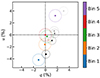 |
Fig. 12. Same as Fig. 7, but the (absolute) Stokes parameters corresponding to bin 4 are subtracted. The gray points are the same as in Fig. 7. |
The picture we see after the subtraction is physically meaningful. A difference of 90° in PAs of bins 1 and 5 could be attributed to changes in the geometry of the scattering or reflecting medium, changes in the scattering optical depth, and the relative brightness changes in the accretion disk, the BL, and the SL. The PA of the permanent component of the polarization (in our assumption, similar to that of bin 4) differs from the PA of the varying component (which we see after the subtraction in Fig. 12) by ≈30°, as clearly visible in the q − u plane. However, as technically, we could have associated the permanent component with any other bin, it is impossible to constrain the angle. The main conclusion here is that this angle is nonzero. To provide this misalignment of the PA between the components associated with the different emission regions within the source, a misalignment in the geometry of the system should be introduced.
4.3. Influence of the variations in the wind
One other possible explanation for the rotation of the polarization plane with time could be the impact of the orbital movement on the polarization arising from the scattering in the accretion bulge. With the high accretion rate known in GX 13+1, some asymmetry in the accretion disk surrounding the NS can be expected. However, GX 13+1 is recognized for having the largest disk in terms of gravitational radius of all observed LMXBs (Tomaru et al. 2020). If a bulge exists, it is therefore probably quite distant from the source. Moreover, we observed a rotation of the polarization plane by ≈70° in the two days of observation. The orbital period of GX 13+1 is 24.5 d. The unknown mechanism that causes the rotation of the polarization plane would need to operate on a shorter timescale.
GX 13+1 is known to have a strong and rapidly changing wind, and evidence for the absorption in the wind comes from the XMM–Newton observation. Scattering in the equatorial wind can produce different polarization patterns in theory, and with this mechanism and with the high inclination of the source, relatively high polarization can be produced easily (see Sunyaev & Titarchuk 1985; Tomaru et al. 2024; Nitindala et al., in prep.). The nature of the polarization variability could be that the observed emission is scattered in the different parts of the wind above the accretion disk. As different absorption features are assumed to come from several distinct parts of the wind with various physical, optical, and geometrical properties, we expect significant differences in the polarimetric behavior. If the line of sight passes close to the edge of the wind, then small variations in the wind opening angle would lead to large variations in the contribution of the scattered component and the polarization degree. We hope to study the correlation between the behavior of the wind and polarimetric properties in the future with simultaneous and IXPE observations.
4.4. Spectral features
All the studies we performed on the spectra of GX 13+1 confirmed the original results from the HID: according to (however limited) IXPE data, there are no significant changes in the spectral behavior with time during the IXPE observation. The study of the radius of the blackbody component Rbb showed no variation in the geometry throughout the observation, with only a slight decrease in the last two bins. In bin 5, the contribution of this component to the total flux also dropped. This adds a challenge to the data interpretation. When we assume that in bin 5, the polarization is produced by the dominating softer disk component, we need to find a way for the disk emission to be polarized at the detected level. The PD coming from the disk is estimated at up to 4% for an inclination of 80° and up to only 1.5% for an inclination of 60° (Loktev et al. 2022) assuming a semi-infinite atmosphere dominated by electron scattering (Chandrasekhar 1960). This means that some scattering in the wind above the disk might need to be introduced. The spectrum contains strong absorption features and GX 13+1 is known to have a strong wind with several absorbing areas. We therefore assume that the wind adds to the polarization of this component. For the harder component, it is more likely to be produced by the BL than the SL. The SL can produce PD up to 1.5% (Bobrikova et al., in prep.), which is not sufficient to explain the high PD we see for higher energies (see Fig. 5). We also expect the polarization from the SL to be orthogonal to the polarization from the disk. We do not see this behavior: all the changes in PA with energy in Fig. 5 and especially in Fig. 3 come from the averaging over time.
We also explored the possibility that the two continua components (diskbb and bbodyrad) each have different polarization properties by fitting the data with the XSPEC model tbabs*(polconst*diskbb+polconst*bbodyrad)*const. We only attempted to apply this model to bin 1 because in this alone, the PD strongly depends on energy, so that it would be easier to resolve the two components. The fit suggested that the diskbb component is almost unpolarized (no significant polarization with the PD < 2.9% is obtained at 99% CL), and the bbodyrad component has a PD of 10% and a PA of −42°. However interesting, this suggestion makes it even harder to understand the relatively high polarization in bin 5, where the disk completely dominates the spectrum. The results of the observation are promising and exciting. They require further study supported by the modeling of the emission from different components and the emission that is scattered in the wind above the disk.
5. Summary
We reported the highly significant detection of polarization from GX 13+1 obtained by IXPE. We performed the polarimetric, spectroscopic, and spectropolarimetric analysis of the IXPE data. The two main components of the spectrum, the soft disk emission and the harder Comptonized component, were described by the diskbb and bbodyrad models, respectively. The spectral analysis was supported by a nonsimultaneous observation performed by XMM–Newton. Due to the high energy resolution of XMM–Newton, we added the gaussian component to describe the broad emission line corresponding to the reflection of the NS surface emission from the disk, four Gaussian absorption lines, gabs, and two edges, edge. For the different parts of the observation, we used the polconst and pollin models for the polarimetric properties. The overall PD of the IXPE data was measured at 1.4% at > 5σ CL, and the PA at −2°.
From the in-depth study of the time variability of the polarimetric properties, we reported the strong rotation of the PA by 70° during the two observation days. The PD varied from 3.2% to the nondetectable and then up to 5.0%. Moreover, we reported the change in the dependence of the PD on energy. At the beginning of the observation, we detected polarization that depended linearly on energy, while in the middle and at the end of the observation, the PD was constant with energy. Some of the previous studies of the WMNSs with IXPE reported a rapid switch of the PA by up to 60°, but the persistent rotation of the polarization plane was presented here for the first time.
We suggested several ways to interpret the results of the data analysis. We studied the correlation of the dip in the light curve with the polarimetric properties and concluded that although the dip corresponds to the anomaly in the PA and PD behavior in the dip-core part of the observation, it is not correlated with the general trends of the polarimetric behavior. We defined a constant polarized component and subtracted it from all the observations. We concluded that the second, time-variable component then is expected to switch the sign of the PD (i.e., the PA rotates by 90°) in the middle of the observation. We also discussed the possible impact of the wind and the unusual state in which we found the source. The observed variations in the PA likely imply a misalignment between the NS spin and the orbital axis. Future polarimetric observations will help us to uncover the nature of this unique phenomenon.
Acknowledgments
The Imaging X-ray Polarimetry Explorer (IXPE) is a joint US and Italian mission. The US contribution is supported by the National Aeronautics and Space Administration (NASA) and led and managed by its Marshall Space Flight Center (MSFC), with industry partner Ball Aerospace (contract NNM15AA18C). The Italian contribution is supported by the Italian Space Agency (Agenzia Spaziale Italiana, ASI) through contract ASI-OHBI-2022-13-I.0, agreements ASI-INAF-2022-19-HH.0 and ASI-INFN-2017.13-H0, and its Space Science Data Center (SSDC) with agreements ASI-INAF-2022-14-HH.0 and ASI-INFN 2021-43-HH.0, and by the Istituto Nazionale di Astrofisica (INAF) and the Istituto Nazionale di Fisica Nucleare (INFN) in Italy. This research used data products provided by the IXPE Team (MSFC, SSDC, INAF, and INFN) and distributed with additional software tools by the High-Energy Astrophysics Science Archive Research Center (HEASARC), at NASA Goddard Space Flight Center (GSFC). We thank the XMM–Newton Project Scientist for approving our DDT request to observe GX 13+1. The research leading to these results has received funding from the European Union’s Horizon 2020 Programme under the AHEAD2020 project (grant agreement 871158). This research has been supported by the Academy of Finland grants 333112, 349144, and 355672 (AB, SVF, JP, VL, AV, APN, SST) and the German Academic Exchange Service (DAAD) travel grant 57525212 (VD). ADM, FLM, SF, FMu, ECo, RF, and PSo are partially supported by MAECI with grant CN24GR08 “GRBAXP: Guangxi-Rome Bilateral Agreement for X-ray Polarimetry in Astrophysics”. This research was also supported by the INAF grant 1.05.23.05.06: “Spin and Geometry in accreting X-ray binaries: The first multifrequency spectro-polarimetric campaign”. IL was supported by the NASA Postdoctoral Program at the Marshall Space Flight Center, administered by Oak Ridge Associated Universities under contract with NASA.
References
- Allen, J. L., Schulz, N. S., Homan, J., et al. 2018, ApJ, 861, 26 [Google Scholar]
- Arnaud, K. A. 1996, ASP Conf. Ser., 101, 17 [Google Scholar]
- Baldini, L., Barbanera, M., Bellazzini, R., et al. 2021, Astropart. Phys., 133, 102628 [NASA ADS] [CrossRef] [Google Scholar]
- Baldini, L., Bucciantini, N., Di Lalla, N., et al. 2022, SoftwareX, 19, 101194 [NASA ADS] [CrossRef] [Google Scholar]
- Bandyopadhyay, R. M., Shahbaz, T., Charles, P. A., & Naylor, T. 1999, MNRAS, 306, 417 [Google Scholar]
- Capitanio, F., Fabiani, S., Gnarini, A., et al. 2023, ApJ, 943, 129 [NASA ADS] [CrossRef] [Google Scholar]
- Chandrasekhar, S. 1960, Radiative Transfer (New York: Dover) [Google Scholar]
- Cocchi, M., Gnarini, A., Fabiani, S., et al. 2023, A&A, 674, L10 [NASA ADS] [CrossRef] [EDP Sciences] [Google Scholar]
- Corbet, R. H. D., Pearlman, A. B., Buxton, M., & Levine, A. M. 2010, ApJ, 719, 979 [Google Scholar]
- D’Aí, A., Iaria, R., Di Salvo, T., et al. 2014, A&A, 564, A62 [CrossRef] [EDP Sciences] [Google Scholar]
- Diaz Trigo, M., Sidoli, L., Parmar, A., & Boirin, L. 2010, AIP Conf. Ser., 1248, 153 [NASA ADS] [Google Scholar]
- Díaz Trigo, M., Sidoli, L., Boirin, L., & Parmar, A. N. 2012, A&A, 543, A50 [NASA ADS] [CrossRef] [EDP Sciences] [Google Scholar]
- Di Gesu, L., Marshall, H. L., Ehlert, S. R., et al. 2023, Nat. Astron., 7, 1245 [NASA ADS] [CrossRef] [Google Scholar]
- Di Marco, A., Costa, E., Muleri, F., et al. 2022, AJ, 163, 170 [NASA ADS] [CrossRef] [Google Scholar]
- Di Marco, A., La Monaca, F., Poutanen, J., et al. 2023a, ApJ, 953, L22 [NASA ADS] [CrossRef] [Google Scholar]
- Di Marco, A., Soffitta, P., Costa, E., et al. 2023b, AJ, 165, 143 [CrossRef] [Google Scholar]
- Doroshenko, V., Poutanen, J., Tsygankov, S. S., et al. 2022, Nat. Astron., 6, 1433 [NASA ADS] [CrossRef] [Google Scholar]
- Doroshenko, V., Poutanen, J., Heyl, J., et al. 2023, A&A, 677, A57 [NASA ADS] [CrossRef] [EDP Sciences] [Google Scholar]
- Fabiani, S., Capitanio, F., Iaria, R., et al. 2024, A&A, 684, A137 [NASA ADS] [CrossRef] [EDP Sciences] [Google Scholar]
- Farinelli, R., Fabiani, S., Poutanen, J., et al. 2023, MNRAS, 519, 3681 [NASA ADS] [CrossRef] [Google Scholar]
- Gilfanov, M., Revnivtsev, M., & Molkov, S. 2003, A&A, 410, 217 [NASA ADS] [CrossRef] [EDP Sciences] [Google Scholar]
- Gnarini, A., Ursini, F., Matt, G., et al. 2022, MNRAS, 514, 2561 [NASA ADS] [CrossRef] [Google Scholar]
- Grindlay, J. E., & Seaquist, E. R. 1986, ApJ, 310, 172 [Google Scholar]
- Heinz, S., Sell, P., Fender, R. P., et al. 2013, ApJ, 779, 171 [Google Scholar]
- Homan, J., van der Klis, M., Wijnands, R., Vaughan, B., & Kuulkers, E. 1998, ApJ, 499, L41 [NASA ADS] [CrossRef] [Google Scholar]
- Iaria, R., Di Salvo, T., Burderi, L., et al. 2014, A&A, 561, A99 [NASA ADS] [CrossRef] [EDP Sciences] [Google Scholar]
- Inogamov, N. A., & Sunyaev, R. A. 1999, Astron. Lett., 25, 269 [NASA ADS] [Google Scholar]
- Kislat, F., Clark, B., Beilicke, M., & Krawczynski, H. 2015, Astropart. Phys., 68, 45 [NASA ADS] [CrossRef] [Google Scholar]
- Krawczynski, H., Muleri, F., Dovčiak, M., et al. 2022, Science, 378, 650 [NASA ADS] [CrossRef] [Google Scholar]
- La Monaca, F., Di Marco, A., Poutanen, J., et al. 2024, ApJ, 960, L11 [NASA ADS] [CrossRef] [Google Scholar]
- Lapidus, I. I., & Sunyaev, R. A. 1985, MNRAS, 217, 291 [NASA ADS] [CrossRef] [Google Scholar]
- Loktev, V., Veledina, A., & Poutanen, J. 2022, A&A, 660, A25 [NASA ADS] [CrossRef] [EDP Sciences] [Google Scholar]
- Long, K. S., Chanan, G. A., Ku, W. H. M., & Novick, R. 1979, ApJ, 232, L107 [NASA ADS] [CrossRef] [Google Scholar]
- Maiolino, T., Laurent, P., Titarchuk, L., Orlandini, M., & Frontera, F. 2019, A&A, 625, A8 [Google Scholar]
- Matsuoka, M., Kawasaki, K., Ueno, S., et al. 2009, PASJ, 61, 999 [Google Scholar]
- Méndez, M., & Belloni, T. M. 2021, Astrophys. Space Sci. Lib., 461, 263 [CrossRef] [Google Scholar]
- NASA High Energy Astrophysics Science Archive Research Center (HEASARC) 2014, Astrophysics Source Code Library [record ascl:1408.004] [Google Scholar]
- Poutanen, J., Tsygankov, S. S., Doroshenko, V., et al. 2024, A&A, submitted [arXiv:2405.08107] [Google Scholar]
- Rankin, J., La Monaca, F., Di Marco, A., et al. 2024, ApJ, 961, L8 [NASA ADS] [CrossRef] [Google Scholar]
- Revnivtsev, M. G., & Gilfanov, M. R. 2006, A&A, 453, 253 [NASA ADS] [CrossRef] [EDP Sciences] [Google Scholar]
- Revnivtsev, M. G., Suleimanov, V. F., & Poutanen, J. 2013, MNRAS, 434, 2355 [NASA ADS] [CrossRef] [Google Scholar]
- Saade, M. L., Kaaret, P., Gnarini, A., et al. 2024, ApJ, 963, 133 [NASA ADS] [CrossRef] [Google Scholar]
- Saavedra, E. A., García, F., Fogantini, F. A., et al. 2023, MNRAS, 522, 3367 [NASA ADS] [CrossRef] [Google Scholar]
- Schnerr, R. S., Reerink, T., van der Klis, M., et al. 2003, A&A, 406, 221 [NASA ADS] [CrossRef] [EDP Sciences] [Google Scholar]
- Shakura, N. I., & Sunyaev, R. A. 1988, Adv. Space Res., 8, 135 [NASA ADS] [CrossRef] [Google Scholar]
- Soffitta, P., Baldini, L., Bellazzini, R., et al. 2021, AJ, 162, 208 [CrossRef] [Google Scholar]
- Sunyaev, R. A., & Titarchuk, L. G. 1985, A&A, 143, 374 [NASA ADS] [Google Scholar]
- Tomaru, R., Done, C., Ohsuga, K., Odaka, H., & Takahashi, T. 2020, MNRAS, 497, 4970 [NASA ADS] [CrossRef] [Google Scholar]
- Tomaru, R., Done, C., & Odaka, H. 2024, MNRAS, 527, 7047 [Google Scholar]
- Tsygankov, S. S., Doroshenko, V., Poutanen, J., et al. 2022, ApJ, 941, L14 [NASA ADS] [CrossRef] [Google Scholar]
- Tsygankov, S. S., Doroshenko, V., Mushtukov, A. A., et al. 2023, A&A, 675, A48 [NASA ADS] [CrossRef] [EDP Sciences] [Google Scholar]
- Ursini, F., Farinelli, R., Gnarini, A., et al. 2023, A&A, 676, A20 [NASA ADS] [CrossRef] [EDP Sciences] [Google Scholar]
- van der Klis, M. 1989, ARA&A, 27, 517 [NASA ADS] [CrossRef] [Google Scholar]
- van der Klis, M. 2000, ARA&A, 38, 717 [NASA ADS] [CrossRef] [Google Scholar]
- Weisskopf, M. C., Soffitta, P., Baldini, L., et al. 2022, JATIS, 8, 026002 [NASA ADS] [Google Scholar]
- White, N. E., & Holt, S. S. 1982, ApJ, 257, 318 [NASA ADS] [CrossRef] [Google Scholar]
- XRISM Science Team 2022, arXiv e-prints [arXiv:2202.05399] [Google Scholar]
All Tables
Results of the pcube analysis performed with various approaches to separate the data.
Best-fit parameters of GX 13+1 spectrum from IXPE data divided into five equal time bins.
All Figures
|
Fig. 1. Normalized Stokes q (a) and u (b) parameters, PA (c), PD (d), hardness ratio (e) with the same colors as in Fig. 2, and the count rate (f) as functions of time as observed by IXPE (all three detectors combined in the energy range 2–8 keV). The light curve is binned in ≈200 s. The dashed vertical blue lines separate the observation into five equal time bins of 10.5 h (Bins 1–5). The region highlighted in yellow corresponds to the dip in the light curve (see Sect. 3.1). Uncertainties are reported at the 68% CL. |
| In the text | |
|
Fig. 2. Hardness-intensity diagram derived from the IXPE data in time bins of 200 s. The colors correspond to the evolution of the data with time, from dark blue at the beginning of the observation to yellow at the end of the observation. |
| In the text | |
|
Fig. 3. Energy-resolved PD and PA averaged over all the IXPE observation, obtained with the pcube algorithm. The data are divided into six 1-keV wide energy bins. Uncertainties are reported at the 68% CL. |
| In the text | |
|
Fig. 4. Polar plot of the PD and PA in the 2–8 keV energy band for the three parts of the observation (pre-dip, dip, and post-dip) and the dip core. Contours are at the 68% CL (dashed lines) and 99% CL (solid lines). |
| In the text | |
|
Fig. 5. Energy dependence of the PD and PA obtained by the pcube algorithm. Left: Pre-dip part of the observation. Right: Post-dip part of the observation. The data are divided into four energy bins: 2–3, 3–4, 4–5.5, and 5.5–8 keV. Uncertainties are reported at 68% CL. |
| In the text | |
|
Fig. 6. Same as Fig. 5, but for the normalized Stokes parameters q and u. Arrows only indicate the label of the energy band. Uncertainties are reported at 68% CL. |
| In the text | |
|
Fig. 7. Time dependence of the normalized Stokes parameters q and u obtained by the pcube algorithm using the data separation into five equal time bins. Uncertainties are reported at the 68% CL. |
| In the text | |
|
Fig. 8. Linear fit of the PA obtained for time bins 1–5 in Fig. 1f. The plot illustrates the rotation of the polarization plane with time. Uncertainties are reported at the 68% CL. |
| In the text | |
|
Fig. 9. Spectral energy distribution of GX 13+1 in EFE representation. The blue crosses show the data from XMM–Newton. The different spectral model components are reported as black lines for diskbb (short dashed), bbodyrad (long dashed), and gaussian (dotted). The total model is shown with a solid black line. The bottom panel shows the residuals between the data and the best fit. The data are rebinned only for plotting purposes. |
| In the text | |
|
Fig. 10. Spectral energy distribution of the source in EFE representation during five equal parts of the observation. Here, only IXPE DU1 is reported as an example, and the data are rebinned for plotting purposes. |
| In the text | |
|
Fig. 11. Spectral energy distribution of GX 13+1 in EFE representation as observed by IXPE in bin 1. The left, middle, and right panels show the Stokes parameters I, Q, and U, respectively. The fit is performed in the 2–8 keV energy band using the three IXPE detectors and applying the model tbabs*pollin*(diskbb+bbodyrad). The total model is shown with the solid black line, and diskbb and bbodyrad are shown with the dashed and dotted lines, respectively. The lower subpanels show the residuals between the data and the best fit. The data are rebinned only for plotting purposes. |
| In the text | |
|
Fig. 12. Same as Fig. 7, but the (absolute) Stokes parameters corresponding to bin 4 are subtracted. The gray points are the same as in Fig. 7. |
| In the text | |
Current usage metrics show cumulative count of Article Views (full-text article views including HTML views, PDF and ePub downloads, according to the available data) and Abstracts Views on Vision4Press platform.
Data correspond to usage on the plateform after 2015. The current usage metrics is available 48-96 hours after online publication and is updated daily on week days.
Initial download of the metrics may take a while.