| Issue |
A&A
Volume 688, August 2024
|
|
|---|---|---|
| Article Number | A95 | |
| Number of page(s) | 9 | |
| Section | Astrophysical processes | |
| DOI | https://doi.org/10.1051/0004-6361/202348758 | |
| Published online | 07 August 2024 | |
Rapid kilonova evolution: Recombination and reverberation effects⋆
1
Cosmic Dawn Center (DAWN), Copenhagen, Denmark
e-mail: This email address is being protected from spambots. You need JavaScript enabled to view it.
2
Niels Bohr Institute, University of Copenhagen, Jagtvej 128, 2200 Copenhagen N, Denmark
3
Astrophysics sub-Department, Department of Physics, University of Oxford, Keble Road, Oxford OX1 3RH, UK
Received:
28
November
2023
Accepted:
5
March
2024
Abstract
Kilonovae (KNe) are one of the fastest types of optical transients known, cooling rapidly in the first few days following their neutron-star merger origin. We show here that KN spectral features go through rapid recombination transitions, with features due to elements in the new ionisation state emerging quickly. Due to time-delay effects of the rapidly expanding KN, a ‘wave’ of these new features passing though the ejecta should be a detectable phenomenon. In particular, isolated line features will emerge as blueshifted absorption features first, gradually evolving into P Cygni features and then pure emission features. In this analysis, we present the evolution of individual exposures of the KN AT2017gfo observed with VLT/X-shooter, which together comprise X-shooter’s first epoch spectrum (1.43 days post-merger). The spectra of these ‘sub-epochs’ show a significant evolution across the roughly one hour of observations, including a decrease in the blackbody temperature and photospheric velocity. The early cooling is even more rapid than that inferred from later photospheric epochs and suggests that a fixed power-law relation between the temperature and time does not describe the data. The cooling constrains the recombination wave, where a Sr II interpretation of the AT2017gfo ∼1 μm feature predicts both a specific timing for the feature emergence and its early spectral shape, including the very weak emission component observed at about 1.43 days. This empirically indicates a strong correspondence between the radiation temperature of the blackbody and the ejecta’s electron temperature. Furthermore, this reverberation analysis suggests that temporal modelling is important for interpreting individual spectra and that higher-cadence spectral series, especially when concentrated at specific times, can provide strong constraints on KN line identifications and the ejecta physics. Given the use of such short-timescale information, we lay out improved observing strategies for future KN monitoring.
Key words: line: profiles / stars: neutron
The work in this paper was based on observations made with European Space Observatory (ESO) telescopes at the Paranal Observatory under programmes 099.D-0382 (principal investigator E. Pian), 099.D-0622 (principal investigator P. D’Avanzo), 099.D-0376 (principal investigator S. J. Smartt). The data are available at http://archive.eso.org. The re-reduced sub-epoch spectra are made available at https://github.com/Sneppen/Kilonova-analysis.
© The Authors 2024
 Open Access article, published by EDP Sciences, under the terms of the Creative Commons Attribution License (https://creativecommons.org/licenses/by/4.0), which permits unrestricted use, distribution, and reproduction in any medium, provided the original work is properly cited.
This article is published in open access under the Subscribe to Open model. This email address is being protected from spambots. You need JavaScript enabled to view it. to support open access publication.
1. Introduction
The temporal data on the kilonova (KN) AT2017gfo have provided several key insights into its evolution and composition. First, the bolometric luminosity follows a power-law-like decay, expected for a large ensemble of rapid neutron-capture process (r-process) isotopes (e.g., Metzger et al. 2010; Wu et al. 2019). Second, follow-up analyses of the spectral energy distribution (SED) have identified P Cygni features proposed to be formed by r-process elements, the first and most obvious being Sr II (Watson et al. 2019), but also potentially La III and Ce III (Domoto et al. 2022), as well as Y II (Sneppen & Watson 2023). These P Cygni profiles change across epochs because they trace the receding photospheric velocity. They also potentially probe differing ionisation states and abundances across the ejecta. This means that more complete radiative transfer modelling of the spectrum can constrain changes in abundances and velocities as a function of time (Gillanders et al. 2022; Vieira et al. 2024, 2023). Lastly, the continuum flux (across early epochs) is remarkably similar to a blackbody in terms of both normalisation and spectral shape (e.g., Sneppen 2023), with the near-infrared (NIR) continuum being especially challenging to reproduce in current numerical simulations of mergers (e.g., Domoto et al. 2022; Collins et al. 2023).
The nightly Very Large Telescope (VLT) spectra taken with the X-shooter spectrograph of the KN AT2017gfo, which is associated with the gravitational wave event GW170817, provide the highest-quality information yet available for studying the rapidly evolving electromagnetic output from the merger of neutron stars (Pian et al. 2017; Smartt et al. 2017). Due to observational constraints, spectra were mostly available with a cadence of around 24 h, limiting the temporal analysis to a time step that is comparable to the time since merger for the early epochs. Temporally important earlier spectra were obtained at telescopes in Chile, Australia, and South Africa (Andreoni et al. 2017; McCully et al. 2017; Shappee et al. 2017; Buckley et al. 2018), though not with the UV-NIR spectral coverage of the X-shooter spectra. While we return to these earlier spectra in a companion paper (Sneppen et al. 2024a), each of these ‘daily’ X-shooter spectra is in fact a composite of several individual exposures taken over approximately an hour. For standard reductions, these exposures are generally analysed together; however, given the brightness of the early KN and the mildly relativistic velocities that smear the spectral line data over tens of thousands of km s−1 and obviate the need for high S/N at high spectral resolution, this is not required. Conversely, given the rapid KN evolution, it is informative to examine these exposures individually. Therefore, in Sect. 2 we re-reduce each exposure of the VLT epoch 1 X-shooter spectrum of AT2017gfo (taken 18–19 August 2017, 1.4 days post-merger). The reduced sub-epoch spectra are made publicly available and are intended as an extension of and addition to the standard reduction presented in Pian et al. (2017) and Smartt et al. (2017). In Sect. 3 we examine the physical information concealed in the differences between these sub-epochs. In Sect. 4.1 we show that, on timescales of the order of several hours, reverberation effects dictate that KN spectral features will emerge rapidly, and as blueshifted absorption components first. Lastly, in Sect. 4.2, given the strong physical constraint from the temporal evolution, we discuss the optimal observing pattern, cadence, and timing for future KNe observations.
2. Sub-epoch reduction and predicted variation
In the following, we outline the data reduction and observational difference between the individual exposures of AT2017gfo made during epoch 1 (1.43 days post-merger). For the first observing night, the medium-resolution, UV (320 nm) to NIR (2480 nm) spectrograph X-shooter took four exposures in nodding mode (Pian et al. 2017), which we label epochs 1.1, 1.2, 1.3, and 1.4. With 10 min exposure times and additional telescope overhead, these exposures monitor the evolution of the transient over about one hour. We focused on this early epoch because it has the highest ratio of exposure timescale to the total time passed since the merger. The four exposures are reduced in nodding mode for the first two and last two exposures (tdiff ≈ 25 min; see Fig. 1, top panel). We also reduced all four exposures individually in stare mode, which shows the same temporal trend as the nodding-mode reduction. However, as the NIR background subtraction is difficult in stare mode, we here focus on the nodding mode constraints.
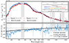 |
Fig. 1. AT2017gfo sub-epoch spectra from X-shooter at 1.43–1.46 days post-merger. Top panel: X-shooter spectra of the first (blue) and second (red) pair of exposures from epoch 1. The timeline of exposures is shown in the top-right inset. Corresponding best-fit models are shown with dashed lines. The spectral shapes are similar, but the later exposures are less luminous and have a lower blackbody temperature. Shaded bars indicate regions with strong tellurics and poorly constrained or noisy regions at the edge of the UVB, VIS, and NIR arms of the spectrograph. Lower panel: flux ratio as a function of wavelength (with the binned weighted mean overlaid), which shows a large fractional change in flux for the UV arm, a gradual evolution across the VIS arm, and a minor and somewhat noisy evolution in the NIR arm. The cooling blackbody prediction is taken from the epoch 1–2 evolution from Sneppen et al. (2023a). The data match the model reasonably well overall. However, the data seem to require a stronger temperature decline at this early time than the model prediction based on the overall epoch 1–2 evolution. |
The spectral reduction pipeline follows those previously detailed in earlier publications (Pian et al. 2017; Smartt et al. 2017), where the X-Shooter pipeline supplied by ESO is used for flat-fielding, order tracing, rectification, and wavelength calibration. The flux calibration of the X-shooter spectra is broadly consistent with contemporaneous photometry from GROND and EFOSC2 (Smartt et al. 2017), DECAM (Cowperthwaite et al. 2017), LDSS (Shappee et al. 2017), Swope (Coulter et al. 2017), and VIRCAM (Tanvir et al. 2017). Therefore, we followed the convention in Pian et al. (2017), Watson et al. (2019), and Sneppen et al. (2023b) and did not artificially scale the spectra to any specific photometric data as they have significant internal scatter. We note that the ‘contemporaneous’ photometric fluxes commonly used for calibration are actually taken over a timescale of two hours, which should be considered a sizeable systematic effect in the reductions, given the rapid nature of the KN evolution at this time.
2.1. Atmospheric observing conditions
On the timescale of the sub-epochs, the atmospheric observing conditions can vary and affect the reduction output in three notable ways.
First, the transmission curves and, by extension, the required telluric corrections, may change. Wavelengths with low atmospheric transmission, such as large parts of the NIR, are most susceptible to these changes, and a minor increase in transmission, for example, could lead to prominent spikes of the telluric-corrected flux. These spikes will be narrow (like the typical width of atmospheric absorption lines) and statistically weak, as the actual observed flux count is small. To determine the impact of this effect, we found both the typical telluric correction estimated from the standard star (taken at comparable airmass immediately following the last exposure) and derived telluric corrections for each sub-epoch individually using Molecfit (Smette et al. 2015; Kausch et al. 2015). Molecfit was run using the standard, well-tested configuration and wavelength ranges (1.12–1.13, 1.47–1.48, 1.80–1.81, and 2.06–2.07 μm) for fitting described in Kausch et al. (2015), though not including the wavelength band around 2.35 μm in the fit due to the weak signal at these wavelengths. These wavelength intervals are standard as they in combination probe the various atmospheric molecules. Because the standard star was only taken at the end of the observing sequence, only Molecfit can constrain the changes in telluric corrections over the individual exposures. Ultimately the difference between the two methods proves minor for the continuum, although fewer artificial and narrow peaks are seen in the intermittent telluric forests redwards of 1300 nm when using Molecfit.
Second, atmospheric dispersion for objects at low inclination is sizeable and chromatic. However, given the atmospheric dispersion correctors on X-shooter and the parallactic angle of the slit, we can verify that the spectral trace shows no skew with wavelength in any of the exposures.
Lastly, the seeing conditions were relatively favourable across the first epoch. The slit width was 1″, 0.9″, and 0.9″ for UVB, VIS, and NIR, and the airmass was in the range 1.42–1.76, which corresponds to a seeing of 0.58″ − 0.74″ (0.59″ − 0.70″) at 500 nm for AT2017gfo (standard star). If the point spread function width becomes comparable to the slit width, slit loss becomes significant and must be accounted for; otherwise, it would lead to an underestimation of the normalisation. Due to the wavelength dependence of seeing, there would also be an increasing slit loss towards shorter wavelengths (which would lead to an underestimation of the temperature). To establish an accurate flux calibration, slit-loss corrections were calculated using the theoretical wavelength dependence on seeing with the average seeing full width at half maximum in each exposure (Fried 1966), identical to the previous reductions (e.g., Pian et al. 2017) and further detailed in Selsing et al. (2019). The slit losses are specifically obtained by integrating this synthetic point spread function over the width of the slits. However, the seeing in epoch 1 is of high enough quality that not accounting for slit-loss corrections provides a similar wavelength-dependent spectral evolution between sub-epochs. Indeed, for all wavelengths λ > 400 nm the resulting spectral ratio (see Fig. 1) is indistinguishable with and without slit-loss corrections, indicating the robustness of the reduction to this systematic effect. In the UV below 400 nm a subtle difference of a few percent is applicable, but this small effect is inconsequential as it is minor and remains below the spectral range of focus in this analysis.
2.2. Predicted kilonova cooling
In a KN atmosphere, the temporal evolution of temperature is set by the competition between adiabatic cooling, radiative cooling and heating from the decay of r-process elements. The decays from an ensemble of isotopes is predicted to provide a heating rate that is well approximated by a single power law (Metzger et al. 2010), which is observationally supported by the AT2017gfo light curve, where the bolometric luminosity from 1 to 6 days post-merger follows a temporal (t) power-law-like decay, Lbol ∝ t−0.95 ± 0.06 (Waxman et al. 2018). The spectra of AT2017gfo in early epochs is observed to be very similar to a blackbody as quantified in Sneppen (2023). In this case, for a spherical photosphere the wavelength-specific luminosity is  , where Rph(t) is the photospheric radius, B(λ, T) is the Planck function with temperature, T, at wavelength λ. The ratio of fluxes at different times for a simple blackbody cooling model is thus merely the ratio of (1) Planck functions of different temperatures and (2) emitting areas. We deliberate on each of these in the following.
The SED ratio is quite sensitive to the evolution in temperature since we sampled the Rayleigh-Jeans tail (i.e., Bλ ≫ hc/(kbT) ∝ T), which has a linear scaling of flux with temperature, the peak (where the flux ratio for blackbodies is proportional to T5), and the exponentially growing discrepancy between the Wien tails. A commonly used prescription for the temperature, T, as a function of the time t since the merger is a power-law relation (e.g., Drout et al. 2017; Waxman et al. 2018):
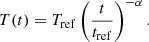 (1)
(1)
Here, α is the cooling power-law index and Tref is the reference temperature at some reference time, tref. Fitting blackbody models to photometry and spectra from 1 to 6 days post-merger suggests the observed temperature has a power-law decline with α = 0.54 ± 0.02 (e.g., Waxman et al. 2018). However, the temperature evolution may be more complex than a single power-law prescription. Indeed, from more advanced spectral modelling that also takes the 1 μm P Cygni and the observed NIR emission lines into account along with a blackbody continuum, it was determined that a single power law does not accurately describe the temperature evolution (Sneppen et al. 2023a). It is initially cooling more rapidly (α ≈ 0.62) at epochs 1–2 (1.4–2.4 days post-merger) and then more slowly (α ≈ 0.4) at epochs 2–3 (2.4–3.4 days post-merger).
The emitting area evolves subtly between the exposures. The atmosphere expands radially with R(t)∝t for homologous expansion. However, as the outer surface becomes increasingly optically thin, the photospheric boundary will recede deeper into the ejecta, so Rph(t)∝tβ with β < 1. Fitting blackbody models from 1–6 days post-merger suggests β = 0.61 ± 0.05 (Waxman et al. 2018). However, the 1 μm P Cygni velocity and the Doppler-corrected blackbody velocity from epochs 1–2 indicate a smaller recession effect with β ≈ 0.75 (Sneppen et al. 2023a). This estimate improves on the previous blackbody velocity by accounting for the relativistic corrections (see Sneppen 2023) and by modelling the observed features in the spectrum (including 1 μm P Cygni and NIR features; see Watson et al. 2019). Changing the emitting area predominantly produces an achromatic shift in the normalisation of the spectrum. Additionally, higher-order chromatic effects (which in this analysis are negligible) may follow from a change in the velocity, such as different light-travel time delays and relativistic corrections (as quantified in Sneppen 2023).
Ultimately, the evolution in epochs 1–2 provides the temporally nearest constraints on the predicted spectral evolution over the first epoch exposures. We therefore define this model as the cooling blackbody prediction, though, a priori, one might expect a slightly faster evolution during epoch 1 itself than the transition from epoch 1–2 would give.
3. Observed sub-epoch evolution
In Fig. 1 we show the epoch 1 spectra from the nodding-mode reduction, which clearly shows that the transient is subtly, but statistically significantly, evolving between the exposures. The drop in flux is particularly pronounced near the blackbody peak and in the UV, while the two spectra converge towards the redder wavelengths of the optical.
To constrain and quantify the spectral evolution, we modelled the spectra as a blackbody perturbed with a P Cygni profile from the three strong lines of Sr II at 1.0037, 1.0327, and 1.0915 μm following the framework detailed in Watson et al. (2019) and Sneppen et al. (2023a,b). The flux drop close to the blue edge of the spectrograph at around 350–400 nm is likely due to Y II and Zr II absorption (Gillanders et al. 2022; Shingles et al. 2023; Sneppen & Watson 2023; Vieira et al. 2023). Hence, the spectral shape in this region of the spectrum is degenerate with the modelling of the UV line opacity. Therefore, we only fitted the wavelengths λ ≥ 400 nm, where the spectrum is better constrained. In the following, we consider the evolution of the continuum and spectral features.
We quickly summarise the parameters investigated. First, the blackbody continuum is described by two parameters, the blackbody temperature, Tobs and velocity/radius, v⊥ = Rph/t, which respectively determine the location of the spectral peak and the normalisation of the spectrum. We note that computing the velocity from the normalisation (ie. angular size) requires an assumption of cosmological distance. Here we assumed for NGC 4993 is 44.2 ± 2.3 Mpc (derived from the cosmic recession velocity of zcosmic = 0.00986 ± 0.00049; Mukherjee et al. 2021; Sneppen et al. 2023b, and assuming Planck cosmology; Planck Collaboration VI 2020), but any typically prescribed distance yields similar results. Second, the 0.7–1.0 μm feature is modelled as a P Cygni profile from the strong three lines of Sr II (4p64d—4p65p) as detailed in Watson et al. (2019). The line profile is parameterised using the spherically symmetric Elementary Supernova model in Jeffery & Branch (1990) with a line optical depth τ, a velocity stratification with a scaling velocity ve, a photospheric velocity of the line v∥, and a maximum ejecta velocity vmax. Further discussion on comparing the inner line-forming region (i.e., v∥) with the emitting area of the blackbody (i.e., v⊥) can be found in Sneppen et al. (2023a).
Notably, this P Cygni framework assumes a pure scattering regime, where any photons absorbed will be re-emitted through the same transition (i.e., without fluorescing into other lines). In the Sr II case, this means that after absorption, the upper energy level, 4p65p, will decay down to the lower level of the transitions, 4p64d, and not the ground state (4p65s). This is a good approximation, as the Sobolev optical depth for the ground-state transition is 1–2 orders of magnitude larger and thus has a much smaller Sobolev escape probability. Conversely, excess emission (relative to the absorption) could potentially be produced from fluorescence from the ground state (i.e., an excitation from 4p65s to 4p65p, which then decays to 4p64d). Such a systematic effect would make it more tenuous to draw tight physical constraints (such as the electron density discussed in Sect. 4.1) from the observed emission/absorption ratio. However, this will likely not strongly affect the temporal formation of the feature and indeed observationally the emission is not boosted but instead largely absent in the 1.4 day spectra.
3.1. Continuum evolution
In the lower panel of Fig. 1 we plot the ratio of fluxes for different wavelength bins. The wavelength-dependent decline in flux predicted from a blackbody cooling in time (indicated with grey shading) traces the UV and optical decline fairly well. We emphasise this is not a fit to the data, but a prediction of a blackbody with a power-law decline of temperature across time derived from comparing epochs 1–2 (see Sect. 2.2). On these short timescales, the evolution in flux from 400 nm to 1000 nm broadly follows the predictions of blackbody cooling. Fitting the blackbody temperature and normalisation for each spectrum independently highlights the evolution in ejecta parameters (see Fig. 2). The best-fit temperature clearly cools between the exposures and the emitting area inferred from the blackbody normalisation suggests that v⊥ has decreased.
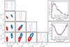 |
Fig. 2. Corner plot indicating the posterior probability distributions of key parameters determined by fitting the spectra in epoch 1.1+1.2 (blue) and epoch 1.3+1.4 (red). The fit parameters are (1) the best-fit observed blackbody temperature, Tobs, (2) the cross-sectional velocity, v⊥, derived from the blackbody normalisation, (3) the photospheric velocity of the 1 μm P Cygni feature, v∥, and (4) the outer ejecta velocity inferred from the 1 μm P Cygni feature, vmax. The dashed grey line in the v⊥ vs. v∥ plot indicates the line of equality, i.e., a spherically symmetric velocity surface. Computing the cross-sectional velocity requires an estimate of the distance to the host; here we assume DL = 44.2 ± 2.3 Mpc, as derived from the Planck cosmology (Planck Collaboration VI 2020), and the cosmological recession velocity of the host galaxy, zcosmic = 0.00986 ± 0.00049 (Mukherjee et al. 2021; Sneppen et al. 2023b). We did not propagate the 5% uncertainty in the absolute luminosity distance into v⊥, as we are interested in the relative change and uncertainties from fitting the spectra themselves. In the right panels, we illustrate the evolution in the continuum (top) and in the 1 μm absorption feature (bottom), which produces the subtle difference in the best-fit parameters. Additional systematic effects such as line-blending could shift the posteriors but are likely to affect sub-epochs in a similar fashion. |
The constraints on the temperature evolution are further quantified in Fig. 3. The inferred α = −0.77 ± 0.06 from the sub-epoch evolution suggests a rapid cooling, which is faster than the 1–2 epoch evolution (α = −0.62 ± 0.01, Sneppen et al. 2023a) and the average 1–6 days post-merger evolution (α = −0.54 ± 0.02, Waxman et al. 2018). This suggests that the early temperature evolution is steeper than inferred from comparing with later epochs. Naturally, the statistical constraining power is lower due to the smaller temporal range, but it is precisely this temporal locality, which makes this estimate complementary in nature to the cross-epoch (but temporally sparse) analysis. That the power-law slope, α, varies with time is a strong indication that a single power-law prescription for the temperature, while a useful and common parameterisation, is an oversimplification.
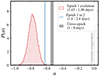 |
Fig. 3. Sub-epoch evolution of the power-law index of cooling, see Eq. (1), of the X-shooter spectra at 1.43 days post-merger (red histogram). The temperature evolution is highly significant (> 10σ from α = 0). The inferred cooling between exposures, α = −0.77 ± 0.06, is more rapid than inferred from the average epoch 1–2 evolution (α = −0.62 ± 0.01, Sneppen et al. 2023a), which is itself more rapid than the cross-epoch analysis over the period 1–6 days post-merger (Waxman et al. 2018). |
That v⊥ decreases may indicate we are observationally probing the recession of the thermalisation surface, which drops deeper into the ejecta as the outer layers become increasingly optically thin. While it is possible that the variable seeing with non-optimal modelling of the slit loss could produce a similar shift, nevertheless, we believe the effect we are observing is real, as there is no other indication of strong slit-loss effects and, as we discuss in Sect. 3.2, the Sr II line also suggests a recession of the photosphere.
3.2. Spectral features
The 1 μm line has a P Cygni nature, which allows constraints to be placed on the velocity of the line-forming region. We show these constraints as part of the model fit in Fig. 2. The line photospheric velocity, v∥, and the outer velocity of the line-forming region, vmax, decrease slightly with time. This independently illustrates and constrains the photospheric surface recession into the ejecta. We note here that, similar to the expanding photosphere method for AT2017gfo presented in Sneppen et al. (2023a), Fig. 2 clearly shows that the thermalisation radius of the blackbody and the photospheric radius of the line decrease coherently and remain consistent with each other across the exposures within the first epoch. The constraints presented in Fig. 2, only include the statistical uncertainty of the fitting model; systematic effects, such as line-blending, time-delay, or reverberation effects for v∥ or the uncertainty in luminosity distance for v⊥, could potentially shift the means of the posteriors, but such effects will likely affect sub-epochs in a similar way, so the temporal evolution of the fitted parameters still follows the trend suggested from the cross-epoch analysis.
As mentioned above, the absorption feature below 400 nm (the UV deficit compared to the blackbody) in the first epochs has been interpreted as tentative evidence of Y II and Zr II lines (Gillanders et al. 2022; Vieira et al. 2023). While we did not fit these ranges in the model, we can still see that the change in flux over these wavelengths is more pronounced between exposures and may indicate increasing opacity at short wavelengths and thus more reprocessing of the light towards redder colours. By later epochs, this absorption feature has disappeared, which may follow from lanthanide (or d-block element) line-blanketing washing out all spectral features below 600–700 nm (Gillanders et al. 2022; Sneppen & Watson 2023).
The NIR spectra are the most difficult to interpret, partly due to the lower S/N, partly because the atmospheric conditions can also change on these timescales (see Sect. 2.1) and partly because some of the strongest emission features appear in the NIR at later epochs, so contributions from such features may also be present and evolving at this time. Such early NIR emission features are still poorly understood, but must be relatively minor at this epoch given the observed continuum. Regardless, the decrease in the bulk flux is least in the NIR and seems to be more or less as predicted from the cooling blackbody framework.
4. Discussion
In this study we have reduced and compared the sub-epochs of the first phase of observations obtained with X-shooter for AT2017gfo. We have highlighted the physical information of the KN these changes on short timescales contain, complementary to the sparse, long timescales between observations. These considerations naturally lead to a discussion on the constraints attainable given observations with a better cadence. In Sect. 4.1 we therefore discuss the additional constraints for line identifications a higher cadence allows, and in Sect. 4.2 we discuss how better to optimise future observing strategies.
4.1. The rapid emergence of spectral lines
Conventionally, line identifications are determined by matching observed features with modelled spectral lines that have consistent transition wavelength and transition probabilities. Thus, identifications follow from analysing the wavelength dimension of the data, while spectra at different times merely serve as different spectral samples for wavelength models. However, for transients with rapid evolution, the timing of the emergence of spectral features is itself a strong prediction for specific line identifications, both in terms of which ionisation states are dominant and in terms of being able to de-blend lines, as we exemplify with two of the proposed identifications below.
Sr II: With a second ionisation energy for Sr of 11.0 eV, typical KN electron densities (i.e., ne ≈ 107 − 109 cm−3), and local thermodynamic equilibrium (LTE) conditions, Sr III (or even higher-ionised species) will become the dominant species for temperatures greater than T ≈ 4300 − 4700 K. For comparison, the emitted blackbody temperature for the ejecta nearest the observer in epoch 1 is T(cos(θ) = 1, tobs = 1.43 days) = 4150 ± 60 K, while the ejecta farther from the observer (which, due to light travel time, is observed at an earlier and hotter time) is T(cos(θ) = β, tobs = 1.43 days) = 4900 ± 70 K (Sneppen 2023). Here, θ is the angle between the direction of expansion and the line of sight. The transition between ionisation states is closely dictated by the temperature because of its exponential dependence in LTE, while the transition time is much less sensitive to the exact electron density. As the ionisation state transitions, the optical depth, τ, of the line will change by orders of magnitude over a few hours. In the radiative transfer equations, this implies a drastic change in the transmission, I = I0e−τ, and thus a rapid formation of the line. This immediately suggests two temporal predictions of the Sr II appearance.
First, spectra taken significantly earlier than about 1.2 day post-merger should not have a 1 μm P Cygni feature due to Sr II (as shown in Fig. 4). This fraction of Sr II was computed assuming LTE with the Saha ionisation equation and the temporal dependence on temperature in Eq. (1) with the cooling rate, α ≈ 0.77, inferred in Sect. 3.1. Applying a lower cooling rate such as that suggested in Waxman et al. (2018) does not significantly change the rapid nature of the recombination1, and the emergence time is only relatively weakly dependent on the exact electron density. In Fig. 5 (right panel) we illustrate how rapidly a Sr II feature would emerge.
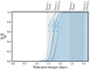 |
Fig. 4. Fraction of Sr in its first ionised state given the time since the merger in LTE. The Sr II is shown as a fraction of total Sr and is transitioning (recombining) from the Sr III state. The blue lines are based on the temperature evolution from the sub-epoch analysis in this paper, while the grey background lines assume the slower cooling in Waxman et al. (2018). Dashed and dotted lines show the fraction assuming different electron densities. Regardless of the exact cooling rate, and across a broad range of electron densities, there is a sharp transition from Sr III to Sr II at 1.4–1.7 days post-merger (or equivalently, for an observer, the absorption will form at 1.0–1.2 days). This suggests that (1) spectra taken just a few hours earlier would have a significantly different Sr II profile and (2) the more distant ejecta will have less Sr II. On the upper axis we show the time of X-shooter epochs 1–2 (Pian et al. 2017; Smartt et al. 2017). We note that, due to light-travel time delays, the more distant ejecta (near the limb) is observed at a different time than the anterior ejecta, as indicated with the grey shaded regions. |
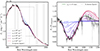 |
Fig. 5. Emergence of a Sr II P Cygni given different electron densities (left) and time post-merger (right). Left: X-shooter epoch 1 spectrum with a model blackbody + Sr II P Cygni feature overlaid. The wavelength-dependent strength of the Sr II feature is modulated by the fractional abundance of singly ionised Sr at the time of observation, tobs = 1.43 days (see Fig. 4). There is only a weak dependence on the electron density as the transition time is a relatively robust prediction in time. This means that the electron density is not tightly constrained, with the majority of the feature indicating a moderate to high electron density of ne ≈ 108 − 109 cm−3. Right: given an electron density ne = 109 cm−3, the corresponding Sr II P Cygni from 0.9 to 1.8 days post-merger in intervals of 0.1 days. The feature rapidly emerges with the reverberation wave, moving from the blueshifted (and nearer) ejecta towards the red. At the time of observation the absorption is fully formed, while the emission is weak due to the decreased fraction of Sr II in the emitting region at the time of emission. This means that the Sr II interpretation can be used to make strong predictions for the timing of the emergence of the feature and the early spectral shape and its evolution. |
Second, the early spectral shape of Sr II is very distinct due to light travel-time effects. The more distant parts of the ejecta (which are earlier and thus hotter) will have more Sr III and less Sr II (Fig. 4). As the distant ejecta is the origin of the emission peak of the P Cygni, and the nearer parts are the origin of the absorption, this would suggest less emission relative to absorption. That is, at early times, a Sr II feature would emerge in absorption blueshifted away from the rest wavelength of the line, but at increasingly later times, as the recombination wave passes through the ejecta, a full P Cygni feature would emerge. This seems to be observationally suggested by the spectra of epoch 1, when the absorption dominates and the emission peak is small (see Fig. 5), as well as at the later epochs, when the emission feature grows in prominence (see Fig. 6). Indeed, the spectra from Gemini-South, taken just an hour after X-shooter, displays a subtle emission peak formed within the narrow time frame, as predicted for a Strontium recombination wave.
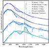 |
Fig. 6. X-shooter epochs 1–3 (from 1.4–3.4 days post-merger) alongside SOAR (Nicholl et al. 2017) and Gemini-South (Chornock et al. 2017) spectra from 1.5 days. As predicted from the 1.4 day blackbody temperature, the recombination wave passing through the ejecta has not reached the equatorial ejecta, resulting in no emission peak. However, just hours later and through the subsequent days, Sr III has recombined into Sr II throughout the ejecta, forming both a blueshifted absorption valley and an emission peak – in essence, a full P Cygni profile. Modelling the continuum as a simple blackbody becomes increasingly tenuous after the first two days – for example, bluewards of the 1 μm feature, around 700 nm the Y II 4d2–4d5p transitions are expected to perturb the SED (Sneppen & Watson 2023), while UV line-blanketing is likely observationally needed to match the spectral shape below λ ⪅ 700 nm (Gillanders et al. 2022). |
In general, given a line ID (i.e., assuming an ionisation energy), the timing of the feature emergence allows the electron density to be determined under LTE conditions. Singly to doubly ionised r-process ejecta with Mejecta = 0.05 M⊙, v = 0.25c (KN characteristic scales from e.g. Kasen et al. 2017), and t = 1.43 days would have a mean electron density of log10(ne/cm−3) = 8.3 − 8.6. Naturally, many systematic effects could shift this estimate substantially, but this density is notably close to that inferred from the 1μm feature given the Sr interpretation, log10(ne/cm−3) ≈ 8 − 9 (see Fig. 5, left panel). Conversely, assuming a broad range of electron densities, one could determine what ionisation energy would be compatible with the line shape and the formation time (i.e., putting strong constraints on the spectral line ID). We emphasise that Sr II (assuming typical KN electron densities) matches the observed feature’s formation is a strong observational indication that the blackbody radiation temperature sets the electron temperature of the ejecta. The optimal constraints on this recombination wave would be a series of spectra detailing the feature shift over several hours (see Fig. 5, right panel).
Earlier spectra than the VLT/X-shooter epoch 1 were taken with Magellan telescopes using the LDSS-3 and MagE spectrographs (at 0.49 and 0.53 days post-merger) and indeed show no 0.7 − 1 μm feature (Shappee et al. 2017). A later spectrum taken using the ANU 2.3 m WiFeS instrument (0.93 days, Andreoni et al. 2017) displays only weak or non-existent absorption, while the South African Large Telescope spectrum (1.18 days, Buckley et al. 2018) has a sizeable absorption component, as predicted from Fig. 5. However, spectral modelling is difficult as these spectra have relatively low S/N and only X-shooter (with its UV-NIR coverage) provides strong constraints on the continuum shape and the 1 μm emission peak. While this emergence time is thus promising for the Sr II interpretation, we leave a detailed comparative analysis for future work (Sneppen et al. 2024a). In a follow-up paper (Sneppen et al. 2024b) we show that a He I interpretation of the 1 μm feature, as introduced and disfavoured in Perego et al. (2022) and argued for in Tarumi et al. (2023), cannot reproduce the observed rapid absorption-to-emission evolution and the time of appearance, both of which seem to be required by the Sr II identification.
At late times, when the Sr II species becomes depopulated, the feature will recede and, again due to reverberation, this will first be in the blueshifted ejecta (i.e., leaving an emission peak that then subsequently fades away). The modelling of the reverberation discussed here mainly focuses on the changing ionisation. The change in the strength of the observed lines and the fading of the spectral continuum with time could produce additional reverberation effects, as discussed in Sneppen et al. (2023b). However, modelling the changing continuum only produces a minor effect at early times because of the softer flux evolution towards the Rayleigh-Jeans tail of the blackbody. Nevertheless, these continuum reverberation effects are essential for understanding the 0.7 − 1 μm feature for intermediate- to late-time evolution when the continuum shifts redwards and the feature’s emission peak is observed to become dominant (see McNeill et al., in prep.).
This reverberation of line formation has primarily focused on ionisation states and not the temporal change of the level populations. We have assumed LTE level populations, and while this means that only 3–7% of the Sr II present will be excited to the 4p64d levels conducive to producing the observed NIR triplet absorption feature (for T in the range 4150 − 4900 K), the high Sr mass fraction for a solar r-process abundance ratio (Lodders et al. 2009; Bisterzo et al. 2014) and the intrinsically very strong transitions means this feature is still expected to be prominent. Using the Boltzmann formula and given the relevant temperatures, 4150–4900 K, one can compute the LTE level population. It has only a weak dependence on temperature relative to the ionisation ratio, for instance when the 4p64d population (the relevant lower level for the transition) changes by a factor of 2 relative to the Sr II ground state, the Sr III/Sr II ratio will change by two orders of magnitude.
Lastly, we emphasise that non-LTE effects and a highly inhomogeneous temperature distribution (and potentially a complex radial and angular density distribution) could make the transitions between ionisation states more gradual. Full radiative transfer modelling of merger simulations is required to explore these dependences. Conversely, strong observational constraints on the emergence of lines can thus potentially reveal insights into the homogeneity of the temperature and the validity of LTE approximations in the ejecta.
Y II: There are two series of lines from the 4d2–4d5p transitions of Y II, one prominent set of lines centred around 760 nm and slightly weaker transitions at 670 nm (Biémont et al. 2011). For the early characteristic expansion velocities (i.e., v ≈ 0.3c), the features from these components will blend together, and the emission and absorption features will produce a series of complex wiggles in the spectra that particularly impact the SED at around 700 nm. However, as velocities decrease, these lines gradually de-blend. When the characteristic velocity recedes below 0.2c (around 4 days post-merger), a P Cygni feature should emerge from the 760 nm lines if yttrium is responsible for these lines. We emphasise that the time when the feature should first appear is a prediction specific to the configuration of atomic levels in Y II. This feature is indeed found to emerge clearly between epochs 3 and 4 for AT2017gfo (Sneppen & Watson 2023).
4.2. Optimal observing strategy
While the timescale of evolution for astrophysical objects, even most transients, is typically much longer than the exposure time, for fast-evolving transients like KNe this is not always the case. The situation is likely to be even more extreme for earlier identifications post-merger than for AT2017gfo. Furthermore, given the emergence of JWST as a viable tool for producing spectra of gamma-ray burst-triggered KNe (Rastinejad et al. 2022; Levan et al. 2024) as well as the improvements to the sensitivity of the Laser Interferometer Gravitational-Wave Observatory and thus the increased distance of most future KNe, reaching a similar signal-to-noise ratio (S/N) as obtained for AT2017gfo will likely require longer exposure times, at least before the advent of the next generation of extremely large ground-based optical telescopes. Thus, in the context of the physical information contained within this short-timescale perspective, it is natural to consider what an optimal observing strategy for future KNe would be.
First, a higher cadence can offer remarkable constraining power for KN modelling – especially at specific temporal intervals (such as around 1.0–1.5 days post-merger), where a sharp transition in ionisation states occurs. As the temperature and density evolution is rapid, species cross the threshold between their ionisation states on a timescale of an hour (i.e., their corresponding spectral lines will emerge or disappear rapidly), the photosphere recedes deeper within the ejecta, and lines de-blend to form interpretable features (see Sect. 4.1). Thus, even if a future KN is only briefly observable (such as for two consecutive hours) due to observational limitations, it is highly constraining to leverage the full temporal span to study the evolutionary trend in parameters.
Second, observing blocks should prioritise several shorter exposures rather than a few long exposures, particularly within the first day or two post-merger. The overhead associated with increased readout time is minor compared to the gain in information from probing the KN evolution between individual exposures. For instance, in the case of AT2017gfo, the four exposures in epoch 1 allow for both temporally resolved nodding and stare-mode reductions. Conversely, with the two longer exposures taken in epoch 2, the temporal information gained is limited, and there is limited possibility of a robustness test of the reduction pipeline across sub-epochs. Ideally, the observing dither pattern would allow a series of individual nodding mode reductions (e.g., in a repeating ABBA dither pattern).
Third, while spectra derived from averaging several exposures for optimal S/N are the standard, early sub-epoch spectra provide additional insights into the time derivative of KN properties and therefore should ideally be reduced and published as well, to provide the full synergy of the time-series spectral evolution.
Or indeed a “combination”, as it may be the first time these freshly formed atoms have ever reached this state.
Acknowledgments
We thank Jonatan Selsing for useful correspondence on the original reduction pipeline in Pian et al. (2017) and Tom Reynolds for the implementation of Molecfit. We thank Stephen Smartt, Stuart Sim, Christine Collins and Luke Shingles for comments and discussions on the evolution of the recombination-wave. The Cosmic Dawn Center (DAWN) is funded by the Danish National Research Foundation under grant DNRF140. AS and DW are funded by the European Union (ERC, HEAVYMETAL, 101071865). Views and opinions expressed are however those of the authors only and do not necessarily reflect those of the European Union or the European Research Council. Neither the European Union nor the granting authority can be held responsible for them.
References
- Andreoni, I., Ackley, K., Cooke, J., et al. 2017, PASA, 34, e069 [NASA ADS] [CrossRef] [Google Scholar]
- Biémont, É., Blagoev, K., Engström, L., et al. 2011, MNRAS, 414, 3350 [Google Scholar]
- Bisterzo, S., Travaglio, C., Gallino, R., Wiescher, M., & Käppeler, F. 2014, ApJ, 787, 10 [NASA ADS] [CrossRef] [Google Scholar]
- Buckley, D. A. H., Andreoni, I., Barway, S., et al. 2018, MNRAS, 474, L71 [NASA ADS] [CrossRef] [Google Scholar]
- Chornock, R., Berger, E., Kasen, D., et al. 2017, ApJ, 848, L19 [NASA ADS] [CrossRef] [Google Scholar]
- Collins, C. E., Bauswein, A., Sim, S. A., et al. 2023, MNRAS, 521, 1858 [NASA ADS] [CrossRef] [Google Scholar]
- Coulter, D. A., Foley, R. J., Kilpatrick, C. D., et al. 2017, Science, 358, 1556 [NASA ADS] [CrossRef] [Google Scholar]
- Cowperthwaite, P. S., Berger, E., Villar, V. A., et al. 2017, ApJ, 848, L17 [CrossRef] [Google Scholar]
- Domoto, N., Tanaka, M., Kato, D., et al. 2022, ApJ, 939, 8 [NASA ADS] [CrossRef] [Google Scholar]
- Drout, M. R., Piro, A. L., Shappee, B. J., et al. 2017, Science, 358, 1570 [NASA ADS] [CrossRef] [Google Scholar]
- Fried, D. L. 1966, J. Opt. Soc. Am., 56, 1380 [NASA ADS] [CrossRef] [Google Scholar]
- Gillanders, J. H., Smartt, S. J., Sim, S. A., Bauswein, A., & Goriely, S. 2022, MNRAS, 515, 631 [NASA ADS] [CrossRef] [Google Scholar]
- Jeffery, D. J., & Branch, D. 1990, in Supernovae, Jerusalem Winter School for Theoretical Physics, eds. J. C. Wheeler, T. Piran, & S. Weinberg, 6, 149 [NASA ADS] [Google Scholar]
- Kasen, D., Metzger, B., Barnes, J., Quataert, E., & Ramirez-Ruiz, E. 2017, Nature, 551, 80 [Google Scholar]
- Kausch, W., Noll, S., Smette, A., et al. 2015, A&A, 576, A78 [NASA ADS] [CrossRef] [EDP Sciences] [Google Scholar]
- Levan, A. J., Gompertz, B. P., Salafia, O. S., et al. 2024, Nature, 626, 737 [NASA ADS] [CrossRef] [Google Scholar]
- Lodders, K., Palme, H., & Gail, H. P. 2009, Landolt Börnstein, 4B, 712 [Google Scholar]
- McCully, C., Hiramatsu, D., Howell, D. A., et al. 2017, ApJ, 848, L32 [NASA ADS] [CrossRef] [Google Scholar]
- Metzger, B. D., Martínez-Pinedo, G., Darbha, S., et al. 2010, MNRAS, 406, 2650 [NASA ADS] [CrossRef] [Google Scholar]
- Mukherjee, S., Lavaux, G., Bouchet, F. R., et al. 2021, A&A, 646, A65 [NASA ADS] [CrossRef] [EDP Sciences] [Google Scholar]
- Nicholl, M., Berger, E., Kasen, D., et al. 2017, ApJ, 848, L18 [NASA ADS] [CrossRef] [Google Scholar]
- Perego, A., Vescovi, D., Fiore, A., et al. 2022, ApJ, 925, 22 [CrossRef] [Google Scholar]
- Pian, E., D’Avanzo, P., Benetti, S., et al. 2017, Nature, 551, 67 [Google Scholar]
- Planck Collaboration VI 2020, A&A, 641, A6 [NASA ADS] [CrossRef] [EDP Sciences] [Google Scholar]
- Rastinejad, J. C., Gompertz, B. P., Levan, A. J., et al. 2022, Nature, 612, 223 [NASA ADS] [CrossRef] [Google Scholar]
- Selsing, J., Malesani, D., Goldoni, P., et al. 2019, A&A, 623, A92 [NASA ADS] [CrossRef] [EDP Sciences] [Google Scholar]
- Shappee, B. J., Simon, J. D., Drout, M. R., et al. 2017, Science, 358, 1574 [NASA ADS] [CrossRef] [Google Scholar]
- Shingles, L. J., Collins, C. E., Vijayan, V., et al. 2023, ApJ, 954, L41 [NASA ADS] [CrossRef] [Google Scholar]
- Smartt, S. J., Chen, T. W., Jerkstrand, A., et al. 2017, Nature, 551, 75 [NASA ADS] [CrossRef] [Google Scholar]
- Smette, A., Sana, H., Noll, S., et al. 2015, A&A, 576, A77 [NASA ADS] [CrossRef] [EDP Sciences] [Google Scholar]
- Sneppen, A. 2023, ApJ, 955, 44 [NASA ADS] [CrossRef] [Google Scholar]
- Sneppen, A., & Watson, D. 2023, A&A, 675, A194 [NASA ADS] [CrossRef] [EDP Sciences] [Google Scholar]
- Sneppen, A., Watson, D., Bauswein, A., et al. 2023a, Nature, 614, 436 [NASA ADS] [CrossRef] [Google Scholar]
- Sneppen, A., Watson, D., Poznanski, D., et al. 2023b, A&A, 678, A14 [NASA ADS] [CrossRef] [EDP Sciences] [Google Scholar]
- Sneppen, A., Watson, D., Damgaard, R., et al. 2024a, A&A, in press https://doi.org/10.1051/0004-6361/202450317 [NASA ADS] [CrossRef] [EDP Sciences] [Google Scholar]
- Sneppen, A., Watson, D., Damgaard, R., et al. 2024b, A&A, submitted [arXiv:2407.12907] [Google Scholar]
- Tanvir, N. R., Levan, A. J., González-Fernández, C., et al. 2017, ApJ, 848, L27 [CrossRef] [Google Scholar]
- Tarumi, Y., Hotokezaka, K., Domoto, N., & Tanaka, M. 2023, ArXiv e-prints [arXiv:2302.13061] [Google Scholar]
- Vieira, N., Ruan, J. J., Haggard, D., et al. 2023, ApJ, 944, 123 [NASA ADS] [CrossRef] [Google Scholar]
- Vieira, N., Ruan, J. J., Haggard, D., et al. 2024, ApJ, 962, 33 [NASA ADS] [CrossRef] [Google Scholar]
- Watson, D., Hansen, C. J., Selsing, J., et al. 2019, Nature, 574, 497 [NASA ADS] [CrossRef] [Google Scholar]
- Waxman, E., Ofek, E. O., Kushnir, D., & Gal-Yam, A. 2018, MNRAS, 481, 3423 [NASA ADS] [CrossRef] [Google Scholar]
- Wu, M.-R., Barnes, J., Martínez-Pinedo, G., & Metzger, B. D. 2019, Phys. Rev. Lett., 122, 062701 [NASA ADS] [CrossRef] [Google Scholar]
All Figures
|
Fig. 1. AT2017gfo sub-epoch spectra from X-shooter at 1.43–1.46 days post-merger. Top panel: X-shooter spectra of the first (blue) and second (red) pair of exposures from epoch 1. The timeline of exposures is shown in the top-right inset. Corresponding best-fit models are shown with dashed lines. The spectral shapes are similar, but the later exposures are less luminous and have a lower blackbody temperature. Shaded bars indicate regions with strong tellurics and poorly constrained or noisy regions at the edge of the UVB, VIS, and NIR arms of the spectrograph. Lower panel: flux ratio as a function of wavelength (with the binned weighted mean overlaid), which shows a large fractional change in flux for the UV arm, a gradual evolution across the VIS arm, and a minor and somewhat noisy evolution in the NIR arm. The cooling blackbody prediction is taken from the epoch 1–2 evolution from Sneppen et al. (2023a). The data match the model reasonably well overall. However, the data seem to require a stronger temperature decline at this early time than the model prediction based on the overall epoch 1–2 evolution. |
| In the text | |
|
Fig. 2. Corner plot indicating the posterior probability distributions of key parameters determined by fitting the spectra in epoch 1.1+1.2 (blue) and epoch 1.3+1.4 (red). The fit parameters are (1) the best-fit observed blackbody temperature, Tobs, (2) the cross-sectional velocity, v⊥, derived from the blackbody normalisation, (3) the photospheric velocity of the 1 μm P Cygni feature, v∥, and (4) the outer ejecta velocity inferred from the 1 μm P Cygni feature, vmax. The dashed grey line in the v⊥ vs. v∥ plot indicates the line of equality, i.e., a spherically symmetric velocity surface. Computing the cross-sectional velocity requires an estimate of the distance to the host; here we assume DL = 44.2 ± 2.3 Mpc, as derived from the Planck cosmology (Planck Collaboration VI 2020), and the cosmological recession velocity of the host galaxy, zcosmic = 0.00986 ± 0.00049 (Mukherjee et al. 2021; Sneppen et al. 2023b). We did not propagate the 5% uncertainty in the absolute luminosity distance into v⊥, as we are interested in the relative change and uncertainties from fitting the spectra themselves. In the right panels, we illustrate the evolution in the continuum (top) and in the 1 μm absorption feature (bottom), which produces the subtle difference in the best-fit parameters. Additional systematic effects such as line-blending could shift the posteriors but are likely to affect sub-epochs in a similar fashion. |
| In the text | |
|
Fig. 3. Sub-epoch evolution of the power-law index of cooling, see Eq. (1), of the X-shooter spectra at 1.43 days post-merger (red histogram). The temperature evolution is highly significant (> 10σ from α = 0). The inferred cooling between exposures, α = −0.77 ± 0.06, is more rapid than inferred from the average epoch 1–2 evolution (α = −0.62 ± 0.01, Sneppen et al. 2023a), which is itself more rapid than the cross-epoch analysis over the period 1–6 days post-merger (Waxman et al. 2018). |
| In the text | |
|
Fig. 4. Fraction of Sr in its first ionised state given the time since the merger in LTE. The Sr II is shown as a fraction of total Sr and is transitioning (recombining) from the Sr III state. The blue lines are based on the temperature evolution from the sub-epoch analysis in this paper, while the grey background lines assume the slower cooling in Waxman et al. (2018). Dashed and dotted lines show the fraction assuming different electron densities. Regardless of the exact cooling rate, and across a broad range of electron densities, there is a sharp transition from Sr III to Sr II at 1.4–1.7 days post-merger (or equivalently, for an observer, the absorption will form at 1.0–1.2 days). This suggests that (1) spectra taken just a few hours earlier would have a significantly different Sr II profile and (2) the more distant ejecta will have less Sr II. On the upper axis we show the time of X-shooter epochs 1–2 (Pian et al. 2017; Smartt et al. 2017). We note that, due to light-travel time delays, the more distant ejecta (near the limb) is observed at a different time than the anterior ejecta, as indicated with the grey shaded regions. |
| In the text | |
|
Fig. 5. Emergence of a Sr II P Cygni given different electron densities (left) and time post-merger (right). Left: X-shooter epoch 1 spectrum with a model blackbody + Sr II P Cygni feature overlaid. The wavelength-dependent strength of the Sr II feature is modulated by the fractional abundance of singly ionised Sr at the time of observation, tobs = 1.43 days (see Fig. 4). There is only a weak dependence on the electron density as the transition time is a relatively robust prediction in time. This means that the electron density is not tightly constrained, with the majority of the feature indicating a moderate to high electron density of ne ≈ 108 − 109 cm−3. Right: given an electron density ne = 109 cm−3, the corresponding Sr II P Cygni from 0.9 to 1.8 days post-merger in intervals of 0.1 days. The feature rapidly emerges with the reverberation wave, moving from the blueshifted (and nearer) ejecta towards the red. At the time of observation the absorption is fully formed, while the emission is weak due to the decreased fraction of Sr II in the emitting region at the time of emission. This means that the Sr II interpretation can be used to make strong predictions for the timing of the emergence of the feature and the early spectral shape and its evolution. |
| In the text | |
|
Fig. 6. X-shooter epochs 1–3 (from 1.4–3.4 days post-merger) alongside SOAR (Nicholl et al. 2017) and Gemini-South (Chornock et al. 2017) spectra from 1.5 days. As predicted from the 1.4 day blackbody temperature, the recombination wave passing through the ejecta has not reached the equatorial ejecta, resulting in no emission peak. However, just hours later and through the subsequent days, Sr III has recombined into Sr II throughout the ejecta, forming both a blueshifted absorption valley and an emission peak – in essence, a full P Cygni profile. Modelling the continuum as a simple blackbody becomes increasingly tenuous after the first two days – for example, bluewards of the 1 μm feature, around 700 nm the Y II 4d2–4d5p transitions are expected to perturb the SED (Sneppen & Watson 2023), while UV line-blanketing is likely observationally needed to match the spectral shape below λ ⪅ 700 nm (Gillanders et al. 2022). |
| In the text | |
Current usage metrics show cumulative count of Article Views (full-text article views including HTML views, PDF and ePub downloads, according to the available data) and Abstracts Views on Vision4Press platform.
Data correspond to usage on the plateform after 2015. The current usage metrics is available 48-96 hours after online publication and is updated daily on week days.
Initial download of the metrics may take a while.