| Issue |
A&A
Volume 678, October 2023
|
|
|---|---|---|
| Article Number | A14 | |
| Number of page(s) | 13 | |
| Section | Cosmology (including clusters of galaxies) | |
| DOI | https://doi.org/10.1051/0004-6361/202346306 | |
| Published online | 02 October 2023 | |
Measuring the Hubble constant with kilonovae using the expanding photosphere method
1
Cosmic Dawn Center (DAWN), Denmark
e-mail: This email address is being protected from spambots. You need JavaScript enabled to view it.
2
Niels Bohr Institute, University of Copenhagen, Blegdamsvej 17, 2100 Copenhagen, Denmark
3
School of Physics and Astronomy, Tel Aviv University, Tel Aviv 69978, Israel
4
Cahill Center for Astrophysics, California Institute of Technology, 1200 E. California Boulevard, Pasadena, CA 91125, USA
5
GSI Helmholtzzentrum für Schwerionenforschung, Planckstraße 1, 64291 Darmstadt, Germany
6
Astrophysical Big Bang Laboratory, RIKEN Cluster for Pioneering Research, 2-1 Hirosawa, Wako, Saitama 351-0198, Japan
7
Helmholtz Forschungsakademie Hessen für FAIR, GSI Helmholtzzentrum für Schwerionenforschung, Planckstraße 1, 64291 Darmstadt, Germany
8
DARK, Niels Bohr Institute, University of Copenhagen, Jagtvej 128, 2200 Copenhagen, Denmark
Received:
2
March
2023
Accepted:
19
July
2023
Abstract
While gravitational wave (GW) standard sirens from neutron star (NS) mergers have been proposed to offer good measurements of the Hubble constant, we show in this paper how a variation of the expanding photosphere method (EPM) or spectral-fitting expanding atmosphere method, applied to the kilonovae (KNe) associated with the mergers, can provide an independent distance measurement to individual mergers that is potentially accurate to within a few percent. There are four reasons why the KN-EPM overcomes the major uncertainties commonly associated with this method in supernovae: (1) the early continuum is very well-reproduced by a blackbody spectrum, (2) the dilution effect from electron scattering opacity is likely negligible, (3) the explosion times are exactly known due to the GW detection, and (4) the ejecta geometry is, at least in some cases, highly spherical and can be constrained from line-shape analysis. We provide an analysis of the early VLT/X-shooter spectra AT2017gfo showing how the luminosity distance can be determined, and find a luminosity distance of DL = 44.5 ± 0.8 Mpc in agreement with, but more precise than, previous methods. We investigate the dominant systematic uncertainties, but our simple framework, which assumes a blackbody photosphere, does not account for the full time-dependent three-dimensional radiative transfer effects, so this distance should be treated as preliminary. The luminosity distance corresponds to an estimated Hubble constant of H0 = 67.0 ± 3.6 km s−1 Mpc−1, where the dominant uncertainty is due to the modelling of the host peculiar velocity. We also estimate the expected constraints on H0 from future KN-EPM-analysis with the upcoming O4 and O5 runs of the LIGO collaboration GW-detectors, where five to ten similar KNe would yield 1% precision cosmological constraints.
Key words: distance scale / cosmological parameters / stars: neutron / radiation mechanisms: thermal
© The Authors 2023
 Open Access article, published by EDP Sciences, under the terms of the Creative Commons Attribution License (https://creativecommons.org/licenses/by/4.0), which permits unrestricted use, distribution, and reproduction in any medium, provided the original work is properly cited.
This article is published in open access under the Subscribe to Open model. This email address is being protected from spambots. You need JavaScript enabled to view it. to support open access publication.
1. Introduction
A precise measurement of the Hubble constant, H0, is critical to the study of cosmology. With the growing precision of cosmological studies has followed an increasing tension, currently significant at 5σ, between measurements of the H0 from type Ia supernovae (SNe) calibrated with Cepheids observed by the SH0ES collaboration (for Supernova H0 for the Equation of State Riess et al. 2022) and Planck observations of the cosmic microwave background radiation assuming a flat ΛCDM cosmological model (Planck Collaboration VI 2020). If these measurements are correct, this would suggest the standard cosmological paradigm, Lambda-cold dark matter (ΛCDM), cannot simultaneously fit observations at all redshifts, necessitating modifications to the cosmological model or to the physics of the early Universe, perhaps in the form of early dark energy (e.g., Poulin et al. 2019; Kamionkowski & Riess 2022).
The ΛCDM paradigm may still be valid if unaccounted-for systematic effects have biased the inferred H0 from either framework. For the local H0 constraints this includes, but is not limited to, issues in modelling extinction in type Ia SNe Wojtak & Hjorth (2022) or Cepheids (Mörtsell et al. 2022), Cepheid metallicity correction (Efstathiou 2020), host-galaxy properties (Steinhardt et al. 2020), and different populations of SNe Ia at low-z and high-z (Jones et al. 2018; Rigault et al. 2020). Given the many potential systematics, high-quality independent measurements of the Hubble constant on local cosmic distance scales can provide crucial evidence in the interpretation of the H0 divergence.
Many independent probes have been developed, including time-delays of gravitationally lensed, variable sources (Birrer et al. 2020; Wong et al. 2020), megamaser distance measurements (Pesce et al. 2020), active galactic nucleus (AGN) dust reverberation (Hönig et al. 2014; Yoshii et al. 2014), γ-ray attenuation by extragalactic background light Domínguez et al. (2019), and the gravitational wave (GW) standard siren (Schutz 1986; Abbott et al. 2017). However, any conclusive interpretation remains elusive due to limited statistics and/or modelling uncertainties for all these methods. It has been argued that a rapid growth in GW sensitivity and an abundance of optical counterparts with redshifts could enable 1σ constraints at the 2% level using neutron star (NS) merger standard sirens within a few years (Chen et al. 2018). The tightest current H0 constraint comes from combining very-long-baseline interferometry constraints with the GW standard siren, yielding fractional uncertainty of 7% (Hotokezaka et al. 2019). It has also been argued that using the optical transient kilonova (KN) associated with NS merger events it might be possible to provide estimates of H0 (Doctor 2020; Coughlin et al. 2020), though constraints are comparatively poor and model-dependent compared to the standard siren.
A P Cygni feature associated with a transition of Sr II was identified in the spectra of AT2017gfo, the kilonova associated with GW170817 (Watson et al. 2019). An additional P Cygni feature from transitions in Y II was subsequently identified in later epochs (Sneppen & Watson 2023). These P Cygni features have provided the first positive identification of freshly formed r-process elements, and allows the velocity and geometry of the kilonova to be probed. A recent analysis (Sneppen et al. 2023) shows that the outer ejecta in AT2017gfo is spherically symmetric, which is not a generic outcome in existing theoretical models of merger ejecta (e.g., Kasen et al. 2015; Martin et al. 2015; Collins et al. 2023; Just et al. 2023). Future studies will need to explore in detail the exact conditions under which the ejecta becomes highly spherical. However, this sphericity, in conjunction with the clear blackbody continuum of early spectra does make AT2017gfo and similar kilonovae potentially excellent high-precision cosmological probes.
We show in Sect. 3.1 how a variant of the expanding photosphere method (EPM, Kirshner & Kwan 1974) applied to KNe provides a novel and self-consistent estimator of cosmological distances with 2% percent fractional uncertainty to AT2017gfo. In Sect. 3.2, we present the corresponding H0 constraints, which, as they are dominated by peculiar velocity uncertainties, remain broadly consistent with both late and early Universe measurements. We discuss systematic effects in Sect. 4. However, it is not our intent in this paper to make a definitive estimate of H0 because we do not fully account for all spectral effects or for the major time-delay effects, which require more sophisticated and self-consistent 2D or 3D radiative transfer modelling. Rather, we intend to show that a very accurate measurement of H0 may be made using the kilonova AT2017gfo, and we show in Sect. 5 how the highly constrained distance suggests that a handful of future kilonova detections may provide sub-percent precision constraints on H0 entirely independent of the cosmic distance ladder.
2. Methodology
The series of spectra of AT2017gfo taken with the medium-resolution ultraviolet (UV) to near-infrared (NIR) spectrograph, X-shooter, mounted at the Very Large Telescope at the European Southern Observatory, provides the most detailed information of any kilonova to date. Spectra were taken daily from 1.43 days after the event for 19 days, and show a temporal evolution of continuum, emission, and absorption features (Smartt et al. 2017; Pian et al. 2017). The spectra we use here are the same as those used in Sneppen et al. (2023) and follow the data reduction presented there and in Pian et al. (2017). In the following section we deliberate on the spectral properties of both the blackbody continuum and the P Cygni profiles of Sr II, and then review the methodology and assumptions associated with the expanding photosphere method in Sect. 2.3.
2.1. Blackbody continuum of AT2017gfo
Previous studies have established that the spectra from the earliest epochs of AT2017gfo are well-approximated by a blackbody spectrum (Malesani et al. 2017; Waxman et al. 2018; Villar et al. 2017; Cowperthwaite et al. 2017; Nicholl et al. 2017; Arcavi 2018; Drout et al. 2017; Shappee et al. 2017; Watson et al. 2019). For a blackbody, the specific luminosity of the photosphere is set by the emitting area (which for a spherical expansion is set by the radius of the photosphere,  ), the Planck function B(λ, Teff) at a temperature Teff, and the relativistic Doppler and time-delay correction (f(β)) for a photosphere expanding with a velocity β = vph/c:
 (1)
(1)
Notably, for SNe the photospheric radius is above the thermalisation radius, due to the large contribution of electron-scattering opacity to the total opacity (Eastman et al. 1996; Dessart & Hillier 2005; Dessart et al. 2015). However, in KN ejecta the electron scattering opacity is small compared to the opacity of bound–bound transitions. This ratio is lower for two reasons. First, the opacity of bound–bound transitions is higher by several orders of magnitude due to the multiplicity of lines of r-process elements and the complexity of valence electron structure of elements within the r-process composition (Kasen et al. 2013), though this is somewhat lower for the lighter r-process elements. Secondly, the KN ejecta is composed of typically neutral singly- or doubly-ionised heavy elements, so the number of free electrons per unit mass is O(102) smaller than the typical value for ionised hydrogen. Thus, for the analysis of kilonovae we can assume the photospheric radius derived from the line is indeed at the thermalisation depth of the blackbody and no significant correction or ‘dilution factor’ for electron opacity is required to determine the luminosity or distance.
2.2. P Cygni modelling
The largest deviation from a blackbody detected in the early spectra is around 810 nm (Smartt et al. 2017), and is interpreted as the strong resonance lines at 1.0037, 1.0327, and 1.0915 μm from Sr+ in the ejecta (Watson et al. 2019). These lines are modelled using the P Cygni profile prescription described below, with the relative strengths of each of the lines set by the local thermodynamic equilibrium relation. A less prominent P Cygni feature at 0.76 μm likely associated with transition lines of Y+ has also been observed in the kilonova (Sneppen & Watson 2023).
The P Cygni profile is characteristic of expanding envelopes where the same spectral line yields both an emission peak near the rest wavelength and a blueshifted absorption feature (Jeffery & Branch 1990). The peak is formed by true emission or by scattering into the line of sight, while the trough is due to absorption or scattering of photospheric photons out of the line of sight. As the latter is in the front of the ejecta this component is blueshifted. The P Cygni profile is characterised by several properties of the KN atmosphere. The optical depth determines the strength of absorption and emission, while the velocity of the ejecta sets the wavelength of the absorption minimum. For this analysis we use the implementation1 of the P Cygni profile in the Elementary Supernova model (Jeffery & Branch 1990), where the profile is expressed in terms of the rest wavelength λ0, the line optical depth τ, with velocity stratification parametrised with a scaling velocity ve, a photospheric velocity vph, and a maximum ejecta velocity vmax. Furthermore, we include a parameter describing the enhancement or suppression of the P Cygni emission to improve the fit to the line shape. This parameter does not impact our constraints as it is predominantly the absorption component that provides the velocity constraints. While this parametrisation assumes an optical depth with an exponential decay in velocity (i.e., τ(v) = τ0 ⋅ e−v/ve; Thomas et al. 2011), we note that we can equivalently assume a power-law decay with the resulting constraints being indistinguishable. This P Cygni fitting framework follows the convention already established in Watson et al. (2019) and Sneppen et al. (2023) for fitting AT2017gfo.
To account for ejecta asphericity, we include in our P Cygni profile prescription an additional and free-to-vary eccentricity e and viewing angle θinc. This allows an independent probe of the sphericity by fitting the line shape to an expanding ellipsoidal photosphere. While in general constraints from the shape of spectral lines on the asymmetry of ejecta is degenerate with the viewing angle (Hoeflich et al. 1996), in this case the radio jet, the precision astrometry, and the gravitational standard siren in conjunction provide strong priors on the inclination angle of the merger, with θinc = 22° ± 3° (Mooley et al. 2018, 2022). With a strong prior on the inclination angle, we can fit the line shape to constrain the asphericity of the ellipse, v⊥/v∥. We find 1.01 ± 0.01 and 0.995 ± 0.006 for epochs 1 and 2, respectively (Sneppen et al. 2023). We note that this uncertainty is only the statistical uncertainty of fitting the model to the data. Systematic effects such as blending with other possible (as yet unidentified) lines or time-delay and/or reverberation effects may shift these constraints. However, we argue that these systematic effects must be relatively small given the consistency in distance across statistically independent epochs as elaborated in Sect. 4.8.
2.3. The expanding photosphere method
The expanding photosphere method (EPM) is a tool to measure the luminosity distance DL to objects with large amounts of ejected material (Baade 1926; Wesselink 1946; Kirshner & Kwan 1974). While the methodology was first developed for core-collapse SNe, Sneppen et al. (2023) demonstrated its applicability to KNe. The EPM assumes a simplified model of the ejecta as a photosphere in homologous and spherically symmetric expansion, so the photosphere size follows directly from the expansion velocity, measured from a Doppler line shift, and the time since explosion: Rph = vph(t − te). In KNe homologous expansion is expected to set in rapidly: less than a second after the merger for dynamical ejecta (Rosswog et al. 2014) and up to 101 − 102 s for the post-merger ejecta (Kasen et al. 2015). There is now also good evidence that the outer ejecta of AT2017gfo was spherical (Sneppen et al. 2023). However, the sphericity assumption can be relaxed if the symmetry of the explosion can be quantified. Modelling and propagating these symmetry constraints yields a cross-sectional radius of the form
![Mathematical equation: $$ \begin{aligned} R_{\rm \perp } = v_{\rm \perp } (t-t_{\rm e}) = v_{\rm ph} (t-t_{\rm e}) \left[\frac{v_{\rm \perp }}{v_{\rm ph}}\right] ,\end{aligned} $$](/articles/aa/full_html/2023/10/aa46306-23/aa46306-23-eq3.gif) (2)
(2)
where the ratio in the square bracket and vph come directly from the line Doppler shift and line shape constraints.
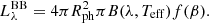
The luminosity distance can be estimated by comparing the luminosity of the blackbody to the observed dereddened flux. The specific total luminosity inferred from observations is 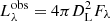 , where Fλ is the wavelength specific flux, while the overall luminosity of a blackbody from Eq. (1) is
 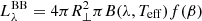 . Combining these with Eq. (2), the luminosity distance is thus
![Mathematical equation: $$ \begin{aligned} D_{\rm L} = v_{\rm ph} (t-t_{\rm e}) \left[\frac{v_{\rm \perp }}{v_{\rm ph}}\right] \sqrt{\frac{\pi B(\lambda ,T_{\rm eff}) f(\beta )}{F_\lambda } } .\end{aligned} $$](/articles/aa/full_html/2023/10/aa46306-23/aa46306-23-eq6.gif) (3)
(3)
Crucially, this estimate requires no calibration with known distances and is entirely independent of the cosmic distance ladder. Furthermore, for KNe the precise explosion time (te) is provided by the gravitational wave signal. This ensures that each spectrum can yield an estimate of distance that is statistically independent from every other epoch, thereby testing the internal consistency and robustness of this EPM framework. As mentioned above, the blackbody colour and luminosity temperatures are likely to be very close (i.e., the dilution-factor correction is negligible), and the factor f(β) can in principle be calculated analytically. There are therefore no major unknown quantities in the equation and each measured quantity (flux, velocity, time, and temperature) is well constrained.
Comparing the EPM estimated distance to the KN with the cosmological redshift of the host galaxy, we can now determine an independent constraint on the Hubble constant. To good approximation for z ≪ 1, Hubble’s law gives the luminosity distance (with q0 = −0.53 for the Planck cosmological model; Planck Collaboration VI 2020):
 (4)
(4)
Here zcosmic is the recession velocity corresponding to pure Hubble flow (i.e., correcting for the peculiar velocity due to large-scale structure, zcosmic = zCMB − zpec).
3. Application to AT2017gfo
3.1. Estimating the luminosity distance
We fit the spectra with a Planck function and a P Cygni line profile associated with the Sr+ triplet at 1.0037, 1.0327, and 1.0915 μm, to measure both the blackbody flux and the velocity of expansion. The X-shooter spectrum and the best-fit models for each of the first two epochs are illustrated in Fig. 1. Despite the simplicity of the methodology, the analysis provides a good fit to the data, consistent over multiple epochs. Using the EPM framework we deduce the luminosity distances for each epoch independently, with the posterior probability distributions shown in Fig. 2. This illustrates a few things of note. First, in each epoch the posterior distribution remains uni-modal with a single maximum in the likelihood landscape. Second, the statistical uncertainty in each epoch is small, at the level of 2–3%. However, the difference between the distance measure for each epoch, which are statistically independent, is larger than this, at the level of about 5% (i.e., comparable to the peculiar velocity uncertainty). This corresponds to a 1.9σ discrepancy, which may indicate that the uncertainty on the distances is somewhat underestimated. The most obvious potential culprits in underestimating the uncertainty are the tight sphericity constraints from the line shape fitting and the dust extinction due to the host galaxy. We discuss the sphericity constraints in Sect. 4.8, and the dust correction in Sect. 4.4.
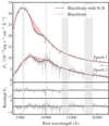 |
Fig. 1. Spectrum and fit of the kilonova AT2017gfo spectrum for epochs 1 and 2 (days +1.43 and +2.42). The dotted line on the right side indicates the offset (7 × 10⁻¹⁷ erg cm−2 s−1 Å−1) added to the first epoch spectrum, the dark shaded bars indicate telluric regions, and the light shaded bars indicate overlapping noisy regions at the edges of the UVB, VIS, and NIR arms. |
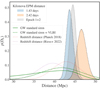 |
Fig. 2. Posterior probability distributions of luminosity distances for each epoch sampled with MCMC runs. The distance estimate from the standard siren with and without very long baseline interferometry radio inclination angle data (Mooley et al. 2018; Hotokezaka et al. 2019) are shown as dashed and solid green lines, respectively. Cosmological redshift distances are also plotted for H0 = 67.36 ± 0.54 (Planck Collaboration VI 2020) (dotted red) and H0 = 73.03 ± 1.04 (Riess et al. 2022) (dotted purple). |
The estimated luminosity distance for the first and second epochs yield respectively 43.7 ± 0.9 Mpc and 46.6 ± 1.2 Mpc, which yields a joint constraint from epoch 1+2 of 44.5 ± 0.8 Mpc. The unweighted average of these measurements yields 45.2 ± 1.5 Mpc, which would suggest the fractional distance uncertainty is of the order of a few percent. These EPM distances are consistent with earlier distance estimates to the host galaxy NGC 4993, including from surface brightness fluctuations (Cantiello et al. 2018), the fundamental plane (Hjorth et al. 2017), GW standard siren measurements (Abbott et al. 2017), and combining the GW standard siren with constraints on inclination angle from very-long-baseline interferometry (Hotokezaka et al. 2019).
3.2. Constraints on H0
The recession velocity of the host-galaxy group is well constrained: zCMB = 0.01110 ± 0.00024 (Abbott et al. 2017). However, the contribution of the uncertainty on the peculiar velocity to zcosmic is large due to the low redshift of the host galaxy NGC 4993. Several estimates of zpec have been made (Hjorth et al. 2017; Howlett & Davis 2020; Nicolaou et al. 2020). The most recent analysis, using a reconstruction of observed galaxy distributions from a full forward modelling of large-scale structure and large-scale velocity flow with with Bayesian Origins Reconstruction from Galaxies (BORG; Jasche & Lavaux 2019) model, determines zpec = 0.00124 ± 0.00043 (Mukherjee et al. 2021). We note that the peculiar velocity of the binary system relative to the host-galaxy is unimportant for any constraints as long as the binary is relatively close to the host or resides within the host. The binary itself is unlikely to have escaped its host galaxy given the observed proximity and the massive nature of the host (with comparable sGRB progenitors being bound within the tens of kiloparsec-scale) Fong & Berger (2013).
Correcting the observed recession velocity with this peculiar velocity estimate yields a cosmic recession velocity of zcosmic = 0.00986 ± 0.00049. This corresponds to a cosmological distance of 40.9 ± 2.1 Mpc given H0 from the SH0ES measurement (Riess et al. 2022) and 44.2 ± 2.3 Mpc from Planck constraints (Planck Collaboration VI 2020). With a constraint on the luminosity distance of the order of 1–2%, the peculiar velocity uncertainty of the order of 5% is and will likely remain the dominant uncertainty in estimating H0 using AT2017gfo. With future kilonovae, especially at somewhat higher redshift where the relative impact of the peculiar velocity is not as strong, this approach may yield more precise constraints on cosmology. A sample of KN hosts will also average out the effect of individual peculiar velocities. We discuss this possibility further in Sect. 5.
Given Eq. (4) we determine the Hubble constant to be H0 = 68.2 ± 3.7 km s−1 Mpc−1 and H0 = 63.9 ± 3.6 km s−1 Mpc−1 for each of the two first periods and H0 = 67.0 ± 3.6 km s−1 Mpc−1 from the joint constraints of epoch 1+2. This is statistically consistent with the Hubble constant inferred from Planck (Planck Collaboration VI 2020) and is within 2σ of the local H0 determination based on type Ia supernovae with Cepheid calibration (Riess et al. 2022). We address the effects of systematics in the next section. However, once again, we reiterate that these values of distance and Hubble constant should be taken as only indicative until full 2D or 3D radiative transfer modelling is done with reverberation effects and reasonably complete line and opacity effects considered. We consider the limitations of our ansatz of an ellipsoidal blackbody below.
4. Potential systematics
We show above that the EPM application to KNe can provide precision cosmological distances and independent constraints on H0. We discuss now its assumptions and systematics to gauge their potential impact.
4.1. Dilution factors
Historically EPM analyses of SNe required correcting the luminosity obtained from specific photometric bands by multiplying by a factor ξ2. Here ξ was originally introduced because the large contribution of electron-scattering opacity to the total opacity within the photospheres of SN envelopes dilutes the continuum flux relative to what would be inferred for a blackbody continuum with radius inferred from the line velocity (Hershkowitz et al. 1986). However, in practice dilution factors also account for any deviation from the blackbody including the presence of lines (Vogl et al. 2019). These dilution factors are determined with spectral synthesis modelling, but with large discrepancies between competing models, this constitutes one of the most significant sources of uncertainty in the application of EPM to SNe IIP (Eastman et al. 1996; Dessart & Hillier 2005; Dessart et al. 2015). For SN IIP, the electron scattering opacity, κe−scat, is around 10–100 times greater than the bound–bound opacity, κb − b, in the optical, and 100–1000 times greater in the infrared (Sim 2017). Thus, for SN IIP environments the ratio of bound–bound to electron scattering opacity is low for the wavelengths in this analysis. In Fig. 3, the grey region indicates this regime, where electron-scattering dominates which produces a significant dilution factor. The dilution factors dependence on the opacity ratio (shown with the black line) is derived from a simplified model, which assumes a plane parallel scattering atmosphere, a Planck function varying linearly with optical depth and a constant ratio of the opacity contributors with depth (e.g., Sect. 4.1 in Dessart & Hillier 2005).
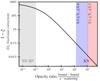 |
Fig. 3. Fractional correction to the estimated luminosity distance from dilution factors, 1 − ξ, as a function of opacity ratio, κb − b/κe−scat. As the opacity ratio is a function of wavelength, we report the integrated Planck mean opacity. When electron-scattering dominates, as in the case of SN IIP (Sim 2017), the photospheric radius inferred from lines will be larger than the thermalisation radius of the blackbody inferred from its flux, thus requiring the introduction of a significant dilution-factor (grey region). However, for neutron-star mergers the bound–bound opacity dominates over electron-scattering, regardless of whether one uses opacities based on lists of known lines (e.g., Tanaka & Hotokezaka 2013) or the higher opacities used in this figure, which are based on more complete theoretically-calculated line-lists (Tanaka et al. 2020). Such dominance of the bound–bound opacity implies negligible corrections to the distance (blue and red hatched region). |
In contrast, for KNe the environment dilution factors are minor. First, the absorption and emission features of the spectrum are explicitly parametrised and fit. Second, the contribution of electron-scattering opacity to the total opacity is expected to be negligible in KN atmospheres, as κb − b is typically several orders of magnitude higher in the UV-optical (Kasen et al. 2013), while the number of free electrons per unit mass is reduced by ≈102 relative to ionised hydrogen. Thus, electron scattering opacity is expected to be less than the r-process line opacity at the relevant wavelengths, and so the dilution effect should be very small, which results in a tight correspondence between thermalisation and photospheric radii. In Tanaka et al. (2020) the Planck mean opacity from bound–bound transitions (at the characteristic temperatures analysed here) ranges from 0.4 to 40 cm2 g−1 for models that are respectively light or heavy r-process dominated. These mean opacities are 130 and 13 000 times larger than the corresponding electron-scattering opacity for NSM ejecta, κe−scat ≈ 3 × 10⁻³ cm2 g−1 (e.g., Eq. (12) in Kasen et al. 2013) and are indicated in the blue and red hatched regions in Fig. 3. Regardless of the exact r-process elementary abundances, dilution-factors are expected to be negligible in KNe.
Another line of reasoning, which illustrates the smaller importance of dilution factors in KNe is the consistent measurements of distance across epochs. When dilution-factors are required to correctly fit the distance such as is the case of SN IIP, the invoked dilution-corrections have to vary across epochs. This is because κe−scat decreases with time (because the temperatures and ionisation-levels decrease), while κb − b increases over photospheric epochs in models (Tanaka & Hotokezaka 2013). For example, the ratio κb − b/κe−scat increases by a factor of 10 from 1.5 to 3.5 days post-merger for the models presented in Bulla et al. (2019). However, while the epochs examined here (in addition to epochs 3, 4, and 5 analysed in Sneppen et al. 2023) probe significantly different phases and characteristic opacities, they still yield consistent measurements of distance. The only physical regime where changing the ratio of opacities drastically does not lead to a shift in distance, is when the bound–bound opacities dominate and ξ ≈ 1.
4.2. The blackbody assumption
It is worth noting that the observed blackbody of the spectrum is difficult to reproduce and explain within current radiative transfer simulations. This is due to the complexities associated with a line-dominated opacity and problems in modelling r-process elements, which have incomplete atomic data and line lists (Gaigalas et al. 2019; Tanaka et al. 2020; Gillanders et al. 2021). For now, therefore, the blackbody origin cannot be derived from first principles, and is instead an empirical assumption based on the close similarity to a blackbody in both luminosity and spectral shape at all wavelengths from the UV to the NIR in the early spectra of AT2017gfo. Therefore, this methodology relies on the ansatz that the emitting plasma really is a blackbody to better than the required accuracy (currently a few percent in the luminosity). This ansatz will be tested in the coming years given ongoing work in improving the relevant atomic data and radiative transfer in kilonova atmospheres (e.g., Domoto et al. 2021; Gaigalas et al. 2019; Gillanders et al. 2022; Flörs 2023). However, the blackbody assumption is not essential to the method, and, as in the spectral-fitting expanding photospheres method (SEAM, Baron et al. 2004), a complete radiative transfer simulation should ultimately be used.
Given the significant light travel time-delays, the rapidly cooling surface and the varying projected velocity of the relativistic Doppler corrections, we note that the different latitudinal parts of the surface are observed with different effective temperatures. This results in a multi-temperature blackbody (i.e., a blackbody convolved over a range of different effective temperatures). However, as shown in Sneppen (2023) for the characteristic velocities and cooling-rates of AT2017gfo these effects cancel and the variations with wavelength remain below 1% over the entire spectral range, suggesting that any angular dependence over the observed surface is negligible.
Even so, the EPM framework can straightforwardly be extended with a modified blackbody framework given any prescribed relation between temperature and time. Using the predicted power-law decay from a large ensemble of r-process isotopes (Metzger et al. 2010; Wu et al. 2019), which is also observed from the fading of the light curves for AT2017gfo (Drout et al. 2017; Waxman et al. 2018), the derived distances remain robust to the assumed cooling rate. In other words, given the functional form
 (5)
(5)
the difference in inferred distance between assuming a constant temperature (α = 0) and the power-law decay inferred from cross-spectra comparisons (α ≈ 0.4 − 0.5) are below 1% (Sneppen 2023).
Furthermore, the wavelength-dependence of opacity and the possibility of a significant radial temperature gradient could imply that different wavelengths probe different radii, and thus temperatures. This radial convolution would again produce a modified blackbody (dependent on the density profile, temperature gradients, and wavelength-dependence of the opacity), which would be broader than a single-temperature blackbody spectrum. However, the spread of temperatures allowed observationally from fits to the kilonova spectra, as calculated in Sneppen (2023), suggests this must be a rather limited effect. As a check on the wavelength-dependence of the blackbody, we fit the UV arm and optical–NIR arms separately in epochs 1 and 2. These yield blackbody temperatures consistent at the level of 2% and 4%, respectively, indicating a consistent single temperature at least from the blue into the near-infrared.
4.3. Flux calibration
The flux calibration of the X-shooter spectra is consistent with coincident photometry from GROND, DECam, EFOSC2, LDSS, Swope, and VIRCAM, as illustrated for Epoch 1 in Fig. 4. Therefore we follow Watson et al. (2019) and Sneppen et al. (2023) and do not artificially scale the spectra to the available photometric data, which have significant internal scatter.
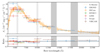 |
Fig. 4. X-shooter spectrum and photometry for the KN AT2017gfo from UV–NIR for observations from 1.35 to 1.45 days after the NS merger GW170817. The dark shaded bars indicate telluric regions; the light shaded bars indicate overlapping noisy regions between the X-shooter UVB, VIS, and NIR arms. The ratio of photometric points to the spectrum (illustrated in the lower panel) shows that while there is significant scatter between photometric points, the normalisation of the spectrum is consistent with the average of the photometric fluxes to within 1%. Data are taken from the literature as follows: GROND and EFOSC2 (Smartt et al. 2017); DECAM (Cowperthwaite et al. 2017); LDSS (Shappee et al. 2017); Swope (Coulter et al. 2017); VIRCAM (Tanvir et al. 2017). |
Nevertheless, we do use the photometric data to ensure our errors are robust. We compute the standard error of the ratio of the photometric fluxes to the synthetic flux from the spectrum integrated over the filter profile for all photometric points (including all observations from GROND, DECam, EFOSC2, LDSS, Swope, and VIRCAM). We add this standard error to the normalisation uncertainty from the fit. In practice, this is implemented by taking the posterior distribution of the normalisation sampled with MCMC and multiplying each instance of the sampling with a random number drawn from a Gaussian distribution with a mean of 1 (as the photometry and spectrum are consistent) and a standard deviation equal to the standard error of the flux calibration. The standard error of the photometric points relative to the X-shooter spectra are 2.5% and 3.8% for epoch 1 and epoch 2, respectively. This method is very cautious; in Sneppen et al. (2023) the errors were increased by the uncertainty on the weighted average between the photometric points and the X-shooter spectrograph, which adds an additional uncertainty of 0.5% and 0.8% on the normalisation for epochs 1 and 2, respectively. For this analysis, we chose the unweighted standard error as coincident photometric points at comparable wavelengths show a low level of discrepancy between different telescopes (see Fig. 4), which suggests that the stated uncertainties in the available photometry may be underestimated.
4.4. Dust extinction
Dust extinction is one of the major uncertainties in SN cosmology and may yet hold some clues to the Hubble tension (e.g., Wojtak & Hjorth 2022). For kilonova distance measurement, we must therefore also carefully consider the level and uncertainty of the extinction. The extinction originates in the Milky Way and potentially in the host galaxy. In the case of AT2017gfo, the Milky Way dust dominates.
4.4.1. Milky Way extinction
In the direction of the host galaxy, the Galactic reddening estimate is E(B − V) = 0.1053 ± 0.0012 based on dust emission data from the IRAS and COBE satellites, calibrated to an extinction measure using SDSS stellar spectra (called the SFD maps; Schlegel et al. 1998; Schlafly & Finkbeiner 2011). This value is consistent with estimates based on Galactic Na D absorption lines (Shappee et al. 2017; Poznanski et al. 2012), though the Na D correlation with dust extinction has large scatter (Poznanski et al. 2011) and is not a useful constraint in this context. The ∼1% uncertainty in E(B − V) quoted above is very small and is an underestimate of the total absolute extinction uncertainty. We address this further here. The dust maps (Planck Collaboration Int. XLVII 2016) calculated using data from the Planck satellite, disentangled from cosmic infrared background anisotropies using the generalized needlet internal linear combination (GNILC) method, and combined with the SFD maps and IRIS maps (Miville-Deschênes & Lagache 2005) is in agreement with the above numbers: the Planck-GNILC data suggest E(B − V) = 0.1068 ± 0.005 along this sightline. The 3D dust maps based on extinction measurements using stellar photometry from stellar photometry of 800 million stars from Pan-STARRS 1 and 2MASS (Green et al. 2018) independently gives E(B − V) = 0.116 ± 0.007 in this direction. None of these Galactic extinction uncertainties would substantially change the uncertainty on the distance (see below) and all these estimates are consistent with each other at the level of 10%. We use E(B − V) = 0.11 which is the weighted average of Green et al. (2018) and Planck Collaboration Int. XLVII (2016), and conservatively use a 15% uncertainty including the absolute uncertainty in this direction. The extinction correction is implemented as laid out in Watson et al. (2019), which assumes the Fitzpatrick (1999), Fitzpatrick et al. (2004) reddening law with RV = 3.1. In addition, we also adopt a 10% uncertainty on the RV, which we propagate throughout the uncertainty estimates of this analysis. This is based on the standard deviation of RV values found along different Milky Way sightlines (Fitzpatrick & Massa 2007; Mörtsell 2013).
4.4.2. Host galaxy extinction
To get an estimate of the likely level of extinction in the host galaxy along this sightline, we estimate the dust surface density at the location of AT2017gfo in its host galaxy and convert it to an extinction estimate as follows. We start with the stellar mass surface density at 2.1 kpc based on the Sérsic model fit by Blanchard et al. (2017), and convert it to a dust surface density using the typical stellar mass-to-dust mass ratio for elliptical galaxies measured by the Herschel Reference Survey, log(MD/M*) = − 5.1 ± 0.1 (Smith et al. 2012). This gives us a surface dust density of 2780 M⊙ kpc−2. Assuming AT2017gfo is in the middle of this dust, we divide by two. We then convert this to an extinction along this line of sight using the gas-to-dust mass ratio for the Milky Way, 90–150 (Magdis et al. 2012; Galametz et al. 2011; Draine et al. 2007), and the relation between gas column density and extinction, NH ∼ 2 × 1021 cm−2 AV (Watson 2011; Bohlin et al. 1978). This returns a value of AV ≃ 0.01. Equally, if we use the conversion from Planck Collaboration Int. XXIX (2016) directly from the dust surface density, ΣMd (i.e., 0.74 × 10⁻⁵ × ΣMd M⊙ kpc−2) we get a similar result. Our estimate is highly uncertain, but small (about 3% of the estimated Milky Way extinction; the redshift effect on the dust extinction curve is negligible at this distance), and also small compared to our uncertainty on the Milky Way extinction, so following Drout et al. (2017) and Watson et al. (2019), we do not correct for reddening from dust within the host galaxy. The lack of observed Na D features in the spectrum at the redshift the host galaxy Shappee et al. (2017) also favors quite a low intrinsic absorption within the host (E(B − V)≲0.03 using the relation of Poznanski et al. 2012). Blanchard et al. (2017) find a similar upper limit for the total dust attenuation of the light of NGC 4993 (AV < 0.11 mag) based on modelling the spectral energy distribution of the whole galaxy, again, consistent with our low estimate. While in this case we find the host galaxy extinction negligible compared to the Milky Way extinction, a better estimate would be useful.
4.4.3. Effect of extinction on the distance estimate
There are two opposing effects on the inferred luminosity distance if a significant amount of dust is not accounted for. First, attenuation of the light would make the object appear fainter, which would lead us to infer a greater distance. Second, the reddening effect of the dust extinction would make the observed blackbody appear cooler (i.e., the kilonova would be inferred from the fit to be intrinsically less luminous, and thus closer to the observer). These two effects largely counteract each other, with the apparent cooling effect being slightly dominant for the wavelengths and temperatures of AT2017gfo at the epochs analysed here. Thus, the competing effects of biasing the apparent temperature and luminosity mean that the uncertainty in the dust extinction level we infer here only corresponds to around a 1.5% fractional uncertainty in the distance.
Overall, finding a more accurate way to measure host galaxy extinction for future events may be important, at least in some cases, if we are to use kilonovae to estimate H0 to high precision. In general, however, kilonovae occur in less dusty environments than SNe, so the extinction corrections will typically be smaller than for most SNe. Furthermore, it is likely that on average, future KNe will have lower Galactic extinction, with the median Galactic extinction values from X-ray-selected GRB samples being around AV = 0.1 − 0.2 (e.g., Watson 2011).
4.5. Evolving spectral line emission
While the earliest epochs of AT2017gfo are well approximated by a blackbody spectrum (Malesani et al. 2017; Drout et al. 2017; Shappee et al. 2017), over time, the spectrum increasingly deviates from a blackbody with more numerous and progressively stronger spectral components. Broad excess emission is observed at wavelengths of around 1.5 μm and 2 μm; there is an emission feature at ∼1.4 μm within the telluric region, clearly observed in the Hubble Space Telescope spectra from the fifth and tenth days post-merger (Tanvir et al. 2017). The derived constraints are robust at early times, whether one includes these components in a parametrised fashion, excludes the spectral regions containing these components, or indeed neglects modelling these features altogether (see Fig. 5). Thus, while the modelling of later epochs may be affected by whether and how these features are accounted for, the constraints from the earliest epochs are little affected by these emerging spectral components. For the constraints presented in this paper, we include Gaussian emission lines as nuisance parameters to explicitly parametrise the observed emission components at 1.5 μm and 2 μm.
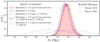 |
Fig. 5. Posterior probability distributions of luminosity distances for the first epoch spectrum with and without modelling of different emission features. This shows the size of effects related to the choice of how the continuum and lines are modelled. The canonical model (red) is a blackbody continuum with Sr+ elementary supernova P Cygni lines and Gaussian emission lines at 1.5 μm and 2 μm. The green histogram shows the effect of limiting the analysis to wavelengths below 1300 nm and using only a blackbody continuum with Sr+ P Cygni, which avoids the need to include the 1.5 μm and 2 μm lines in the model. Very similar distances are found fitting the full dataset with only a blackbody and the Sr+ P Cygni lines (blue) or only fitting the absorption wavelengths of the P Cygni (purple) (i.e., excluding the P Cygni emission wavelengths, 1 μm < λ < 1.3 μm, from the fit). Lastly, the distance is robust to the lower wavelength cutoff as seen by fitting the canonical model to wavelengths λ > 330 nm (red) or λ > 400 nm (yellow). The fitting result is therefore very robust to the details of how the fit is performed and what data are included. Distances inferred from the cosmological redshift are also plotted for H0 = 67.36 ± 0.54 (Planck Collaboration VI 2020) (dotted purple) and H0 = 73.03 ± 1.04 (Riess et al. 2022) (dotted blue). |
Thus, in constraining the continuum we can use the broad wavelength coverage from the UV at 330 nm to the NIR at 2250 nm (excluding the telluric regions and noisy regions between UV, optical, and NIR arms). The analysis is not very sensitive to the specific wavelength range used (see Fig. 5). Naturally, the constraining power decreases given a more limited wavelength range. The blue and visible flux is important for fitting the blackbody peak (and in extension the blackbody temperature and normalisation); however, for reasonable choices of the short wavelength cutoff (i.e., 330 nm–400 nm) the derived distance remains highly consistent.
4.6. Line blending
The identification of the 1 μm P Cygni feature as being primarily due to Sr+ is consistently recovered in radiative transfer simulations (Watson et al. 2019; Domoto et al. 2021; Gillanders et al. 2022) as (1) strontium is a highly abundant element in both the r-process abundance of the sun and in nucleosynthesis models (being near the first r-process peak), (2) Sr+ has three strong lines at the observed rest-wavelength, and (3) the low-lying energy levels are easily accessible in local thermodynamic equilibrium for the characteristic temperatures in the kilonova atmosphere. However, a potential concern is that blending with other as-yet-unrecognised lines not in the available line lists could bias the inferred properties from the Sr+ P Cygni profile. As discussed in Sneppen et al. (2023), such a significant biasing line is not observationally required by the data and would be unlikely to produce the very consistent distances measured across multiple epochs. Furthermore, the velocity derived from Sr+ is consistent with the velocity stratification from the detection of a newly discovered yttrium P Cygni feature at ∼0.76 μm discovered in later epoch spectra (Sneppen & Watson 2023). Thus, any potential line blending bias would have to act coincidentally to reproduce consistent distance estimates and symmetry not merely across epochs, but also across different lines probing different wavelengths.
To obtain a consistent distance across different epochs would require that the blending lines matched the Sr+ lines in strength over time, despite the major changes in density and temperature (as well as possible composition) that we observe at each epoch. In addition, this requires the blending lines to mimic a Sr+ P Cygni profile, coherently shifting in wavelength and receding deeper within the ejecta at exactly the rate predicted by the blackbody continuum. On the basis of this argument, it seems unlikely that line blending is substantially biasing the determined photospheric velocities, although in principle it cannot be excluded, and therefore remains a systematic uncertainty. This effect could be quantified with a full radiative transfer model with a complete atomic dataset for the relevant elements.
4.7. Reverberation effects
A significant issue with current P Cygni codes is the lack of reverberation effects which current models do not include. Reverberation effects happen because the strength of the observed lines are dynamically evolving, and due to different light travel-times, the flux from different wavelengths in the line were emitted at different times. In conjunction, these imply that the constraints may be improved with a full 3D (or at least 2D) radiative transfer model. Modelling these higher order effects are outside the scope of the simplicity of our current framework and this initial analysis, but we note that reproducing kilonova spectra and their temporal evolution within an ensemble of self-consistent radiative transfer models could improve the confidence in, and the quality of, the constraints compared to these preliminary results.
4.8. Measuring the sphericity
A high degree of sphericity is indicated by the line shape and the consistently spherical measurement from the EPM framework across epochs. First, the characteristic fractional uncertainty on geometry from the line shape fitting is of the order of 1%. Second, the 2% spread in the statistically independent measurements of the sphericity index σΥ from epochs 1, 2, and 3 from the EPM analysis in Sneppen et al. (2023) provides an estimate of the upper bound on the internal uncertainty of this measurement. However, there is a slight evolution of both EPM and line shape constraints in the same direction and of comparable magnitude over time, hinting that the initially spherical ejecta geometry becomes slightly and increasingly prolate. While we account for this very mild monotonically increasing prolateness from the line shape, the majority of the observed scatter in distance estimates might still be caused by an underlying evolution in the geometry if it is not fully accounted for. That is because the EPM distance inferred from Eq. (3) becomes slightly and monotonically larger in later epochs (Sneppen et al. 2023) in the same way as the prolateness inferred from the line shape.
Additional constraints on the kilonova’s asymmetry from spectropolarimetry at 1.46 days are consistent with this spherical geometry, with the observed low degree of polarisation being consistent with intrinsically unpolarised emission scattered by Galactic dust (Covino et al. 2017; Bulla et al. 2019). This indicates a symmetrical geometry of the emitting region, with a very loose constraint on the viewing angle of 65° of the pole. While these measurements are not very constraining, spectropolarimetry could provide useful independent constraints of geometry and sphericity for future kilonovae.
For this analysis, we propagate the geometrical uncertainty from the line shape in Sneppen et al. (2023) into the final cosmological constraint. However, as noted, the geometrical constraints from line shapes may be affected by reverberation effects or blending lines, so these constraints should be considered preliminary to such improvements in radiative transfer modelling of KNe. Nevertheless, given the dominance of the peculiar velocity uncertainty, a somewhat looser constraint on sphericity would not drastically impact the H0 error budget, as indicated in Fig. 6. It would require an increase of a factor of several in the uncertainty in sphericity to make it comparable to the peculiar velocity uncertainty for AT2017gfo. Thus, despite the degeneracy in line shape fitting between geometry constraints and viewing inclination angle, moderately looser inclination constraints, such as that provided by using only the radio jet θinc = 21 ± 7 (Mooley et al. 2018), will not significantly increase the error budget. Inclination angle observations are currently necessary for strong line shape constraints. Unfortunately, a significant fraction of expected KNe may have no jet observations (Colombo et al. 2022) we therefore cannot rely on them having well-constrained geometries. On the other hand, if a very high degree of sphericity proves to be a common feature of KNe, this may not be problematic. With improved numerical simulations, which can consistently explain and reproduce the observed geometry of future KNe, the deviation from sphericity and spread of geometry within such simulations can also be propagated within this framework.
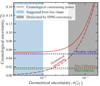 |
Fig. 6. Cosmological constraints attainable for AT2017gfo as a function of the constraints on the ejecta geometry. The uncertainty associated with peculiar velocity modelling dominates for a well-constrained geometry, while a poorly constrained shape would dominate the error-budget when the fractional uncertainty exceeds 5%. The small scatter across the independent datasets from days 1.4–3.4 post-merger (Sneppen et al. 2023) puts an upper bound on the statistical uncertainty on the geometry of a few percent (indicated with grey shading). Additionally, prior line shape constraints (blue shading) suggest percent-precision geometrical constraints may be attainable (Sneppen et al. 2023). Thus, both the EPM consistency and line shape analysis suggest, that AT2017gfo is in the regime where peculiar velocity modelling is the dominant uncertainty. |
4.9. Continuum relativistic and time-delay correction
The systematic effects and uncertainties discussed previously are important at the percent level for constraining distances, which for any H0 constraints are well below the 5% fractional uncertainty in modelling the peculiar velocity. Including the full relativistic and time-delay corrections on the continuum luminosity matters at the ∼10% level for the characteristic velocity of the early kilonova ejecta. Thus, it is important to get this right, and in the following we discuss the time-delay and relativistic correction f(β) used in Eq. (1).
First, the significant time-delay of the mildly relativistic velocities induces a geometrical effect. In order to be observed at the same time, light arriving from the limb of the ejecta must have been emitted earlier than the light from the nearest front, at a time when the photosphere had a smaller surface area. As first derived in Rees (1967), this defines a surface of equal arrival time rph(μ)/rph(μ = 1) = (1 − β)/(1 − βμ), where μ = cos(θ), with θ being the angle between expansion and the line of sight.
Second, the specific intensity is a blackbody B(λ′,T′) with temperature T′ at wavelength λ′ in the co-moving frame of the ejecta, which in the observed frame is inferred as a blackbody B(λ, T) with an observed temperature T and wavelength λ. The relationship between emitted and observed temperature T(μ) = δ(μ)T′ is given by the relativistic Doppler correction δ(μ) = (Γ(1−βμ))−1 (Ghisellini & Processes 2013). Here the Lorentz-factor Γ represents the relativistic time dilation, while the latter is the Doppler correction, which depends on the projected velocity along the line of sight μ. We note that this means that it is a mathematical property of a blackbody in bulk motion, and that while the relativistic transformations boost the observed luminosity, this is exactly matched by a higher observed temperature.
However, as the ejecta’s projected velocity varies across different surface elements (from head-on expansion, μ = 1, to orthogonal, μ = 0), so too will the Doppler correction vary. This results in a second-order correction, where a convolution of relativistic Doppler corrections incoherently shift the spectrum. The deviation generally depends on the spectral shape, but for this analysis the variations with wavelength are below 1% over the entire spectral range (Sneppen 2023). Thus, for the mildly relativistic velocities of relevance here, the luminosity-weighted spectrum remains largely well described by a single blackbody B(λ, Teff), so the relativistic correction is not central for the cosmological constraints.
In conjunction, these transformations yield an observed luminosity (Sneppen et al. 2023)
![Mathematical equation: $$ \begin{aligned} L_{\lambda }^\mathrm{BB}&= \int I_\lambda \mu \ \mathrm{d}\mu \ \mathrm{d}\phi \ \mathrm{d}A \\&= 2 \pi \int _\beta ^1 \delta (\mu )^5 B(\lambda \prime , T\prime ) \left(4 \pi R_{\rm ph}^2 \left(\frac{1-\beta }{1-\beta \mu }\right)^2 \right) \mu \mathrm{d}\mu \\&= 4 \pi R_{\rm ph}^2 \left[2 \pi \int _\beta ^1 B(\lambda , T(\mu )) \left(\frac{1-\beta }{1-\beta \mu }\right)^2 \mu \mathrm{d}\mu \right] \\&= 4 \pi R_{\rm ph}^2 \left[f(\beta )\;B(\lambda ,T_{\rm eff})\right], \end{aligned} $$](/articles/aa/full_html/2023/10/aa46306-23/aa46306-23-eq9.gif)
where f(β) represents the relativistic and time-delay correction drawn in Fig. 7. The limits of integration follow from the relativistic transformation of angles (see Sadun & Sadun 1991).
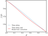 |
Fig. 7. Time-delay and relativistic correction f(β) as a function of expansion velocity β. For non-relativistic velocities the integral over solid angle reduces to π, but decreases at greater velocities due to the geometrical effect in Rees (1967). The blue dashed line indicates the geometrical correction only, while the red line includes the full correction of both time-delays and relativity. In the highly relativistic limit the time-delay effect implies the observed surface area approaches 0, as only the ejecta expanding towards the line of sight is visible. |
4.10. Line relativistic correction
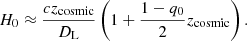
The standard P Cygni prescription codes often used in modelling lines, including the elementary supernova model, are inherently non-relativistic. It assumes an isotropic source function, an optical depth τ which is symmetric across angles, μ = cos(θ), and a planar resonance surface. These assumptions are valid in the co-moving frame of the ejecta, but are problematic in the observer’s frame for a relativistic expansion, where aberration of angles produces an anisotropic optical depth and source function, while time dilation results in a convex surface of equal frequency. Therefore to determine the magnitude of these relativistic corrections in the mildly relativistic regime of AT2017gfo, we have also used the relativistic corrections for P Cygni profiles derived in Hutsemekers & Surdej (1990). The derived relativistic transformations are as follows. Firstly, the source function Sobs in the observer frame is beamed compared to the co-moving frame: Sobs = Sco δ(μ)2 (for the relativistic transformation of the initial specific intensity I, see Sect. 4.9). Secondly, given homologous expansion, the optical depth in the observer frame, τobs(r, μ), is related to the optical depth in the co-moving frame τco(r) as
![Mathematical equation: $$ \begin{aligned} \tau _{\rm obs}(r,\mu ) = \tau _{\rm co}(r)\,\left|\frac{(1-\mu \beta )^2}{(1-\beta ) [ \mu (\mu - \beta )+(1-\mu ^2)(1-\beta ^2)]} \right|.\end{aligned} $$](/articles/aa/full_html/2023/10/aa46306-23/aa46306-23-eq10.gif) (6)
(6)
Thirdly, the surface of equal frequency ν is shifted relative to the rest frequency of the line ν0 by the relativistic Doppler correction, so it must satisfy the relation
![Mathematical equation: $$ \begin{aligned} \frac{\nu _0}{\nu } = \Gamma (r) [1-\mu \beta (r)], \end{aligned} $$](/articles/aa/full_html/2023/10/aa46306-23/aa46306-23-eq11.gif) (7)
(7)
which for any frequency ν can be solved for position (r, μ).
These relativistic corrections are relatively minor, yielding a slight systematic increase in the inferred distance with respect to the non-relativistic P Cygni code, but within the 90% error region (Fig. 8). Given the peculiar velocity uncertainties for AT2017gfo, these relativistic corrections are minor for the current cosmological measurements, though they do affect the distance estimate by about 2%. While we do not apply the correction here as it would be inconsistent with our line shape modelling from Sneppen et al. (2023), for future work these effects should be included.
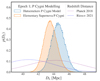 |
Fig. 8. Effect of relativistic correction on posterior probability distributions of luminosity distances for the first epoch spectrum. The elementary supernova model is shown in orange and the same model including the relativistic corrections of Hutsemekers & Surdej (1990) is shown in light blue. For the mildly relativistic regime these systematic corrections are within the uncertainties of the distance. Cosmological redshift distances are also plotted for H0 = 67.36 ± 0.54 (Planck Collaboration VI 2020) (dotted purple) and H0 = 73.03 ± 1.04 (Riess et al. 2022) (dotted blue). |
4.11. Summary of systematics and corrections
We propagated the uncertainties associated with dust extinction, flux calibration, and sphericity into our constraints on the distance (see Table 1). The overall derived distance is robust to the later-emerging emission features and to the relativistic and time-delay corrections to the continuum and P Cygni profile. The model-dependent dilution factors necessary for EPM analysis of core-collapse supernovae are expected to be and appear to be negligible in the r-process-dominated atmospheres of kilonovae. However, the methodological framework presented here, while having the virtue of simplicity, does not include a full 3D code that models the complexities of the radiative transfer self-consistently or reverberation effects. For now, we leave these higher order complexities for future simulation-based analysis. We note that while the blackbody nature of the continuum has so far proven challenging to reproduce in radiative transfer models from first principles, it remains an observationally motivated ansatz in this analysis.
Characteristic contributions to the error budget for the measurement of the Hubble constant with AT2017gfo.
5. Expected constraints with future detections
Ultimately, the analysis of the kilonova AT2017gfo cannot yield an estimate of H0 decisive to the current Hubble tension due to the large peculiar velocity uncertainty of NGC 4993. However, with additional high-quality kilonova observations expected from the upcoming O4 and O5 runs using the Advanced LIGO, Virgo and KAGRA (HLVK) network, significantly tighter constraints are expected for a few key reasons (Chen et al. 2018). First, with larger sample size the statistical uncertainty will decrease, with the random direction of peculiar velocities averaging out. Second, due to increased GW sensitivity, future kilonova are expected mostly to lie at greater distances, where the fractional impact of peculiar velocity uncertainties are likely to be smaller. Ongoing peculiar velocity surveys will improve the accuracy of peculiar velocity models (Kim & Linder 2020), likely for more distant galaxies as well. Conversely, larger distances will result in fainter optical counterparts with correspondingly lower signal-to-noise ratio (S/N) spectra, though for AT2017gfo spectral S/N is not the limiting factor in the precision of the constraints. In the following, we provide a rough estimate on the potential H0 constraints attainable with this method for AT2017gfo-like kilonovae. It is probable that a significant fraction of future kilonovae will be different to AT2017gfo (Gompertz et al. 2018; Rossi et al. 2020; Kawaguchi et al. 2020; Korobkin et al. 2021), though in exactly what parameters and how they relate to their use as a H0 probe is unclear. Whether the geometry of AT2017gfo is characteristic of kilonovae in general is unknown, for example, and theoretically we may expect a certain range of geometries depending on the binary parameters. Future detections of even aspherical kilonova ejecta can still be used within the EPM framework if the geometry is well constrained. Constraints on geometries can be obtained with spectropolarimetry, EPM, or line shape measurements with inclination angle constraints, complemented by numerical simulations. It is also possible that certain kilonova sub-types may be spherical, and these can be identified with such measurements of a large enough population.
To quantify the statistical distance uncertainty the EPM framework will yield for future detections at greater distances, we generate and fit simulated spectra at variable S/N based on the AT2017gfo data. In Fig. 9 we indicate the fractional uncertainty on luminosity distance obtained from a single object with an identical intrinsic luminosity as the first epoch spectrum, but placed at greater distance. Thus, the mock object at 43 Mpc has an identical S/N valute to the observed first epoch spectrum of AT2017gfo. Naturally, the statistical uncertainty of the fit increases monotonically, reaching a fractional uncertainty of ≈1% for a detection at 150 Mpc.
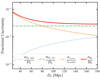 |
Fig. 9. Fractional uncertainty on H0 (red line) for a future kilonova detection with similar intrinsic luminosity, systematic uncertainties, and peculiar velocity uncertainty as AT2017gfo. The dominant contribution for objects at DL < 100 Mpc is the uncertainty from peculiar velocities (dashed orange line) assuming the total peculiar velocity uncertainty is independent of the distance. The statistical uncertainty on the luminosity distance for mock spectra objects with the same intrinsic luminosity as the first X-shooter epoch increases with distance (blue dotted lines). The systematic uncertainties in distance from sphericity constraints, flux calibration, and dust extinction are considered to be independent of the source distance. |
Additionally, the systematic distance uncertainties associated with flux calibration, dust extinction, or the degree of asphericity contribute to the error budget. This is laid out in Table 1 for AT2017gfo specifically. For the more general case, the relative contribution of each of these is set by the favorability of observations; for instance, the quality of coincident photometry for flux calibration, the dust extinction toward the object, or the power of line shape (or spectropolarimetry) analysis to constrain the asphericity. For AT2017gfo these yield a fractional distance uncertainty of around 2% with the dominant systematic uncertainties being the constraint on the ejecta sphericity and the flux calibration, which are largely independent of distance. Thus, for future kilonova detections at greater distance, the fractional uncertainty due to systematics is assumed in this simple model to be unchanged (see Fig. 9).
In contrast, to first approximation the typical peculiar velocity uncertainty is largely independent of distance, so the fractional uncertainty is assumed to decrease as  . We note that this is a somewhat optimistic assumption as the peculiar velocity reconstruction may deteriorate slightly for distances greater than 100 Mpc. Secondly, we assume the total peculiar velocity uncertainty of NGC 4993 is representative of future kilonova host galaxies. Carrick et al. (2015) predicted that the typical error when modelling the peculiar velocity field within approximately 250 Mpc is around 150 km s−1. Thus, the NGC 4993 peculiar velocity error, 130 km s−1, is quite typical, in no way particularly large or small. Subject to these two assumptions, the peculiar velocities remain the dominant uncertainty up to DL ≈ 80 Mpc, as illustrated in Fig. 9. An individual kilonova observation at DL ≈ 150 Mpc with both GW signatures and high S/N spectral follow-up could alone yield an estimate of H0 to ∼3% precision.
The largest unknown in forecasting future constraint capabilities for HLVK runs O4 and O5 is estimating the number of well-localised binary neutron star (BNS) mergers (or at least, those similar to AT2017gfo). We do not comment on this issue here. Instead in Table 2 we show the expected constraint on H0 attainable with one, five, and ten kilonovae with similar intrinsic luminosity and peculiar velocity to AT2017gfo. These detections are assumed to be uniformly distributed within the observable volume up to 150 Mpc. The typical BNS merger for this volume is located at  Mpc. It is worth noting that within these distances, the cosmic variance for any local measurement of H0 is at the one percent level (Wojtak et al. 2014), which sets a lower bound on the cosmological precision attainable from averaging over local objects. Nevertheless, these results suggest that applying EPM to kilonovae may yield percent-precision H0 constraints given the current detection sensitivities and a handful of detections. For the nearest kilonova observations, at smaller or similar distances to NGC 4993, this framework can be complemented by, and even incorporated within, the cosmological distance ladder, for example by making Cepheid observations within the host galaxies and comparing them with the inferred distance.
Future number of kilonovae detected with GW and optical counterparts vs. the expected fractional constraint attainable on H0.
6. Conclusions
We have shown in this paper how spectral analysis of well-observed kilonovae can be used to measure the expansion rate of the universe to a precision of a few percent, with low systematic uncertainty. Using AT2017gfo as an example, we have examined the dominant statistical and systematic uncertainties and derived a preliminary value of the Hubble constant accurate to about 5%, dominated by the host galaxy peculiar velocity. While we believe that the important systematic effects have been considered, we reiterate that the value of H0 we present here is preliminary and may be subject to significant change once a full 3D radiative transfer simulation can accurately capture effects such as the light travel time reverberation and the true nature of the kilonova atmosphere, which are not accounted for in our modelling. We also show that a sample of a handful of kilonovae with luminosity and characteristics similar to AT2017gfo, such as may be detected in the upcoming HLVK runs O4 and O5, and well observed spectroscopically, could be made to yield a value of H0 accurate to about 1%.
We adapt Ulrich Noebauer’s pcygni_profile.py, https://github.com/unoebauer/public-astro-tools
Acknowledgments
We thank Jonathan Selsing, Stuart Sim and Ehud Nakar for useful discussions and feedback. We also wish to express gratitude to Brandon Hensley, Bruce Draine, Douglas Finkbeiner, Anja Andersen, and Adam Riess for providing comment to improve the discussion on uncertainties from dust extinction. The Cosmic Dawn Center is funded by the Danish National Research Foundation under grant number 140. AB and OJ acknowledge support by the European Research Council (ERC) under the European Union’s Horizon 2020 research and innovation programme under grant agreement No. 759253, by the Deutsche Forschungsgemeinschaft – Project-ID 279384907 – SFB 1245, and by the State of Hesse within the Cluster Project ELEMENTS. RW was supported by a grant from VILLUM FONDEN (project number 16599)
References
- Abbott, B. P., Abbott, R., Abbott, T. D., et al. 2017, Nature, 551, 85 [Google Scholar]
- Arcavi, I. 2018, ApJ, 855, L23 [NASA ADS] [CrossRef] [Google Scholar]
- Baade, W. 1926, Astron. Nachr., 228, 359 [NASA ADS] [CrossRef] [Google Scholar]
- Baron, E., Nugent, P. E., Branch, D., & Hauschildt, P. H. 2004, ApJ, 616, L91 [NASA ADS] [CrossRef] [Google Scholar]
- Birrer, S., Shajib, A., Galan, A., et al. 2020, A&A, 643, A165 [NASA ADS] [CrossRef] [EDP Sciences] [Google Scholar]
- Blanchard, P. K., Nicholl, M., Berger, E., et al. 2017, ApJ, 848, L22 [NASA ADS] [CrossRef] [Google Scholar]
- Bohlin, R. C., Savage, B. D., & Drake, J. F. 1978, ApJ, 224, 132 [Google Scholar]
- Bulla, M., Covino, S., Kyutoku, K., et al. 2019, Nat. Astron., 3, 99 [Google Scholar]
- Cantiello, M., Jensen, J. B., Blakeslee, J. P., et al. 2018, ApJ, 854, L31 [Google Scholar]
- Carrick, J., Turnbull, S. J., Lavaux, G., & Hudson, M. J. 2015, MNRAS, 450, 317 [Google Scholar]
- Chen, H.-Y., Fishbach, M., & Holz, D. E. 2018, Nature, 562, 545 [Google Scholar]
- Collins, C. E., Bauswein, A., Sim, S. A., et al. 2023, MNRAS, 521, 1858 [NASA ADS] [CrossRef] [Google Scholar]
- Colombo, A., Salafia, O. S., Gabrielli, F., et al. 2022, ApJ, 937, 79 [NASA ADS] [CrossRef] [Google Scholar]
- Coughlin, M. W., Dietrich, T., Heinzel, J., et al. 2020, Phys. Rev. Res., 2, 022006 [NASA ADS] [CrossRef] [Google Scholar]
- Coulter, D. A., Kilpatrick, C. D., Siebert, M. R., et al. 2017, Science, 358, 1556 [NASA ADS] [CrossRef] [Google Scholar]
- Covino, S., Wiersema, K., Fan, Y. Z., et al. 2017, Nat. Astron., 1, 791 [NASA ADS] [CrossRef] [Google Scholar]
- Cowperthwaite, P. S., Berger, E., Villar, V. A., et al. 2017, ApJ, 848, L17 [CrossRef] [Google Scholar]
- Dessart, L., & Hillier, D. J. 2005, A&A, 439, 671 [NASA ADS] [CrossRef] [EDP Sciences] [Google Scholar]
- Dessart, L., Hillier, D. J., Woosley, S., et al. 2015, MNRAS, 453, 2189 [NASA ADS] [CrossRef] [Google Scholar]
- Doctor, Z. 2020, ApJ, 892, L16 [CrossRef] [Google Scholar]
- Domínguez, A., Wojtak, R., Finke, J., et al. 2019, ApJ, 885, 137 [Google Scholar]
- Domoto, N., Tanaka, M., Wanajo, S., & Kawaguchi, K. 2021, ApJ, 913, 26 [NASA ADS] [CrossRef] [Google Scholar]
- Draine, B. T., Dale, D. A., Bendo, G., et al. 2007, ApJ, 663, 866 [NASA ADS] [CrossRef] [Google Scholar]
- Drout, M. R., Piro, A. L., Shappee, B. J., et al. 2017, Science, 358, 1570 [NASA ADS] [CrossRef] [Google Scholar]
- Eastman, R. G., Schmidt, B. P., & Kirshner, R. 1996, ApJ, 466, 911 [NASA ADS] [CrossRef] [Google Scholar]
- Efstathiou, G. 2020, arXiv e-prints [arXiv:2007.10716] [Google Scholar]
- Fitzpatrick, E. L. 1999, PASP, 111, 63 [Google Scholar]
- Fitzpatrick, E. L. 2004, in Astrophysics of Dust, eds. A. N. Witt, G. C. Clayton, & B. T. Draine, ASP Conf. Ser., 309, 33 [NASA ADS] [Google Scholar]
- Fitzpatrick, E. L., & Massa, D. 2007, ApJ, 663, 320 [Google Scholar]
- Flörs, A., Silva, R. F., Deprince, J., et al. 2023, MNRAS, 524, 3083 [CrossRef] [Google Scholar]
- Fong, W., & Berger, E. 2013, ApJ, 776, 18 [NASA ADS] [CrossRef] [Google Scholar]
- Gaigalas, G., Kato, D., Rynkun, P., Radžiūtė, L., & Tanaka, M. 2019, ApJS, 240, 29 [NASA ADS] [CrossRef] [Google Scholar]
- Galametz, M., Madden, S. C., Galliano, F., Hony, S., Bendo, G. J., & Sauvage, M. 2011, A&A, 532, A56 [NASA ADS] [CrossRef] [EDP Sciences] [Google Scholar]
- Ghisellini, G. 2013, Radiative Processes in High Energy Astrophysics, 873 [Google Scholar]
- Gillanders, J. H., McCann, M., Sim, S. A., Smartt, S. J., & Ballance, C. P. 2021, MNRAS, 506, 3560 [NASA ADS] [CrossRef] [Google Scholar]
- Gillanders, J. H., Smartt, S. J., Sim, S. A., Bauswein, A., & Goriely, S. 2022, MNRAS, 515, 631 [NASA ADS] [CrossRef] [Google Scholar]
- Gompertz, B. P., Levan, A. J., Tanvir, N. R., et al. 2018, ApJ, 860, 62 [NASA ADS] [CrossRef] [Google Scholar]
- Green, G. M., Schlafly, E. F., Finkbeiner, D., et al. 2018, MNRAS, 478, 651 [Google Scholar]
- Hershkowitz, S., Linder, E., & Wagoner, R. V. 1986, ApJ, 303, 800 [CrossRef] [Google Scholar]
- Hjorth, J., Levan, A. J., Tanvir, N. R., et al. 2017, ApJ, 848, L31 [NASA ADS] [CrossRef] [Google Scholar]
- Hoeflich, P., Wheeler, J. C., Hines, D. C., & Trammell, S. R. 1996, ApJ, 459, 307 [Google Scholar]
- Hönig, S. F., Watson, D., Kishimoto, M., & Hjorth, J. 2014, Nature, 515, 528 [CrossRef] [Google Scholar]
- Hotokezaka, K., Nakar, E., Gottlieb, O., et al. 2019, Nat. Astron., 3, 940 [NASA ADS] [CrossRef] [Google Scholar]
- Howlett, C., & Davis, T. M. 2020, MNRAS, 492, 3803 [Google Scholar]
- Hutsemekers, D., & Surdej, J. 1990, ApJ, 361, 367 [CrossRef] [Google Scholar]
- Jasche, J., & Lavaux, G. 2019, A&A, 625, A64 [NASA ADS] [CrossRef] [EDP Sciences] [Google Scholar]
- Jeffery, D. J., & Branch, D. 1990, in Supernovae, Jerusalem Winter School for Theoretical Physics, eds. J. C. Wheeler, T. Piran, & S. Weinberg, 6, 149 [NASA ADS] [Google Scholar]
- Jones, D. O., Riess, A. G., Scolnic, D. M., et al. 2018, ApJ, 867, 108 [NASA ADS] [CrossRef] [Google Scholar]
- Just, O., Vijayan, V., Xiong, Z., et al. 2023, ApJ, 951, L12 [NASA ADS] [CrossRef] [Google Scholar]
- Kamionkowski, M., & Riess, A. G. 2022, arXiv e-prints [arXiv:2211.04492] [Google Scholar]
- Kasen, D., Badnell, N. R., & Barnes, J. 2013, ApJ, 774, 25 [NASA ADS] [CrossRef] [Google Scholar]
- Kasen, D., Fernández, R., & Metzger, B. D. 2015, MNRAS, 450, 1777 [NASA ADS] [CrossRef] [Google Scholar]
- Kawaguchi, K., Shibata, M., & Tanaka, M. 2020, ApJ, 889, 171 [NASA ADS] [CrossRef] [Google Scholar]
- Kim, A. G., & Linder, E. V. 2020, Phys. Rev. D, 101, 023516 [NASA ADS] [CrossRef] [Google Scholar]
- Kirshner, R. P., & Kwan, J. 1974, ApJ, 193, 27 [NASA ADS] [CrossRef] [Google Scholar]
- Korobkin, O., Wollaeger, R. T., Fryer, C. L., et al. 2021, ApJ, 910, 116 [NASA ADS] [CrossRef] [Google Scholar]
- Magdis, G. E., Rigopoulou, D., Helou, G., et al. 2012, ApJ, 760, 6 [NASA ADS] [CrossRef] [Google Scholar]
- Malesani, D., Watson, D., & Hjorth, J. 2017, GRB Coordinates Network, 21577, 1 [NASA ADS] [Google Scholar]
- Martin, D., Perego, A., Arcones, A., et al. 2015, ApJ, 813, 2 [NASA ADS] [CrossRef] [Google Scholar]
- Metzger, B. D., Martínez-Pinedo, G., Darbha, S., et al. 2010, MNRAS, 406, 2650 [NASA ADS] [CrossRef] [Google Scholar]
- Miville-Deschênes, M.-A., & Lagache, G. 2005, ApJS, 157, 302 [Google Scholar]
- Mooley, K. P., Deller, A. T., Gottlieb, O., et al. 2018, Nature, 561, 355 [Google Scholar]
- Mooley, K. P., Anderson, J., & Lu, W. 2022, Nature, 610, 273 [NASA ADS] [CrossRef] [Google Scholar]
- Mörtsell, E. 2013, A&A, 550, A80 [NASA ADS] [CrossRef] [EDP Sciences] [Google Scholar]
- Mörtsell, E., Goobar, A., Johansson, J., & Dhawan, S. 2022, ApJ, 933, 212 [CrossRef] [Google Scholar]
- Mukherjee, S., Lavaux, G., Bouchet, F. R., et al. 2021, A&A, 646, A65 [NASA ADS] [CrossRef] [EDP Sciences] [Google Scholar]
- Nicholl, M., Berger, E., Kasen, D., et al. 2017, ApJ, 848, L18 [NASA ADS] [CrossRef] [Google Scholar]
- Nicolaou, C., Lahav, O., Lemos, P., Hartley, W., & Braden, J. 2020, MNRAS, 495, 90 [Google Scholar]
- Pesce, D. W., Braatz, J. A., Reid, M. J., et al. 2020, ApJ, 891, L1 [Google Scholar]
- Pian, E., d’Avanzo, P., Benetti, S., et al. 2017, Nature, 551, 67 [NASA ADS] [CrossRef] [Google Scholar]
- Planck Collaboration VI. 2020, A&A, 641, A6 [NASA ADS] [CrossRef] [EDP Sciences] [Google Scholar]
- Planck Collaboration Int. XXIX. 2016, A&A, 586, A132 [NASA ADS] [CrossRef] [EDP Sciences] [Google Scholar]
- Planck Collaboration Int. XLVIII. 2016, A&A, 596, A109 [NASA ADS] [CrossRef] [EDP Sciences] [Google Scholar]
- Poulin, V., Smith, T. L., Karwal, T., & Kamionkowski, M. 2019, Phys. Rev. Lett., 122, 221301 [Google Scholar]
- Poznanski, D., Ganeshalingam, M., Silverman, J. M., & Filippenko, A. V. 2011, MNRAS, 415, L81 [NASA ADS] [CrossRef] [Google Scholar]
- Poznanski, D., Prochaska, J. X., & Bloom, J. S. 2012, MNRAS, 426, 1465 [Google Scholar]
- Rees, M. J. 1967, MNRAS, 135, 345 [Google Scholar]
- Riess, A. G., Yuan, W., Macri, L. M., et al. 2022, ApJ, 934, L7 [NASA ADS] [CrossRef] [Google Scholar]
- Rigault, M., Brinnel, V., Aldering, G., et al. 2020, A&A, 644, A176 [NASA ADS] [CrossRef] [EDP Sciences] [Google Scholar]
- Rossi, A., Stratta, G., Maiorano, E., et al. 2020, MNRAS, 493, 3379 [CrossRef] [Google Scholar]
- Rosswog, S., Korobkin, O., Arcones, A., Thielemann, F. K., & Piran, T. 2014, MNRAS, 439, 744 [NASA ADS] [CrossRef] [Google Scholar]
- Sadun, A. C., & Sadun, L. A. 1991, Ap&SS, 185, 21 [CrossRef] [Google Scholar]
- Schlafly, E. F., & Finkbeiner, D. P. 2011, ApJ, 737, 103 [Google Scholar]
- Schlegel, D. J., Finkbeiner, D. P., & Davis, M. 1998, ApJ, 500, 525 [Google Scholar]
- Schutz, B. F. 1986, Nature, 323, 310 [Google Scholar]
- Shappee, B. J., Simon, J. D., Drout, M. R., et al. 2017, Science, 358, 1574 [NASA ADS] [CrossRef] [Google Scholar]
- Sim, S. A. 2017, in Handbook of Supernovae, eds. A. W. Alsabti, & P. Murdin, 769 [CrossRef] [Google Scholar]
- Smartt, S. J., Chen, T.-W., Jerkstrand, A., et al. 2017, Nature, 551, 75 [Google Scholar]
- Smith, M. W. L., Gomez, H. L., Eales, S. A., et al. 2012, ApJ, 748, 123 [NASA ADS] [CrossRef] [Google Scholar]
- Sneppen, A. 2023, ApJ, 955, 44 [NASA ADS] [CrossRef] [Google Scholar]
- Sneppen, A., & Watson, D. 2023, A&A, 675, A194 [NASA ADS] [CrossRef] [EDP Sciences] [Google Scholar]
- Sneppen, A., Watson, D., Bauswein, A., et al. 2023, Nature, 614, 436 [NASA ADS] [CrossRef] [Google Scholar]
- Steinhardt, C. L., Sneppen, A., & Sen, B. 2020, ApJ, 902, 14 [NASA ADS] [CrossRef] [Google Scholar]
- Tanaka, M., & Hotokezaka, K. 2013, ApJ, 775, 113 [NASA ADS] [CrossRef] [Google Scholar]
- Tanaka, M., Kato, D., Gaigalas, G., & Kawaguchi, K. 2020, MNRAS, 496, 1369 [NASA ADS] [CrossRef] [Google Scholar]
- Tanvir, N. R., Levan, A. J., González-Fernández, C., et al. 2017, ApJ, 848, L27 [CrossRef] [Google Scholar]
- Thomas, R. C., Nugent, P. E., & Meza, J. C. 2011, PASP, 123, 237 [NASA ADS] [CrossRef] [Google Scholar]
- Villar, V. A., Guillochon, J., Berger, E., et al. 2017, ApJ, 851, L21 [Google Scholar]
- Vogl, C., Sim, S. A., Noebauer, U. M., Kerzendorf, W. E., & Hillebrandt, W. 2019, A&A, 621, A29 [NASA ADS] [CrossRef] [EDP Sciences] [Google Scholar]
- Watson, D. 2011, A&A, 533, A16 [CrossRef] [EDP Sciences] [Google Scholar]
- Watson, D., Hansen, C. J., Selsing, J., et al. 2019, Nature, 574, 497 [NASA ADS] [CrossRef] [Google Scholar]
- Waxman, E., Ofek, E. O., Kushnir, D., & Gal-Yam, A. 2018, MNRAS, 481, 3423 [NASA ADS] [CrossRef] [Google Scholar]
- Wesselink, A. J. 1946, Bull. Astron. Inst. Neth., 10, 88 [NASA ADS] [Google Scholar]
- Wojtak, R., & Hjorth, J. 2022, MNRAS, 515, 2790 [CrossRef] [Google Scholar]
- Wojtak, R., Knebe, A., Watson, W. A., et al. 2014, MNRAS, 438, 1805 [CrossRef] [Google Scholar]
- Wong, K. C., Suyu, S. H., Chen, G. C.-F., et al. 2020, MNRAS, 498, 1420 [Google Scholar]
- Wu, M.-R., Barnes, J., Martínez-Pinedo, G., & Metzger, B. D. 2019, Phys. Rev. Lett., 122, 062701 [NASA ADS] [CrossRef] [Google Scholar]
- Yoshii, Y., Kobayashi, Y., Minezaki, T., Koshida, S., & Peterson, B. A. 2014, ApJ, 784, L11 [NASA ADS] [CrossRef] [Google Scholar]
All Tables
Characteristic contributions to the error budget for the measurement of the Hubble constant with AT2017gfo.
Future number of kilonovae detected with GW and optical counterparts vs. the expected fractional constraint attainable on H0.
All Figures
|
Fig. 1. Spectrum and fit of the kilonova AT2017gfo spectrum for epochs 1 and 2 (days +1.43 and +2.42). The dotted line on the right side indicates the offset (7 × 10⁻¹⁷ erg cm−2 s−1 Å−1) added to the first epoch spectrum, the dark shaded bars indicate telluric regions, and the light shaded bars indicate overlapping noisy regions at the edges of the UVB, VIS, and NIR arms. |
| In the text | |
|
Fig. 2. Posterior probability distributions of luminosity distances for each epoch sampled with MCMC runs. The distance estimate from the standard siren with and without very long baseline interferometry radio inclination angle data (Mooley et al. 2018; Hotokezaka et al. 2019) are shown as dashed and solid green lines, respectively. Cosmological redshift distances are also plotted for H0 = 67.36 ± 0.54 (Planck Collaboration VI 2020) (dotted red) and H0 = 73.03 ± 1.04 (Riess et al. 2022) (dotted purple). |
| In the text | |
|
Fig. 3. Fractional correction to the estimated luminosity distance from dilution factors, 1 − ξ, as a function of opacity ratio, κb − b/κe−scat. As the opacity ratio is a function of wavelength, we report the integrated Planck mean opacity. When electron-scattering dominates, as in the case of SN IIP (Sim 2017), the photospheric radius inferred from lines will be larger than the thermalisation radius of the blackbody inferred from its flux, thus requiring the introduction of a significant dilution-factor (grey region). However, for neutron-star mergers the bound–bound opacity dominates over electron-scattering, regardless of whether one uses opacities based on lists of known lines (e.g., Tanaka & Hotokezaka 2013) or the higher opacities used in this figure, which are based on more complete theoretically-calculated line-lists (Tanaka et al. 2020). Such dominance of the bound–bound opacity implies negligible corrections to the distance (blue and red hatched region). |
| In the text | |
|
Fig. 4. X-shooter spectrum and photometry for the KN AT2017gfo from UV–NIR for observations from 1.35 to 1.45 days after the NS merger GW170817. The dark shaded bars indicate telluric regions; the light shaded bars indicate overlapping noisy regions between the X-shooter UVB, VIS, and NIR arms. The ratio of photometric points to the spectrum (illustrated in the lower panel) shows that while there is significant scatter between photometric points, the normalisation of the spectrum is consistent with the average of the photometric fluxes to within 1%. Data are taken from the literature as follows: GROND and EFOSC2 (Smartt et al. 2017); DECAM (Cowperthwaite et al. 2017); LDSS (Shappee et al. 2017); Swope (Coulter et al. 2017); VIRCAM (Tanvir et al. 2017). |
| In the text | |
|
Fig. 5. Posterior probability distributions of luminosity distances for the first epoch spectrum with and without modelling of different emission features. This shows the size of effects related to the choice of how the continuum and lines are modelled. The canonical model (red) is a blackbody continuum with Sr+ elementary supernova P Cygni lines and Gaussian emission lines at 1.5 μm and 2 μm. The green histogram shows the effect of limiting the analysis to wavelengths below 1300 nm and using only a blackbody continuum with Sr+ P Cygni, which avoids the need to include the 1.5 μm and 2 μm lines in the model. Very similar distances are found fitting the full dataset with only a blackbody and the Sr+ P Cygni lines (blue) or only fitting the absorption wavelengths of the P Cygni (purple) (i.e., excluding the P Cygni emission wavelengths, 1 μm < λ < 1.3 μm, from the fit). Lastly, the distance is robust to the lower wavelength cutoff as seen by fitting the canonical model to wavelengths λ > 330 nm (red) or λ > 400 nm (yellow). The fitting result is therefore very robust to the details of how the fit is performed and what data are included. Distances inferred from the cosmological redshift are also plotted for H0 = 67.36 ± 0.54 (Planck Collaboration VI 2020) (dotted purple) and H0 = 73.03 ± 1.04 (Riess et al. 2022) (dotted blue). |
| In the text | |
|
Fig. 6. Cosmological constraints attainable for AT2017gfo as a function of the constraints on the ejecta geometry. The uncertainty associated with peculiar velocity modelling dominates for a well-constrained geometry, while a poorly constrained shape would dominate the error-budget when the fractional uncertainty exceeds 5%. The small scatter across the independent datasets from days 1.4–3.4 post-merger (Sneppen et al. 2023) puts an upper bound on the statistical uncertainty on the geometry of a few percent (indicated with grey shading). Additionally, prior line shape constraints (blue shading) suggest percent-precision geometrical constraints may be attainable (Sneppen et al. 2023). Thus, both the EPM consistency and line shape analysis suggest, that AT2017gfo is in the regime where peculiar velocity modelling is the dominant uncertainty. |
| In the text | |
|
Fig. 7. Time-delay and relativistic correction f(β) as a function of expansion velocity β. For non-relativistic velocities the integral over solid angle reduces to π, but decreases at greater velocities due to the geometrical effect in Rees (1967). The blue dashed line indicates the geometrical correction only, while the red line includes the full correction of both time-delays and relativity. In the highly relativistic limit the time-delay effect implies the observed surface area approaches 0, as only the ejecta expanding towards the line of sight is visible. |
| In the text | |
|
Fig. 8. Effect of relativistic correction on posterior probability distributions of luminosity distances for the first epoch spectrum. The elementary supernova model is shown in orange and the same model including the relativistic corrections of Hutsemekers & Surdej (1990) is shown in light blue. For the mildly relativistic regime these systematic corrections are within the uncertainties of the distance. Cosmological redshift distances are also plotted for H0 = 67.36 ± 0.54 (Planck Collaboration VI 2020) (dotted purple) and H0 = 73.03 ± 1.04 (Riess et al. 2022) (dotted blue). |
| In the text | |
|
Fig. 9. Fractional uncertainty on H0 (red line) for a future kilonova detection with similar intrinsic luminosity, systematic uncertainties, and peculiar velocity uncertainty as AT2017gfo. The dominant contribution for objects at DL < 100 Mpc is the uncertainty from peculiar velocities (dashed orange line) assuming the total peculiar velocity uncertainty is independent of the distance. The statistical uncertainty on the luminosity distance for mock spectra objects with the same intrinsic luminosity as the first X-shooter epoch increases with distance (blue dotted lines). The systematic uncertainties in distance from sphericity constraints, flux calibration, and dust extinction are considered to be independent of the source distance. |
| In the text | |
Current usage metrics show cumulative count of Article Views (full-text article views including HTML views, PDF and ePub downloads, according to the available data) and Abstracts Views on Vision4Press platform.
Data correspond to usage on the plateform after 2015. The current usage metrics is available 48-96 hours after online publication and is updated daily on week days.
Initial download of the metrics may take a while.