| Issue |
A&A
Volume 687, July 2024
|
|
|---|---|---|
| Article Number | A133 | |
| Number of page(s) | 14 | |
| Section | Cosmology (including clusters of galaxies) | |
| DOI | https://doi.org/10.1051/0004-6361/202449364 | |
| Published online | 03 July 2024 | |
Constraining z ≲ 2 ultraviolet emission with the upcoming ULTRASAT satellite
Department of Physics, Ben-Gurion University of the Negev, Be’er Sheva 84105, Israel
e-mail: This email address is being protected from spambots. You need JavaScript enabled to view it.
Received:
27
January
2024
Accepted:
16
April
2024
Abstract
Context. The extragalactic background light (EBL) carries a huge astrophysical and cosmological content. Its frequency spectrum and redshift evolution are determined by the integrated emission of unresolved sources, with these being galaxies, active galactic nuclei, or more exotic components. The near-UV region of the EBL spectrum is currently not well constrained, yet a significant improvement can be expected thanks to the soon-to-be launched Ultraviolet Transient Astronomy Satellite (ULTRASAT). Intended to study transient events in the 2300–2900 Å observed band, this detector will provide wide field maps tracing the UV intensity fluctuations at the largest scales.
Aims. In this paper, we suggest how to exploit the ULTRASAT full-sky map as well as its low-cadence survey in order to reconstruct the redshift evolution of the UV-EBL volume emissivity. We build upon the work of Chiang et al. (2019, ApJ, 870, 120), who used the clustering-based redshift (CBR) technique to study diffuse light maps from GALEX. Their results showed the capability of the cross correlation between GALEX and SDSS spectroscopic catalogs in constraining UV emissivity, highlighting how CBR is sensitive only to extragalactic emissions, avoiding foregrounds and Galactic contributions.
Methods. In our analysis, we introduce a framework to forecast the CBR constraining power when applied to ULTRASAT and GALEX in cross correlation with the five-year DESI spectroscopic survey.
Results. We show that these will yield a strong improvement in the measurement of the UV-EBL volume emissivity. For λ = 1500 Å non-ionizing continuum below z ∼ 2, we forecast a 1σ uncertainty ≲26% (9%) with conservative (optimistic) bias priors using the ULTRASAT full-sky map. Similar constraints can be obtained from its low-cadence survey, which will provide a smaller but deeper map. Finally, we discuss how these results will foster our understanding of UV-EBL models.
Key words: surveys / diffuse radiation / ultraviolet: galaxies / ultraviolet: general
© The Authors 2024
 Open Access article, published by EDP Sciences, under the terms of the Creative Commons Attribution License (https://creativecommons.org/licenses/by/4.0), which permits unrestricted use, distribution, and reproduction in any medium, provided the original work is properly cited.
This article is published in open access under the Subscribe to Open model. This email address is being protected from spambots. You need JavaScript enabled to view it. to support open access publication.
1. Introduction
Across the whole electromagnetic spectrum, light from unresolved sources of astrophysical and cosmological origins overlaps, producing the so-called extragalactic background light (EBL). Such integrated emission is observed and constrained through different probes; reviews in Cooray (2016) and Hill et al. (2018) describe the main features of the EBL and highlight the degree of accuracy reached in the various frequency bands. Some regimes have been widely analyzed, for instance the microwave band where the cosmic microwave background (CMB) is observed or the optical-infrared region that collects redshifted emission from stars. Other frequency bands are nonetheless still largely unprobed, and the near-ultraviolet (NUV) to far-ultraviolet (FUV) region is one of these. Between νobs∼ 1 and 3 ×10⁶GHz (λobs ∼ 3000–1000Å), a lower EBL limit has been estimated using both the integrated light from galaxy number counts and through photometric measurements from the Voyager 1 and 2 missions (Murthy et al. 1999; Edelstein et al. 2000), Hubble (Brown et al. 2000; Bernstein et al. 2002), and the Galaxy Evolution Explorer (GALEX; Martin et al. 2005; Morrissey et al. 2007; Murthy et al. 2010), even if there are large statistical and systematic errors (Cooray 2016). This lack of measurements is not only due to technological issues, as extragalactic photons in this regime mostly get absorbed by neutral hydrogen in the intergalactic medium (IGM) and inside the Milky Way. Moreover, Galactic light in this part of the spectrum provides a strong foreground contribution. This problem also affects other wavebands, including the optical range, but techniques have been developed to characterize and remove the foregrounds (see, e.g., the measurements from the New Horizon mission in Symons et al. 2023).
The study of the UV background plays an important role in understanding structure formation and star-formation history (depicted, e.g., in Madau & Dickinson 2014; Bernstein et al. 2002 and references within). First of all, its spectral energy distribution provides an unbiased estimate of the energy produced by star formation. Moreover, the EBL can be used to study the chemical enrichment history of the Universe, the total baryon fraction in stars, and the local mass density of metals. The background radiation in this frequency band is highly correlated with the one in the infrared range (Sasseen et al. 1995; Schiminovich et al. 2001), which is consistent with an origin related with dust-scattered stellar radiation. The UV-EBL can also contain contributions of cosmological origin, such as black hole accretion in quasars and active galactic nuclei (AGN), direct-collapse black hole formation, or decaying and annihilating dark matter (see, e.g., Dwek et al. 1998; Bond et al. 1986; Yue et al. 2013; Henry et al. 2015; Creque-Sarbinowski & Kamionkowski 2018; Kalashev et al. 2019; Bernal et al. 2021; Carenza et al. 2023).
Improving our knowledge of the UV-EBL is therefore a goal that should be pursued with upcoming instruments and surveys. In this context, a very interesting opportunity will soon be offered by the Ultraviolet Transient Astronomy Satellite (ULTRASAT; Sagiv et al. 2014; Ben-Ami et al. 2022; Shvartzvald et al. 2024), whose launch is scheduled for 2026. The foreseen primary goal of ULTRASAT is the study of astrophysical transients in the NUV band. In order to achieve this, part of the first six months of the mission will be dedicated to the realization of a full-sky map1, which is to be used as a reference frame for subsequent observations. Such a map will reach a limiting AB magnitude of 23.5. Moreover, during its regular science operation, ULTRASAT will repeatedly scan ∼40 selected extragalactic fields in the so called low-cadence survey (LCS; Shvartzvald et al. 2024)2. Preliminary studies on the point spread function and on the expected confusion noise suggest that these images will provide a ∼6800 deg2 map with a magnitude limit of ∼24.5. These outputs will provide a ∼10–100 times sensitivity improvement with respect to the currently existing benchmark, namely the diffuse UV light map constructed in Murthy (2014).
This work uses data from the All-Sky and Medium Imaging Surveys performed by GALEX, masking resolved sources, and binning pixels in order to estimate the combined contribution of the UV-EBL (Sujatha et al. 2009, 2010) and foregrounds, with these being sourced by Galactic dust-scatter light, near-Earth airglow, and other contributions (Hamden et al. 2013; Murthy 2013; Henry et al. 2015; Akshaya et al. 2018). Notably, the origin of part of the foreground is yet to be unidentified. The GALEX map has provided important results on the study of dust-scattering emissions (e.g., Murthy 2016; Chiang & Ménard 2019), the correlation between UV and IR emissions (e.g., Murthy 2014; Saikia et al. 2017), and extragalactic sources (e.g., Welch et al. 2020; Chiang et al. 2019). The frequencies probed by GALEX have enabled access to the UV-EBL between redshifts z ∼ 0 − 1.5, and ULTRASAT will allow us to improve the sensitivity around z ∼ 1, pushing the observations toward a slightly higher z.
An innovative application has been presented by the authors of Chiang et al. (2019) (C19 throughout this paper). Ultraviolet satellites such as GALEX and ULTRASAT observe a wide frequency range. Therefore, radiation with various rest frame wavelengths emitted at different cosmological distances from the observer can be redshifted inside their observational band. The redshift-dependence of the integrated observed emission can be reconstructed through broadband tomography, which is based on the cross correlation between UV data and spectroscopic galaxy samples. This technique, also referred to as “clustering-based redshift” (CBR), was originally developed in Newman (2008), McQuinn & White (2013), Ménard et al. (2013) and applied in different contexts, for instance to obtain a statistic estimate of the redshift of photometric samples (Rahman et al. 2015; Scottez et al. 2016; Morrison et al. 2017; Davis et al. 2018; van den Busch et al. 2020); to study the cosmic infrared background (Schmidt et al. 2015; Cheng & Chang 2022) or the presence of extragalactic sources in Galactic dust maps (Chiang & Ménard 2019); and to improve the constraining power of radio surveys on cosmological parameters (Kovetz et al. 2017a; Scelfo et al. 2022). Cross correlation between EBL and galaxy surveys has also been used to test star-formation models (Sun et al. 2023) and to derive luminosity and mass functions for photometric galaxy catalogs (Bates et al. 2019). The authors of C19 applied this technique to the GALEX map using catalogs from the Sloan Digital Sky Survey (SDSS; Blanton et al. 2005; Reid et al. 2016) to reconstruct the redshift evolution of the UV-EBL volume emissivity. A follow-up of that work was realized in Scott et al. (2022) (S21 in the paper), where the authors applied a similar formalism to forecast the constraining power of the Cosmological Advanced Survey Telescope for Optical and UV Research (CASTOR; Cote et al. 2019) in cross correlation with the Spectro-Photometer for the History of the Universe, Epoch of Reionization and Ices Explorer (SPHEREx; Doré et al. 2014, 2016, 2018).
The goal of our work is to build on the C19 analysis, applying it to the forecasted capabilities of ULTRASAT in cross correlation with upcoming spectroscopic galaxy surveys, in particular the Dark Energy Spectroscopic Instrument (DESI; Levi et al. 2013; Aghamousa et al. 2016a,b). When the full release of DESI data will be available, it will also be possible to cross correlate its spectroscopic catalogs with the GALEX map from Murthy (2014) and further improve the results from C19. In our analysis we therefore consider the possibility of combining GALEX and ULTRASAT maps with DESI to perform a powerful CBR analysis in order to access the UV-EBL, particularly around z ∼ 1.
Our paper is structured as follows. We begin in Sect. 2 by presenting the ULTRASAT satellite and giving some information about its specifications, in particular with respect to the full-sky map and the estimate of the noise variance in its pixels. The approach we follow is inspired by line-intensity mapping science (see e.g., Kovetz et al. 2017b; Bernal & Kovetz 2022 for review). We proceed in Sect. 3 by modeling the signal that we aim to constrain, namely the UV volume emissivity (Sect. 3.1). We then build the observable of interest in the context of the CBR technique, namely the angular cross correlation between an intensity map and a spectroscopic galaxy survey (Sects. 3.2 and 3.3), for which we also provide a noise estimate (Sect. 3.4). Section 4 presents our forecast analysis and collects our results. In particular, we start by reproducing the C19 constraints for GALEX×SDSS (Sect. 4.2), and then we proceed by applying the technique to ULTRASAT×DESI and (GALEX+ULTRASAT)×DESI, comparing our forecasted results for the volume UV-EBL emissivity (Sect. 4.3) with various constraints available in the literature. We show that this approach will yield a strong improvement in the measurement of the UV-EBL volume emissivity. Our conclusions are presented and discussed in Sect. 5.
2. The ULTRASAT satellite
The observational window of ULTRASAT will span between λmin = 2300 Å, λmax = 2900 Å, which implies an observed frequency range centered at νobs = 1.17 × 10⁶ GHz. To get an intuitive indication of the redshifts that can be mapped using these wavelengths, one can consider the Lyman-α (Lyα) line emission. Provided that λobs = λrest(1 + z) and that the line rest frame wavelength is λLyα = 1216 Å, we can deduce that ULTRASAT will observe zLyα ∈ [0.9, 1.4].
In our analysis in Sect. 4, we rely on the assumed UV map that will be obtained during the first six months of the ULTRASAT mission. We assumed that this map will be realized using a technique similar to the one Murthy (2014) applied to the GALEX data. The dataset we assume to analyze hence consists of UV intensity values measured in the pixels of each map. The map is characterized by an intensity average value, which we also refer to as the “monopole”, and by spatial fluctuations. This indeed makes its study analogous to what is done in line-intensity mapping surveys (Kovetz et al. 2017b; Bernal & Kovetz 2022).
For both the ULTRASAT full-sky map and GALEX, the observed field is almost the full sky. The pixel scale is 5.4″/pix for ULTRASAT, 5″/pix for GALEX. The response function R(λobs) of the instruments is defined in terms of the quantum efficiency, that is, the number of electrons per incident photon depending on the frequency, normalized through
 (1)
(1)
We computed the ULTRASAT response function based on information in Bastian-Querner et al. (2021), Asif, et al. (2021), and we show it in Fig. 1. We also show R(λobs) for the two GALEX filters respectively centered in the NUV range λobs ∈ [1750, 2800] Å and in the FUV range λobs ∈ [1350, 1750] Å3. The GALEX NUV filter observes Lyα in a similar range with respect to ULTRASAT, while GALEX FUV refers to a lower redshift regime, zLyα ∈ [0.1, 0.4]. The GALEX FUV and NUV filters are therefore complementary in probing Lyα emissions in the local Universe, and ULTRASAT will improve the sensitivity mostly at z ∼ 1.
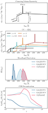 |
Fig. 1. Summary of the modeling in our analysis. We characterized the UV volume emissivity ϵ(ν, z) based on Eqs. (3)–(6) (panel 1). Emissions from different z contribute to the EBL (panel 2, the dots show λrest = 1500 Å; the Lyα line is in absorption at low z), which is weighted by the detector response function in the broadband observation in Eq. (10) (panel 3). The CBR allowed us to reconstruct bJ(z)dJνobs/dz in Eqs. (11) and (13) (panel 4). This figure is inspired by Chiang et al. (2019). |
The signal of interest for our analysis is modeled in the next section. Here, we provide an estimate of the noise variance in the maps. As C19 details, by masking the pixels with flux above the detection limit, resolved sources can be separated from the diffuse light contribution. This separation on the map level helps implement the algorithms required to mitigate the foreground noise. On the other hand, a combined analysis of the two components allows us to study the UV intensity field without selection effects. We thus assumed that a procedure similar to C19 has been performed: resolved sources and diffuse light are initially separated to create the maps and estimate their noises and then summed to perform the analysis.
The noise variance per pixel in the “overall” map was estimated based on the 5σ AB magnitude limit mAB, weighted by the different exposure times during the observations. In the case of GALEX NUV and FUV, C19 indicates mAB ∼ 20.5–23.5, and we adopted the intermediate value mAB = 224. For the ULTRASAT reference map, following Shvartzvald et al. (2024), we instead assumed mAB = 23.5 in order to get a factor of ten sensitivity improvement from GALEX.
The limiting magnitude characterizes the detection level above which sources (with Galactic or extragalactic origin) cannot be resolved. For this reason, we can use it to describe the ground level of the observed intensity inside a region with a comparable size to the point spread function. We converted mAB to flux per pixel via mAB = 8.90 − 2.5log10ℱν, and we rescaled it to flux density inside a certain angular region as  . The pixel surface area was computed as
  , where Lpix is the pixel scale. The value obtained corresponds to sources five times brighter than the noise level; hence, we got the total noise variance per pixel
![Mathematical equation: $$ \begin{aligned} \sigma _N^2 = \left[{f_\nu ^\mathrm{pix}}/{5}\right]^2 . \end{aligned} $$](/articles/aa/full_html/2024/07/aa49364-24/aa49364-24-eq4.gif) (2)
(2)
To reduce the value of  , it is always possible to combine the pixels into groups, which we call “effective pixels”. This reduces their number, and it averages noise fluctuation on the smallest scales. We discuss in Sect. 3.4 that, in the context of the CBR analysis, C19 used effective pixels with
  . We show that ULTRASAT will obtain good results already using Lpix. We note that, so far, we have not accounted for foreground contributions; these are described in Sect. 3.4.
Table 1 collects the main survey specifications we discussed so far, and it compares their estimated  value. The table also reports the value of the observed monopole Jνobs, which we define in Sect. 3.2.
Specs of the broadband surveys used in the analysis.
3. Modeling the signal and noise
The broadband measurements ULTRASAT will realize integrate the radiation emitted over a wide frequency and redshift range. Reconstructing the spectral shape of the signal, as well as its evolution across cosmic time, is of fundamental importance to disentangle cosmological dependencies and astrophysical properties of the emitters. One way this goal can be pursued is via broadband tomography, or the CBR technique (Newman 2008; McQuinn & White 2013; Ménard et al. 2013), namely the cross correlation between one broadband survey (ULTRASAT or GALEX, in our case) and a reference spectroscopic galaxy catalog. Using cross correlations allows us to overcome the presence of Galactic foregrounds, ensuring that the measured signal has an extragalactic origin. The possibility of a chance correlation is further reduced by the fact that foregrounds fluctuate mainly at large scales, while we are interested in cross correlations on small scales. Hence, in our analysis, foregrounds only contribute to the noise budget.
The authors of C19 applied CBR to GALEX data in order to constrain the redshift evolution of the UV-EBL volume emissivity. In their case, a subset of the SDSS catalogs (Blanton et al. 2005); Reid:2015gra was adopted as reference. ULTRASAT, with its improved NUV capability, seems to be the perfect heir for this kind of analysis. Considering its timeline, many state-of-the-art galaxy surveys will be available to perform the cross correlation. As we detail in Sect. 3.4, the best results are obtained for small spectroscopic redshift uncertainties and large galaxy number densities in the range under analysis. For this reason, we decided to rely on the forecasted five-year capability of DESI (Levi et al. 2013; Aghamousa et al. 2016a,b), which is depicted in Adame et al. (2024).
To forecast the constraining power ULTRASAT×DESI will have compared to GALEX×SDSS, we now introduce the quantities required to model the observables. In Sect. 3.1, we follow the formalism from C19 and S21, and we describe the UV-EBL volume emissivity that we aim to constrain. The emissivity is then converted into observed intensity in Sect. 3.2. We then review how CBR can reconstruct its redshift evolution in Sect. 3.3, and we estimate the uncertainty in its measurement in Sect. 3.4. Figure 1 summarizes the logic and modeling of the analysis.
3.1. Ultraviolet volume emissivity
The first ingredient we needed in order to model the signal was the spatially averaged comoving volume UV emissivity, ϵ(ν, z) [erg s−1 Hz−1 Mpc−3]. Similar to C19 and S21, we parameterized its frequency and redshift dependencies using a piecewise function capable of describing the different spectral contributions the EBL receives. This model is in agreement with simulation results based on the study of the radiative transfer of Lyman continuum photons in the IGM (Haardt & Madau 2012).
We distinguished between the non-ionizing continuum at λrest > 1216 Å and between 912 Å < λrest ≤ 1216 Å, the Lyα line at λrest = 1216 Å, and the ionizing continuum at λrest ≤ 912 Å below the Lyman break. Above Lyα, we describe the frequency and redshift evolution of the non-ionizing continuum with respect to a pivot value as
![Mathematical equation: $$ \begin{aligned} \epsilon (\nu ,z) = \epsilon _{1500}\left[\frac{\nu }{\nu _{1500}}\right]^{\alpha _{1500}}, \end{aligned} $$](/articles/aa/full_html/2024/07/aa49364-24/aa49364-24-eq11.gif) (3)
(3)
where ν1500 is the frequency at λrest = 1500 Å.
Between the Lyα line and the Lyman break, we adopted
![Mathematical equation: $$ \begin{aligned} \epsilon (\nu ,z) = \epsilon _{1500}\left[\dfrac{\nu _{1216}}{\nu _{1500}}\right]^{\alpha _{1500}} {\left\{ \begin{array}{ll}&\left[\dfrac{\nu }{\nu _{1216}}\right]^{\alpha _{1100}}\,\, \\&\dfrac{\mathrm{EW}}{\nu _{1216}\delta }\dfrac{\nu ^2}{c} + \left[\dfrac{\nu }{\nu _{1216}}\right]^{\alpha _{1100}}, \end{array}\right.} \end{aligned} $$](/articles/aa/full_html/2024/07/aa49364-24/aa49364-24-eq12.gif) (4)
(4)
where the first line holds for |ν − ν1216|> ν1216δ, with δ = 0.005 and line frequency ν1216 = 2.5 × 10⁶ GHz. Finally, in the ionizing range, we set
![Mathematical equation: $$ \begin{aligned} \epsilon (\nu ,z) = \epsilon _{1500}\left[\frac{\nu _{1216}}{\nu _{1500}}\right]^{\alpha _{1500}}f_{\rm LyC}\left[\frac{\nu _{912}}{\nu _{1216}}\right]^{\alpha _{1100}}\left[\frac{\nu }{\nu _{912}}\right]^{\alpha _{900}}, \end{aligned} $$](/articles/aa/full_html/2024/07/aa49364-24/aa49364-24-eq13.gif) (5)
(5)
where fLyC represents the ionizing photons escape fraction, and it determines the presence of the Lyman break and Lyman forest in the spectra of galaxies and quasars (Meiksin & White 2003; Khaire et al. 2019).
The redshift dependencies of Eqs. (3)–(5) are encapsulated in the normalization and slope parameters of the continuum, namely
 (6)
(6)
as well as in the line equivalent width (EW)5,
![Mathematical equation: $$ \begin{aligned} \begin{aligned}&\mathrm{EW} = C_{\rm Ly\alpha }\log _{10}\left(\frac{1+z}{1+z_{\rm EW 1}}\right) + \mathrm{EW}^{z = z_{\rm EW 1}},\\&C_{\rm Ly\alpha } = \frac{\mathrm{EW}^{z = z_{\rm EW 2}}-\mathrm{EW}^{z = z_{\rm EW 1}}}{\log _{10}[(1+z_{\rm EW 2})/(1+z_{\rm EW 1})]}, \end{aligned} \end{aligned} $$](/articles/aa/full_html/2024/07/aa49364-24/aa49364-24-eq15.gif) (7)
(7)
and in the Lyman continuum escape fraction in the IGM,
![Mathematical equation: $$ \begin{aligned} \begin{aligned}&\log _{10}f_{\rm LyC} = C_{\rm LyC}\log _{10}\left(\frac{1+z}{1+z_{\rm C 1}}\right) + \log _{10}f_{\rm LyC}^{z = z_{\rm C 1}},\\&C_{\rm LyC} = \frac{\log _{10}f_{\rm LyC}^{z = z_{\rm C 2}}-\log _{10}f_{\rm LyC}^{z = z_{\rm C 1}}}{\log _{10}[(1+z_{\rm C 2})/(1+z_{\rm C 1})]}. \end{aligned} \end{aligned} $$](/articles/aa/full_html/2024/07/aa49364-24/aa49364-24-eq16.gif) (8)
(8)
Overall, as Fig. 1 shows in the top panel, the amplitude of the volume emissivity is set by ϵ1500(z), while the characteristics of the Lyα line are determined by EW(z) and the amplitude of the Lyman break by fLyC(z). At each z, the αl(z) parameters (l = 1500, 1100, 900) set the slopes of the frequency dependence in the different regimes.
The upper part of Table 2 collects the parameters through which we parameterized the volume emissivity ϵ(ν, z), together with their fiducial values, which we chose to match the posterior results of C19. As for the  parameters, the analysis in C19 only provides 3σ upper bounds. Therefore, in the following, we set these parameters to the largest values allowed by their results. This was done to show the capability ULTRASAT will have in improving the constraints on such upper limits. In Sect. 4.4, we discuss the implications in the case they are set to smaller values.
Parameters to model the emissivity ϵ(ν, z).
To analyze both the GALEX NUV and FUV filters, C19 set the pivot points of the EW in Eq. (7) to {zEW1 = 0.3, zEW2 = 1} and the ones of the escape fraction in Eq. (8) to {zC1 = 1, zC2 = 2}. In our ULTRASAT analysis, we decided to keep the same pivot points for the escape fraction, while we pivoted the EW at {zEW1 = 1, zEW2 = 2}. The higher redshift was chosen according to the ULTRASAT λobs regime, which collects emissions from the Lyα line at zLyα ∈ [0.9, 1.4] (compare with Table 1) and from the Lyman break at z912 ∈ [1.5, 2.2]. To get a continuous signal, we estimated EWz = 2 from Eq. (7) using the C19 pivot points. Figure 1 shows ϵ(ν, z) at different z.
3.2. Observed intensity
The volume emissivity we modeled describes the UV emission at the source. Broadband observations, however, have to deal with a combination of effects to convert this quantity into the observed, integrated specific intensity Jνobs [Jy/sr].
When HI clumps are present along the line of sight, they partially absorb UV radiation before it can be observed. The effective optical depth τ(z) of this phenomenon was originally estimated in Madau (1995), accounting for a Poisson distribution of the absorbers as a function of their column density and redshift. Absorption is efficient for radiation with λrest either smaller than the ionization wavelength 912 Å or comparable with Lyα and other lines in the Lyman series, which give rise to the Lyman forest (Gunn & Peterson 1965; Steidel & Sargent 1987; Madau 1995). In our analysis, we rely on the improved semi-analytical model in Inoue et al. (2014) described by a piecewise power-law in overall agreement with Madau (1995).
The UV volume emissivity in our computation is hence given by ϵ(ν, z)e−τ(ν), where τ(ν) is the optical depth. By using the radiative transfer function in an expanding Universe, it is possible to convert this quantity into a specific intensity (Gnedin & Ostriker 1997) through
 (9)
(9)
where νobs = ν/(1 + z), c is the speed of light and H(z) the Hubble factor. In a broadband survey, such as ULTRASAT or GALEX, observations are performed over a wide range of frequencies and weighted by the detector response function. Hence, the observed monopole is
 (10)
(10)
where R(νobs) is the quantity in Eq. (1) once the wavelength is converted into frequency. We estimated Jνobs = 237 Jy/sr for ULTRASAT and Jνobs = 264 Jy/sr, 79 Jy/sr for GALEX NUV and FUV, respectively, which are in agreement with the measurements presented in C19.
Our modeling of Jνobs only accounts for extragalactic contributions, while real data include foregrounds. As we discuss in the next section, the CBR technique generally provides an unbiased estimator of the extragalactic radiation field, which overcomes the foreground problem. At this stage, we could thus safely rely on a signal model that only contains extragalactic UV contributions and include the foregrounds only in the noise budget.
3.3. Spectral tagging via clustering-based redshifts
The band-averaged specific intensity in Eq. (10) contains the integrated information about the redshift evolution of the UV volume emissivity. The CBR technique (Newman 2008; McQuinn & White 2013; Ménard et al. 2013) offers a possible way to reconstruct the redshift dependence dJνobs/dz, based on the correlation between the broadband survey and the spectroscopic galaxy catalog used as a reference sample.
On one side, the specific intensities Jνobs measured in the pixels of the broadband map provide a dataset with unknown redshifts and whose spatial fluctuations are determined by the way UV emitters trace the underlying large-scale structure (LSS). On the other side, galaxies in the spectroscopic sample trace the LSS as well, and they can be divided into consecutive slices of well-known redshift. The angular cross correlation between the two datasets can then be exploited to remap Jνobs in terms of the redshift-dependent specific intensity:
 (11)
(11)
The amplitude of the correlation, in fact, will peak for intensity-galaxy pairs that trace the LSS in a common redshift range. As C19 has shown, this quantity can be constructed by using the absolute value of the intensity, namely by including foregrounds and Galactic emissions. Even if this is the case, the cross correlation is capable of isolating the extragalactic contribution.
The measurement obtained with CBR, however, is degenerate with the bias of the sources of the unknown redshift sample, namely the UV emitters. Following C19 and S21, we parameterized such bias as
![Mathematical equation: $$ \begin{aligned} b(\nu ,z) = b_{1500}^{z=0}\left[\frac{\nu }{\nu _{1500}}\right]^{\gamma _{b_\nu }}(1+z)^{\gamma _{b_z}}, \end{aligned} $$](/articles/aa/full_html/2024/07/aa49364-24/aa49364-24-eq32.gif) (12)
(12)
where we normalized the frequency dependence to the value at 1500 Å, analogously to the other parameters used to model the emissivity in Sect. 3.1. Fiducial values are collected in Table 2. The value of  is degenerate with
  in determining the amplitude of the signal, as becomes evident in the following section.
In the data of the UV broadband survey, the information on the clustering enters through an effective intensity-weighted bias bJ(z), which is computed from the source bias in Eq. (12) through
 (13)
(13)
To model the CBR observable, we started by defining the fluctuations in the map measurements in terms of the angular position ϕ as
 (14)
(14)
where ⟨Jνobs⟩ is the ensemble average. The galaxy survey was instead used to trace the 3D overdensity field through
 (15)
(15)
where ng(ϕ, z) is the galaxy number density, bg(z) is the galaxy bias, and δm(ϕ, z) describes the LSS overdensities in the underlying dark matter field.
The choice of the reference galaxy survey depends on the redshift range and precision one wants to achieve. C19 uses SDSS data from Blanton et al. (2005), Reid et al. (2016), but we decided to adopt the forecasts for the five-year results of DESI, described in Adame et al. (2024). As Table 3 shows, both surveys provide catalogs mapping different kinds of sources. Figure 2 shows the number of galaxies they contain in each redshift bin, namely
 (16)
(16)
Specs of the galaxy surveys considered in this work.
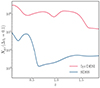 |
Fig. 2. Number of galaxies per redshift bin with size Δz = 0.1. The values for DESI are from Adame et al. (2024), while those for SDSS are from Blanton et al. (2005), Reid et al. (2016). Discontinuities are due to different catalogs. |
where dNg/dzdΩ is the number of galaxies per steradian per redshift bin, Ωsurvey is the sky area observed by the survey, and Δzi the width of the bin.
The angular cross correlation between the intensity pixels and galaxies that are separated by an angle θ on the sky was ultimately defined as
 (17)
(17)
and then marginalized over θ in order to get
 (18)
(18)
This is the main observable we are interested in our analysis. The choice of the window function W(θ) was arbitrary.
In analogy with C19 and S21, we chose W(θ) = θ−0.8/∫θ−0.8dθ. The minimum angular distance above which the cross correlation is performed was set to θmin(z) = arctan[rmin/DA(z)], where DA(z) is the cosmological angular diameter distance and rmin = 0.5 Mpc is a physical scale chosen to avoid strong non-linear clustering on small scales. To provide a more conservative result, in Sect. 4 we also consider the case in which rmin = 1 Mpc−1. For z ∈ [0.1, 2], we got θmin ∈ [4, 0.97] arcmin, larger than Lpix in Table 1. The choice of θmax instead was set to avoid large fluctuations in the calibration of the map. In our case, ULTRASAT has a wide field of view (FoV) ΩFov = 204 deg2, across which observational properties vary. Shvartzvald et al. (2024) shows that the effective point spread function is almost constant up to ∼4 deg from the center of the FoV. Therefore, we assumed that inside this range, calibrations are stable, and we ran our analysis up to θmax = 4 deg. In the case of GALEX, C19 instead chose θmax(z) = arctan[5 Mpc.DA(z)] ∈ [44,10] arcmin = [0.7,0.2] deg. We adopted the same value when dealing with GALEX.
The angular cross correlation  defined in Eq. (18) represents the CBR observable and can be used to infer the redshift evolution of the specific intensity. In fact, we can re-express it as
 (19)
(19)
where bJ(z) and bg(z) are the biases of the two LSS tracers and ωm(θ, z) is the angular two-point function of the underlying dark matter field. This can be related to the non-linear matter power spectrum (Maller et al. 2005) via
 (20)
(20)
where 𝒥0 is the Bessel function of the first type, χ(z) the radial comoving distance, and dz/dχ = H(z)/c. We computed the Pm(k, z) dark matter power spectrum using the public library CAMB6 (Challinor & Lewis 2011), and we adopted the halofit model prescription from Mead et al. (2021).
The observation of  then leads to the reconstruction of the redshift evolution of the intensity weighted by the bias,
  . This in turn represents a summary of the statistics of the UV emission and absorption across space and time. We show
  in Fig. 1 for ULTRASAT and GALEX (NUV, FUV), while Fig. 3 shows the CBR signal-to-noise ratio of
  when their maps are cross correlated with the galaxy reference catalogs from SDSS or DESI. These are the quantities that enter our analysis in Sect. 4.
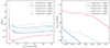 |
Fig. 3. Noise analysis for ULTRASAT×DESI (pink), GALEX NUV×SDSS and ×DESI (light blue, dashed and continuous), and GALEX FUV×SDSS and ×DESI (dark blue, dashed and continuous). Left: 𝒩CBR from Eq. (25). Here, we consider different sizes for the effective pixels. For each detector, the dot indicates the noise for Lpix as in Table 1, while the cross indicates the value adopted in the analysis. Right: S/N obtained from Eqs. (19) and (25). |
3.4. Noise
Newman (2008), Ménard et al. (2013) analytically estimated the uncertainty on the CBR angular cross correlation  introduced in Eq. (19). We followed a reasoning similar to theirs, accounting for the fact that the broadband UV data are measured as intensity in pixels rather than point sources, which is the approach in photometric galaxy surveys7.
In the broadband survey, we modeled the monopole in each pixel by summing the EBL from Eq. (10) with an estimate of the foreground. This provided an offset between the expected and observed Jνobs that has indeed been observed. The authors of Akshaya et al. (2018) estimated the observed surface brightness in photon units8 to be ∼250 ph cm−2s−1sr−1Å−1 in the FUV band and ∼550 ph cm−2s−1sr−1Å−1 in the NUV band. C19 explains the offset as being due to the presence of three main foregrounds: near-Earth airglow and zodiacal light (the latter being relevant only in the NUV band; see Murthy 2013), Galactic dust, and a component whose origin is unknown. We accounted for all of these sources by adding to the EBL monopole a fractional contribution 𝒜fgJνobs so that  . We set 𝒜fg = 1.8 for GALEX FUV and 2.2 for GALEX NUV and ULTRASAT since they observe similar bands. We assumed data are Poisson distributed over pixels (thus we estimated the variance as the signal mean value), while fluctuations are Gaussian, with variance
  from Eq. (2). Hence, the total noise is
![Mathematical equation: $$ \begin{aligned} \sigma _J^2 = [J_{\nu _{\rm obs}}(1+\mathcal{A} _{\rm fg})]^2 +\sigma _N^2. \end{aligned} $$](/articles/aa/full_html/2024/07/aa49364-24/aa49364-24-eq51.gif) (21)
(21)
As described in Sect. 3.3, the CBR cross correlation was computed in patches of area  , where θmax = 4 deg for ULTRASAT and θmax ∼ [0.7, 0.2] deg for GALEX. Therefore, to infer the noise, we needed to account for all the possible pairs of pixels and reference galaxies per redshift bin that can be created inside the patches. We rescaled the total number of pixels
  inside
  as
as
 (22)
(22)
where we used  , Ωsky being the sky area observed by the broadband survey, while
  is the area of the pixels computed using Table 1. Meanwhile, the number of galaxies per z bin in the same area is
 (23)
(23)
where Ng, i = ΔziΩsurveydNg/dzdΩ is the number of reference galaxies in the observed area of the survey Ωsurvey in the ith redshift bin having size Δzi (see Fig. 2).
Finally, we estimated the number of pairs to be
![Mathematical equation: $$ \begin{aligned} N_{\rm pairs} = N_{\rm pix}N_{g,i}^{\theta _{\rm max}} = \frac{N_{g,i}}{A_{\rm pix}}\frac{(\pi \theta _{\rm max}^2)^2}{\mathrm{min}[\Omega _{\rm survey},\Omega _{\rm sky}]}. \end{aligned} $$](/articles/aa/full_html/2024/07/aa49364-24/aa49364-24-eq59.gif) (24)
(24)
In the case of ULTRASAT×DESI and GALEX×DESI, the observed area is set by the galaxy survey, namely Ωsurvey = 14 000 deg2 (Adame et al. 2024). Following the procedure in C19, instead, for GALEX×SDSS we set Ωsurvey = 5500 deg2, which is the size of the overlapping footprints. Analogous to S21 and Chiang & Ménard (2019), for SDSS we set Δzi = 0.1; hence we sampled the [0, 2] redshift range with 20 bins. This width is larger than the uncertainty of the spectroscopic redshift bins δzi. In fact, as has been shown in Ménard et al. (2013), Rahman et al. (2015), CBR provides a measurement of the redshift that is degenerate with the bias evolution in z. This degrades the goodness of the redshift inferred using CBR, and it can lead to the overlap between contiguous bins when their width is too small. Moreover, using redshift bins that are too small would increase the shot noise term encapsulated in Ng, i. In the case of SDSS, the width Δzi = 0.1 allowed us to overcome this issue. In the case of DESI, we made the conservative choice of using the same redshift bin width.
Moreover, a further contribution to the CBR noise comes from the width δzi of the spectroscopic bins. Assuming that matter clusters on scale δzc and not beyond, a galaxy survey with either bins δzi ≫ δzc or δzi < δzc would not be precise in reconstructing the dJνobs/dz redshift evolution based on cross correlation information. The best strategy according to Ménard et al. (2013) is to choose reference redshift bins with δzi ∼ δzc ∼ 10−3; in this way, the amplitude of the cross correlation between the intensity and a reference galaxy is high only locally, that is, inside the redshift bin from where the intensity comes from. Following Ménard et al. (2013), we accounted for this type of noise through a δzi/δzc factor, where we set δzc = max[10−3, H(z)(1 + z)rmin] to avoid strong non-linear clustering and accounted for redshift evolution in the clustering scale. The quantity rmin is the same minimum physical distance adopted in Sect. 3.3 to define the size of the patches in which the cross correlation is computed. On the other hand, we defined the width of the spectroscopic bins δzi for SDSS and DESI as the largest value between δzc and the instrumental resolution λ/Δλ in Table 3.
Finally, we needed to account for the number of sky patches Nθ, over which the statistical analysis can be performed. This introduces an extra  factor. Collecting all the elements described up to this point, we estimated the noise in the CBR procedure to be
![Mathematical equation: $$ \begin{aligned} \mathcal{N} _{\rm CBR}&= \frac{\delta z_i}{\delta z_c}\sqrt{\frac{\sigma _J^2}{N_{\rm pairs}N_{\theta }}} \nonumber \\&= \frac{\delta z_i}{\delta z_c}\sqrt{\frac{A_{\rm pix}{\bigl [[J_{\nu _{\rm obs}}(1+\mathcal{A} _{\rm fg})]^2 + \sigma _N^2\bigr ]}}{\pi \theta _{\rm max}^2N_{g,i}}}. \end{aligned} $$](/articles/aa/full_html/2024/07/aa49364-24/aa49364-24-eq61.gif) (25)
(25)
The CBR noise 𝒩CBR clearly depends on the properties of both the broadband and galaxy surveys. To minimize it, on one side we need a spectroscopic survey where the uncertainty δzi is small but that observes enough galaxies to guarantee a high Ng, i. The former condition enables us to improve the quality of the clustering redshift estimation, while the latter reduces the shot noise. On the other side, a sweet spot exists between using small pixels and getting a not-too-large value for  ; in fact, using smaller pixels would provide a larger number of pairs, hence a smaller statistical noise. The flux density per pixel
  defined in Sect. 2, however, increases when the area of the pixels gets smaller, leading to a larger
  . On the other hand, the uncertainty due to the statistical Poissonian fluctuations encapsulated in Jνobs(1 + 𝒜fg) determines a ground level for the error budget. Since the noise variance cannot be lower than the monopole expected in the map from the astrophysical contribution, the optimal value is reached when
 ![Mathematical equation: $ \sigma_N^2 \sim [J_{\nu_{\rm obs}}(1+\mathcal{A}_{\rm fg})]^2 $](/articles/aa/full_html/2024/07/aa49364-24/aa49364-24-eq65.gif) . By looking at Table 1, it is evident that ULTRASAT already satisfies this condition with Lpix, while GALEX requires the use of larger effective pixels. As Fig. 3 shows, this translates to two different prescriptions when computing 𝒩CBR. While for ULTRASAT the pixel scale Lpix is already good enough to minimize the noise, for GALEX it is better to group the pixels in order to reach an effective scale
. By looking at Table 1, it is evident that ULTRASAT already satisfies this condition with Lpix, while GALEX requires the use of larger effective pixels. As Fig. 3 shows, this translates to two different prescriptions when computing 𝒩CBR. While for ULTRASAT the pixel scale Lpix is already good enough to minimize the noise, for GALEX it is better to group the pixels in order to reach an effective scale  , which is indeed the one adopted in C19. In this case, the noise variance is
  . Finally, the difference between NUV and FUV is due to the different Jνobs. Accurate foreground cleaning and mitigation can reduce the noise with respect to the value we estimated.
Under this choice of parameters, we estimated the noise 𝒩CBR to be used in the analysis shown in Sect. 4. Figure 3 compares the signal-to-noise ratio  estimated for all the surveys. The redshift dependence is evident in the signal, while in the noise, it only enters in the choice of θmax for GALEX and the estimate of δzi/δzc. By looking at GALEX in this plot, it is clear that the cross correlation with DESI will lead to a larger S/N: this is due both to the better spectroscopic redshift determination and to the larger number of galaxies observed. The comparison between GALEX NUV×DESI and ULTRASAT×DESI in this figure reflects the smaller noise ULTRASAT has thanks to its smaller Apix and wider θmax.
4. Forecasts
To constrain the parameters of the UV-EBL emissivity, C19 analyzes data from GALEX×SDSS. Since our final goal is to perform a forecast analysis, we relied instead on the Fisher matrix formalism (Vogeley & Szalay 1996; Tegmark et al. 1997). For each detector-galaxy survey pair, we computed the Fisher matrix by summing over the i-redshift bins of the CBR analysis as
 (26)
(26)
where the noise 𝒩CBR(zi) is estimated in Eq. (25).
The parameter set is
![Mathematical equation: $$ \begin{aligned} \begin{aligned} \vartheta =&\{\log _{10}[b\epsilon ]_{1500}^{z=0},\,\gamma _{1500}, \,\gamma _{\nu },\,\gamma _z\\&\alpha _{1500}^{z=0},\,C_{1500},\,\alpha _{1100}^{z=0},\,C_{1100},\,\alpha _{900}^{z=0},\\&\mathrm{EW}^{z=z_{\rm EW1}},\,\mathrm{EW}^{z=z_{\rm EW2}},\\&\log _{10}f_{\rm LyC}^{z=z_{\rm C1}},\,\log _{10}f_{\rm LyC}^{z=z_{\rm C2}}\}, \end{aligned} \end{aligned} $$](/articles/aa/full_html/2024/07/aa49364-24/aa49364-24-eq70.gif) (27)
(27)
which collects the parameters introduced in Table 2. Whenever we wanted to account for priors on certain parameters, we summed the Fisher matrix with the prior matrix, which has  diagonal elements. The marginalized error on each ϑα can ultimately be estimated from the inverse of the Fisher matrix (already summed with the prior matrix, if needed) as
  . The forecasts can then be propagated to estimate the uncertainty on the volume emissivity ϵ(ν, z) or on the ionizing photon escape fraction fLyC using
  , where ℵ is the new parameter, 𝒟ℵ, ϑ = (∂ℵ/∂ϑα,...) is the vector of its derivatives with respect to the old ones, and F is the Fisher matrix in Eq. (26).
Before proceeding, it is important to remember that, while being extremely useful for order-of-magnitude estimates, the Fisher matrix formalism usually provides optimistic forecasts. In particular, the marginalized errors it obtains tend to underestimate the uncertainty in the presence of significant degeneracies between the parameters. (For a comparison between forecasts obtained using a Markov chain Monte Carlo approach and the Fisher approach, see, for example, Wolz et al. 2012, and references within.)
4.1. Breaking the bias degeneracy
As discussed in Sect. 3.2, the normalization value  and the local bias
  are degenerate. For this reason, in our analysis, we collected them in a single parameter
 ![Mathematical equation: $ \log_{10}[\epsilon b]_{1500}^{z=0} $](/articles/aa/full_html/2024/07/aa49364-24/aa49364-24-eq76.gif) . Moreover, results in C19 and S21 show further degeneracies between the parameters that determine the slope of the bias, namely {γbν, γbz}, and the ones that characterize how the emissivity depends on the frequency and redshift.
. Moreover, results in C19 and S21 show further degeneracies between the parameters that determine the slope of the bias, namely {γbν, γbz}, and the ones that characterize how the emissivity depends on the frequency and redshift.
To overcome these issues, we introduced Gaussian priors on {γbν, γbz}; in particular, we relied on C19 results and set σγbν = 1.30, σγbz = 0.30. These are indeed the largest errorbars C19 obtained from the GALEX×SDSS CBR analysis and can thus be interpreted as a conservative choice for our forecasts. To these priors, we added the ones C19 uses on {γ1500, C1500, C1100}. Imposing a prior σ = 1.3 on γ1500 and wide Gaussian priors with σ = 1.5 on C1500, C1100 is still needed in the case of GALEX×SDSS, while they can be removed when using DESI.
The motivation behind our prior choice relies on the fact that our main targets are the parameters regulating the emissivity, while the bias can potentially be constrained from different probes, such as the resolved sources catalog of the broadband survey itself. In C19, such a possibility is explored by estimating the bias of the GALEX resolved sources and rescaling its value to the EBL regime. To do so, they assumed that the bias of the resolved sources is larger than the bias of the EBL diffuse light map due to the flux-limit that allows us to resolve only of the brightest, and thus more clustered, sources. The analysis was done accounting for the information on the GALEX redshift-dependent luminosity threshold and the luminosity-dependent SDSS galaxy bias in Zehavi et al. (2011), and it returned an estimated errorbar  .
.
We assumed that a similar procedure will be applied to ULTRASAT×DESI and GALEX×DESI. The estimated errorbars in those cases will reasonably be ≤0.05. Similar to what C19 discusses, this will make it possible to break the degeneracy between  and
and  . Hence, in the following, we present results for ϵ(ν, z). These were obtained by marginalizing over
  with Gaussian priors respectively {0.05, 0.30, 1.30}. We stress again that these values were chosen according to GALEX×SDSS results and therefore represent a conservative choice in our forecast. To get a more optimistic result, we also tested the case {0.01, 0.10, 0.30}. The priors are summarized in Table 4.
Priors on the bias parameters.
4.2. Validation and parameter forecast
To validate our results, we first applied the Fisher formalism to GALEX FUV×SDSS and NUV×SDSS, and we tried to “post-dict” the results in C19. We used the same reduced parameter set that they adopted, namely
![Mathematical equation: $$ \begin{aligned}&\vartheta _{\rm C19}=\left\{ \log _{10}[\epsilon b]_{1500}^{z=0},\,\gamma _{1500},\alpha _{1500}^{z=0},\,C_{1500},\,\alpha _{1100}^{z=0},\right.\nonumber \\&\qquad \qquad \left. C_{1100},\,\mathrm{EW}^{z=0.3},\mathrm{EW}^{z=1},\,\gamma _{\nu },\,\gamma _z\right\} . \end{aligned} $$](/articles/aa/full_html/2024/07/aa49364-24/aa49364-24-eq82.gif) (28)
(28)
Here, we fixed all the parameters related with the ionizing continuum below the Lyman break in Eq. (5), for which C19 showed that GALEX×SDSS has no constraining power, and we adopted the priors in Table 4.
We ran the analysis in Eq. (26) separately for the NUV and FUV filters, and we assumed that they are uncorrelated so that we could sum their matrices in order to improve the constraints. The fact that the filters are sensitive to different ranges is crucial to capturing the shape of the redshift-dependent parameters in Eq. (6) and better reconstructing ϵ(ν, z). A further confirmation of this can be seen in the good results the authors of S21 obtained when combining the three CASTOR filters.
Our results are collected in Table 5 and were compared with the actual results of C19. Notably, our Fisher forecasts are in the same ballpark. However, our analysis lacks the ability to accurately reproduce constraints on the EW parameters. The reason for this resides in the fact that these parameters only affect a small portion of the spectrum described in Eq. (4); hence, they introduce a discontinuity in the analytical model that is more difficult to capture in the computation of the numerical derivatives required in Eq. (26)9. Despite this, the EW parameters are not degenerate with the others, and thus they do not alter the result on the other marginalized errors estimated from the Fisher matrix computation.
One-sigma marginalized errors from our “post-diction” for GALEX×SDSS.
Since our “post-diction” is reasonable, we proceeded by applying it to the ULTRASAT×DESI scenario. As we discuss in Sect. 3.1, in this case we decided to pivot the evolution of the EW at higher redshift, namely zEW1 = 1, zEW2 = 2. Table 5 presents the results we found. The constraining power increased with respect to GALEX×SDSS on all the parameters except ![Mathematical equation: $ \log_{10}[\epsilon b]_{1500}^{z=0} $](/articles/aa/full_html/2024/07/aa49364-24/aa49364-24-eq94.gif) , for which GALEX is helped by the wider redshift range probed by its two filters, NUV and FUV. The ULTRASAT sensitivity at z ∼ 1 leads to a large improvement in the parameters determining the redshift evolution as well as in the line EW. In the case of ULTRASAT×DESI, there is no need to use priors on {γ1500, C1500, C1100}. We checked that both GALEX×SDSS and ULTRASAT×DESI have no constraining power on the parameters
, for which GALEX is helped by the wider redshift range probed by its two filters, NUV and FUV. The ULTRASAT sensitivity at z ∼ 1 leads to a large improvement in the parameters determining the redshift evolution as well as in the line EW. In the case of ULTRASAT×DESI, there is no need to use priors on {γ1500, C1500, C1100}. We checked that both GALEX×SDSS and ULTRASAT×DESI have no constraining power on the parameters  of the ionizing continuum. Moreover, including them in ϑ worsens the results on the other parameters.
Having shown that ULTRASAT×DESI will improve the constraints, we turned our attention to the full parameter set (GALEX+ULTRASAT)×DESI, which we consider as our baseline in the following sections. In this case, the full set ϑ in Eq. (27) can be tested. As Table 6 shows, all the parameters are indeed well constrained. The only degeneracy not yet solved is the one between γ1500 and γbz, but using a prior on one of them helps constrain the other. Results were obtained by separately computing the Fisher matrices for GALEX NUV×DESI, GALEX FUV×DESI, and ULTRASAT×DESI, then summing them. The full matrix includes the EW pivot parameters at zEW = {0.3, 1, 2}, with zEW = 1 constrained by both of the detectors, while the others were constrained either by GALEX or ULTRASAT.
Forecasted 1σ marginalized errors from our Fisher analysis for (GALEX+ULTRASAT)×DESI.
Our results depend on the choice of rmin = 0.5 Mpc, which we introduced in Sect. 3.3 to avoid strong non-linear clustering. To test the stability of our conclusions with respect to this parameter, we re-ran the Fisher analysis, cutting the angular correlation at scales associated with rmin = 1 Mpc. In this case, the forecasts in Table 6 deteriorate, and the marginalized errors almost double. Despite this, the constraining power remains good even when less optimistic prescriptions are considered. In the next sections, we therefore rely on the constraints obtained in Table 6; other scenarios can be recovered straightforwardly.
4.3. Forecasts on the volume emissivity
The parameters constrained in the previous section were combined in Eqs. (3)–(5) in order to model the UV-EBL volume emissivity. As discussed in Sect. 4.1, we can assume the local bias  is measured and therefore convert the
 ![Mathematical equation: $ \log_{10}[\epsilon b]_{1500}^{z=0} $](/articles/aa/full_html/2024/07/aa49364-24/aa49364-24-eq102.gif) constraints to
constraints to  and consequently ϵ(ν, z) after marginalizing all the other parameters. We analyzed the results on ϵ(ν, z) using this procedure and applying both the conservative and optimistic bias priors in Table 4.
Figure 4 shows our 1σ forecast constraints on ϵ(ν, z) for (GALEX+ULTRASAT)×DESI, at z = {0, 0.5, 1, 2} using the ϑ parameter set. Here, we also show how the GALEX×SDSS results from the previous section propagate to ϵ(ν, z). Our 1σ forecasts in this case were obtained using the reduced ϑC19 and including priors from Table 4, and they can be directly compared with Fig. 6 in C19.
 |
Fig. 4. Forecasts at 1σ on the UV-EBL emissivity ϵ(ν, z) at different redshifts for (GALEX+ULTRASAT)×DESI compared with our “post-diction” at 1σ for GALEX×SDSS as in Chiang et al. (2019) (compare with Fig. 6 in their work). We tested both the optimistic and conservative bias priors described in Table 4. The gray shaded area delimits the observational window of GALEX+ULTRASAT, and the gray vertical line shows where GALEX NUV would stop if ULTRASAT was not included. The parts of the spectrum inside the observed window were directly probed via the CBR, while the others are model-based extrapolations. |
It is evident that (GALEX+ULTRASAT)×DESI will provide very good constraints on the UV-EBL volume emissivity reconstruction. Results could be further improved with respect to our findings if foreground mitigation is taken into account. For example, setting 𝒜fg = 0 in Eq. (21) leads to constraints on the emissivity parameters that are ∼0.5 of the ones in Table 6. Figure 4 allows us to further comment on an important aspect of our analysis: Not all the redshifted wavelengths of the UV-EBL emissivity fall in the observational windows of GALEX+ULTRASAT. The forecast constraints on ϵ(ν, z) that are found in the shaded areas were extrapolated knowing the dependencies of the model parameters in Eqs. (3)–(5). The way these parameters have been chosen is agnostic regarding the physics or the type of sources involved. They only require the UV emission to contain a line (Lyα), a break (the Lyman break), and a continuum whose slope varies in the different frequency ranges. In the following section, we discuss the implications this will have on our knowledge of the UV-EBL sources.
4.4. Forecasts on the UV-EBL sources
The shape of the continuum in the non-ionizing region is shown in C19 to be in good agreement with the model in Haardt & Madau (2012), which accounts for galaxy emission and dust extinction. Haardt & Madau (2012) stresses that the non-ionizing continuum, for instance at 1500 Å, provides valuable information on the star-formation rate history (modeled, e.g., in Madau 1995) and the metal-enrichment history (e.g., in Nagamine et al. 2001; Kewley & Kobulnicky 2007) to be tested against the UV luminosity functions (e.g., Wyder et al. 2005; Reddy & Steidel 2009; Bouwens 2011). Extra-contributions from AGN are negligible in this frequency range, according to Faucher-Giguère (2020). On the contrary, the ionizing continuum λrest < 912 Å seems to be AGN-dominated at z ≲ 4. The result, however, depends on the AGN luminosity function (e.g., Hopkins et al. 2007; Kulkarni et al. 2019; Shen et al. 2020) and on the EBL ionizing photon escape fraction fLyC, with this being largely uncertain. C19 manages to provide only upper bounds on  . In our analysis, we adopted these as our fiducials; however, actual values of fLyC may be smaller than this limit (Flury et al. 2022). We tested how the observable and the forecasts in our analysis change when fLyC is lowered. Since this parameter sets the Lyman break depth (compare with Fig. 1), it mainly determines the shape of dJνobs/dz at high-z, where the signal drops. Therefore, lowering its value only affects the forecasts on
  and on α900. When the escape fraction becomes too small, CBR can no longer constrain the EBL at small wavelengths.
As a final remark, we refer to Fig. 5 to show that (GALEX+ULTRASAT)×DESI will be able to determine the amplitude and redshift evolution of the non-ionizing continuum at λ = 1500 Å up to z ∼ 2, with 1σ uncertainty ≲26% (9%) and with conservative (optimistic) bias priors (see Table 4). We compared our forecasts with the constraints Schiminovich et al. (2005) obtained using the galaxy UV luminosity function in GALEX and with the ones Dahlen et al. (2006), Reddy et al. (2008) obtained from data compilations from the Hubble Space Telescope. Moreover, we included the fitting Dominguez et al. (2011) realized over multiband Spitzer data and the semi-analytical models of Gilmore et al. (2012), which account for different dust models10.
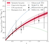 |
Fig. 5. 1σ forecasts on the non-ionizing λ = 1500 Å continuum for (GALEX+ULTRASAT)×DESI (shaded area), with conservative and optimistic priors on the bias. To get GALEX×SDSS (C19) results, we propagated our “post-diction” in Sect. 4.2. We compare with available results in the literature. Schiminovich et al. (2005) data are based on the UV luminosity function of the galaxies in GALEX, Dahlen et al. (2006) on the GOODS survey from the Hubble Space Telescope, while Reddy et al. (2008) use a compilation of data from Hubble. The green line reproduces the fitting of Dominguez et al. (2011) over multiband data, while the dotted lines are the semi-analytical models obtained in Gilmore et al. (2012) with different dust prescriptions. |
The improved forecast constraints we obtained on the ϑ parameters can be used to constrain the astrophysical sources of the UV-EBL. With such measurements, the combination of GALEX and ULTRASAT maps will open the possibility of disentangling any extra contribution due to emissions beyond galaxies and AGN (e.g., from decaying dark matter). We will analyze this enticing possibility in an upcoming, dedicated work.
5. Conclusion
Many satellites are planned to be launched and start operating in the coming years. Their characteristics and goals are very diverse, and it is crucial to understand how to exploit their data as best as we can. New observables and estimators will be needed in order to probe the Universe at various redshifts and scales so as to deepen our understanding of cosmic evolution.
Among these space-borne observatories, ULTRASAT Sagiv et al. (2014), Ben-Ami et al. (2022), Shvartzvald et al. (2024) will observe the NUV range between 2300 Å and 2900 Å, and its main goal will be the study of transients, such as supernovae, variable stars, AGN, and electromagnetic counterparts to gravitational-wave sources. To perform its intended analysis, ULTRASAT will first build a reference full-sky map, which itself will contain an enormous amount of information. In addition, during the lifetime of the mission, its LCS will provide an even deeper map, with a sensitivity approximately ten times better than the full-sky one, and covering an area of ∼6800 deg2.
Besides emission from resolved galaxies, the map will collect diffuse light of astrophysical and cosmological origin, produced for example by unresolved galaxies, AGN, and dust (Madau & Dickinson 2014; Bernstein et al. 2002; Haardt & Madau 2012) or more exotic components such as decaying or annihilating dark matter or direct-collapse black holes (Dwek et al. 1998; Bond et al. 1986; Yue et al. 2013; Creque-Sarbinowski & Kamionkowski 2018; Kalashev et al. 2019; Bernal et al. 2021; Carenza et al. 2023). Notably, the overlap of all of these processes produces the EBL, which in the UV regime is not yet well constrained.
The ULTRASAT full-sky map will be a good tool to boost our knowledge in this field. One method to find different ways to exploit its potential is to look at the studies thatFor revised versions, the pdf with marked changes (bold or diff) should also be uploaded (in optional files). were performed on the full-sky map realized with the All-Sky and Medium Imaging Surveys performed by GALEX Martin et al. (2005), Morrissey et al. (2007). Similarly to GALEX, ULTRASAT will observe a broad frequency range; hence, it will collect the integrated UV emission over a wide redshift range and map its intensity fluctuations as a function of sky position.
The GALEX diffuse light map has been analyzed by the authors of Chiang et al. (2019) (C19) via the CBR technique (Newman 2008; McQuinn & White 2013; Ménard et al. 2013). By cross correlating it with the spectroscopic galaxy catalogs from SDSS Blanton et al. (2005), Reid et al. (2016), they reconstructed the redshift evolution of the comoving volume emissivity of the UV-EBL, providing constraints on the parameters that describe the non-ionizing continuum and the Lyα line. Significantly, these parameters can in turn be used to constrain properties such as the star-formation rate or metallicity history.
A very interesting aspect of CBR is that it is only sensitive to extragalactic contributions, and therefore the presence of foregrounds does not alter its signal but contributes to the overall noise budget. Inspired by the work in (C19), Scott et al. (2022) (S21) developed a forecast analysis to determine the constraining power of CASTOR (Cote et al. 2019). CASTOR has been proposed to have three filters, collecting radiation from λobs ∼ 1500 Å to λobs ∼ 5500 Å. This will make the analysis sensitive to the EBL in the optical region as well as to the UV-EBL sourced at a higher redshift. The use of three filters will further boost the capability of breaking the internal degeneracies between the parameters in the CBR analysis, leading to a better understanding of the EBL cosmic evolution. Further improvements may also come from future experiments that will improve the sensitivity in the FUV band already covered by GALEX. An interesting possibility in this case will be offered by the Ultraviolet Explorer (Kulkarni et al. 2021).
In this work, we studied how to build forecasts for the CBR technique when applied to the cross correlation between a broadband UV survey and a spectroscopic galaxy catalog. We summarized how to model the main observable that is required in this context, namely the angular cross correlation between intensity measurements in pixels and galaxies, and we derived an analytical expression to estimate its noise. We then ran a Fisher forecast with respect to the parameters that model the UV-EBL comoving volume emissivity.
To validate our method, we first reproduced the setup of the analysis performed in C19, where GALEX×SDSS is considered. The constraints we obtained are comparable with the actual results. Once we tested the reliability of our analysis, we applied it to forecast the cross correlation between ULTRASAT full-sky maps and galaxies in the spectroscopic bins of DESI (Levi et al. 2013; Aghamousa et al. 2016a,b). We verified that the smaller redshift uncertainty and larger galaxy number density that DESI has with respect to SDSS, together with the smaller noise variance and larger FoV in the ULTRASAT map, will imply an improvement in the ULTRASAT×DESI constraints with respect to GALEX×SDSS when applied to the same parameter set and under the same conditions.
While in the main text we relied on the ULTRASAT full-sky map, we also analyzed the case of the LCS. Its approximately ten-times better magnitude limit (24.5 vs. 23.5) and around one-half smaller FoV (14 000 deg2 vs. 6800 deg2) lead to forecasts that are ∼10% worse than the ones described in Table 6. We note, however, that the specifics we assumed for the full-sky map are optimistic since we did not model in detail the calibration and foreground cleaning procedures. Meanwhile, the 24.5 magnitude cut for the LCS represents a conservative choice. Therefore, the constraints that will be obtained from it will be comparable with our forecasts in Table 6.
Driven by this result, we applied the forecasted CBR analysis also to the (GALEX+ULTRASAT)×DESI full setup. We showed that the large redshift range and the improved sensitivity will allow us to constrain, with good accuracy, all the parameters in the emissivity model. Once propagated to the emissivity uncertainty, these will lead to the forecasts shown in Fig. 4, where we accounted for different choices of priors on the bias parameters.
Our results implicitly account for an approximation, namely the uncorrelation between datasets, that allows us to simply sum the Fisher matrices in Eq. (26). Accounting for the correlation between the different datasets is not straightforward. The correlation may arise either because we used the same spectroscopic catalog as the reference for the CBR or because the UV-EBL observed by GALEX FUV, GALEX NUV, and ULTRASAT have common sources. To estimate how much this would affect our considerations, we considered an extreme scenario: We separated the reference galaxy catalog into three groups, and each was cross correlated with only one diffuse light map. Further, we masked in each full-sky map two-thirds of the voxels in order to avoid double counting the same sources among the different maps. This led to around a factor of two worse constraints with respect to Table 6.
To further explore this point, we removed from the analysis the Fisher matrix associated with GALEX NUV. Since the FUV filter and ULTRASAT observe non-overlapping bands (see Fig. 1), sources that are relevant for the UV-EBL in one of them may not necessarily be relevant for the other. Moreover, using the ULTRASAT map realized in the LCS map would require only half of the DESI catalog. We could hence cross correlate GALEX FUV with the other half of its footprint. This drastically reduces the correlation between the datasets, and it allowed us to safely use F = FFUV + FLCS. The results are ≲50% worse than the values collected in Table 6, but even in this case, our technique leads to a good improvement with respect to current constraints on the UV-EBL.
We found that (GALEX+ULTRASAT)×DESI will be able to constrain the full UV emissivity frequency dependence in the redshift range z ≲ 2. In our work, we assumed that the total emissivity is composed of different contributions: the non-ionizing continuum, the Lyα line, and the ionizing continuum above the Lyman break. The amplitude and slope of each of these elements is determined by the UV-EBL sources. Therefore, this measurement will provide interesting insights into the galaxy astrophysics. In Fig. 5, we show our forecasts on the non-ionizing EBL emissivity at λ = 1500 Å. In the figure, the current data show an overall agreement with the EBL models that accounts for galaxies, AGN emissions, and dust. The improvement (GALEX+ULTRASAT)×DESI will foster our understanding of this regime, opening a window to the detection of exotic cosmological emissions, if there are any.
To conclude, we stress once again how the study of the UV-EBL will be crucial in the upcoming years. ULTRASAT, with its reference map, will offer the possibility of mapping its intensity fluctuations across the full sky, offering a tool to probe the underlying LSS in a novel, alternative way. To be able to exploit the enormous amount of scientific information this UV full-sky map will contain, developing specific tools for its analysis is important, and the cross correlation with galaxy surveys, in particular in the context of the CBR analysis, is indeed one such tool.
The map will use an integration time of 15 000 seconds at Galactic latitudes |b|> 30 deg. See the ULTRASAT official website for more details: https://www.weizmann.ac.il/ultrasat/.
In the LCS, ULTRASAT is planned to observe 40 extragalactic fields, with 900s of integration time each, over the full duration of the mission. This will result in a theoretical limiting magnitude of ∼24.5–25.5.
GALEX response functions are provided in the public repository http://svo2.cab.inta-csic.es/svo/theory/fps3/
The value is chosen consistently with analysis in C19. We thank Y. K. Chiang for discussion.
The EW is usually defined as the side of a rectangle whose height is equal to the continuum emission, and the area is the same as the line itself, namely EW = ∫dλ(1 − Js(λ)/Jc(λ)), where Jc(λ) is the continuum intensity, while Js(λ) = Jl(λ)+Jc(λ) is the spectrum intensity, including both the continuum and the line. In our convention, a positive value of EW gives rise to an emission line, while a negative value produces an absorption line.
S21 computed the noise differently. In particular, their forecast analysis is built directly on  instead of
  , and thus their noise estimate refers to this quantity.
In photon units, the EBL monopole is 89 ph cm−2s−1sr−1Å−1 for FUV and 172 ph cm−2s−1sr−1Å−1 for NUV.
See also the discussion on the practicality of the Fisher matrix compared to Markov chain Monte Carlo analysis in Wolz et al. (2012).
We followed the notation in C19, where ϵ(ν, z) is the comoving specific emissivity. This is different from Haardt & Madau (2012), where this symbol indicates the proper volume emissivity. Here, ϵ1500(z) coincides with the luminosity density, while in Haardt & Madau (2012), Schiminovich et al. (2005), the luminosity density is indicated with ρ1500.
Acknowledgments
The authors thank Yi-Kuan Chiang for his comments, which helped improving the quality of the paper. A special thanks goes to José L. Bernal for his insights and suggestions about the analysis, and to the anonymous referee for their comments. We thank the ULTRASAT Collaboration for useful discussion about the project, and Brice Ménard, Yossi Shvartzvald and Marek Kowalski for feedback on the manuscript. SL thanks the Azrieli Foundation for support and the Padova Cosmology group for hospitality during the tough times between October 7th and November 2023. SL is supported by an Azrieli International Postdoctoral Fellowship. EDK was supported by a Faculty Fellowship from the Azrieli Foundation. EDK also acknowledges joint support from the U.S.-Israel Bi-national Science Foundation (BSF, grant No. 2022743) and the U.S. National Science Foundation (NSF, grant No. 2307354), and support from the ISF-NSFC joint research program (grant No. 3156/23).
References
- Adame, A. G., Aguilar, J., Ahlen, S., et al. 2024, AJ, 167, 62 [NASA ADS] [CrossRef] [Google Scholar]
- Aghamousa, A., Aguilar, J., Ahlen, S., et al. 2016a, arXiv e-prints [arXiv:1611.00036] [Google Scholar]
- Aghamousa, A., Aguilar, J., Ahlen, S., et al. 2016b, arXiv e-prints [arXiv:1611.00037] [Google Scholar]
- Akshaya, M. S., Murthy, J., Ravichandran, S., Henry, R. C., & Overduin, J. 2018, ApJ, 858, 1538 [Google Scholar]
- Asif, A., Barschke, M. F., Bastian-Querner, B., et al. 2021, Proc. SPIE, 11821, 118210U [NASA ADS] [Google Scholar]
- Bastian-Querner, B., Kaipachery, N., Küster, D., et al. 2021, Proc. SPIE, 11819, 118190F [NASA ADS] [Google Scholar]
- Bates, D. J., Tojeiro, R., Newman, J. A., et al. 2019, MNRAS, 486, 3059 [CrossRef] [Google Scholar]
- Ben-Ami, S., Shvartzvald, Y., Waxman, E., et al. 2022, Proc. SPIE, 12181, 1218105 [NASA ADS] [Google Scholar]
- Bernal, J. L., & Kovetz, E. D. 2022, A&A Rev., 30, 5 [NASA ADS] [CrossRef] [Google Scholar]
- Bernal, J. L., Caputo, A., & Kamionkowski, M. 2021, Phys. Rev. D, 103, 063523 [Erratum: Phys. Rev. D 105, 089901 (2022)] [NASA ADS] [CrossRef] [Google Scholar]
- Bernstein, R. A., Freedman, W. L., & Madore, B. F. 2002, ApJ, 571, 107 [NASA ADS] [CrossRef] [Google Scholar]
- Blanton, M. R., Schlege, D. J., Strauss, M. A., et al. 2005, AJ, 129, 2562 [NASA ADS] [CrossRef] [Google Scholar]
- Bond, J. R., Carr, B. J., & Hogan, C. J. 1986, ApJ, 306, 428 [NASA ADS] [CrossRef] [Google Scholar]
- Bouwens, R. J., et al. 2011, ApJ, 737, 90 [NASA ADS] [CrossRef] [Google Scholar]
- Brown, T. M., Kimble, R. A., Ferguson, H. C., et al. 2000, AJ, 120, 1153 [NASA ADS] [CrossRef] [Google Scholar]
- Carenza, P., Lucente, G., & Vitagliano, E. 2023, Phys. Rev. D, 107, 083032 [CrossRef] [Google Scholar]
- Challinor, A., & Lewis, A. 2011, Phys. Rev. D, 84, 043516a [NASA ADS] [CrossRef] [Google Scholar]
- Cheng, Y.-T., & Chang, T.-C. 2022, ApJ, 925, 136 [NASA ADS] [CrossRef] [Google Scholar]
- Chiang, Y.-K., & Ménard, B. 2019, ApJ, 870, 120 [Google Scholar]
- Chiang, Y.-K., Ménard, B., & Schiminovich, D. 2019, ApJ, 877, 150 [NASA ADS] [CrossRef] [Google Scholar]
- Cooray, A. 2016, Roy. Soc. Open Sci., 3, 150555 [NASA ADS] [CrossRef] [Google Scholar]
- Cote, P., Abraham, B., Balog, M. T., et al. 2019, https://doi.org/10.5281/zenodo.3758463 [Google Scholar]
- Creque-Sarbinowski, C., & Kamionkowski, M. 2018, Phys. Rev. D, 98, 063524 [NASA ADS] [CrossRef] [Google Scholar]
- Dahlen, T., Mobasher, B., Dickinson, M., et al. 2006, ApJ, 654, 172 [Google Scholar]
- Davis, C., Rozo, E., Roodman, A., et al. 2018, MNRAS, 477, 2196 [Google Scholar]
- Dominguez, A., Primack, J. R., Rosario, D. J., et al. 2011, MNRAS, 410, 2556 [NASA ADS] [CrossRef] [Google Scholar]
- Doré, O., Bock, J., Ashby, M., et al. 2014, arXiv e-prints [arXiv:1412.4872] [Google Scholar]
- Doré, O., Werner, M. W., Ashby, M., et al. 2016, arXiv e-prints [arXiv:1606.07039] [Google Scholar]
- Doré, O., Werner, M. W., Ashby, M. L. N., et al. 2018, arXiv e-prints [arXiv:1805.05489] [Google Scholar]
- Dwek, E., Arendt, R. G., Hauser, M. G., et al. 1998, ApJ, 508, 106 [NASA ADS] [CrossRef] [Google Scholar]
- Edelstein, J., Bowyer, S., & Lampton, M. 2000, ApJ, 539, 187 [NASA ADS] [CrossRef] [Google Scholar]
- Faucher-Giguère, C.-A. 2020, MNRAS, 493, 1614 [Google Scholar]
- Flury, S. R., Jaskot, A. E., Ferguson, H. C., et al. 2022, ApJS, 260, 1 [NASA ADS] [CrossRef] [Google Scholar]
- Gilmore, R. C., Somerville, R. S., Primack, J. R., & Dominguez, A. 2012, MNRAS, 422, 3189 [NASA ADS] [CrossRef] [Google Scholar]
- Gnedin, N. Y., & Ostriker, J. P. 1997, ApJ, 486, 581 [Google Scholar]
- Gunn, J. E., & Peterson, B. A. 1965, ApJ, 142, 1633 [Google Scholar]
- Haardt, F., & Madau, P. 2012, ApJ, 746, 125 [Google Scholar]
- Hamden, E. T., Schiminovich, D., & Seibert, M. 2013, ApJ, 779, 180 [NASA ADS] [CrossRef] [Google Scholar]
- Henry, R. C., Murthy, J., Overduin, J., & Tyler, J. 2015, ApJ, 798, 14 [Google Scholar]
- Hill, R., Masui, K. W., & Scott, D. 2018, Appl. Spectrosc., 72, 663 [NASA ADS] [CrossRef] [Google Scholar]
- Hopkins, P. F., Richards, G. T., & Hernquist, L. 2007, ApJ, 654, 731 [Google Scholar]
- Inoue, A. K., Shimizu, I., & Iwata, I. 2014, MNRAS, 442, 1805 [NASA ADS] [CrossRef] [Google Scholar]
- Kalashev, O. E., Kusenko, A., & Vitagliano, E. 2019, Phys. Rev. D, 99, 023002 [CrossRef] [Google Scholar]
- Kewley, L., & Kobulnicky, H. A. 2007, in Island Universes, ed. R. S. De Jong (Dordrecht: Springer, Netherlands), 435 [CrossRef] [Google Scholar]
- Khaire, V., Walther, M., Hennawi, J. F., et al. 2019, MNRAS, 486, 769 [CrossRef] [Google Scholar]
- Kovetz, E. D., Raccanelli, A., & Rahman, M. 2017a, MNRAS, 468, 3650 [NASA ADS] [CrossRef] [Google Scholar]
- Kovetz, E. D., Viero, M. P., Lidz, A., et al. 2017b, arXiv e-prints [arXiv:1709.09066] [Google Scholar]
- Kulkarni, G., Worseck, G., & Hennawi, J. F. 2019, MNRAS, 488, 1035 [Google Scholar]
- Kulkarni, S. R., Harrison, F. A., Grefenstette, B. W., et al. 2021, arXiv e-prints [arXiv:2111.15608] [Google Scholar]
- Levi, M., Bebek, C., Beers, T., et al. 2013, arXiv e-prints [arXiv:1308.0847] [Google Scholar]
- Madau, P. 1995, ApJ, 441, 18 [NASA ADS] [CrossRef] [Google Scholar]
- Madau, P., & Dickinson, M. 2014, ARA&A, 52, 415 [Google Scholar]
- Maller, A. H., McIntosh, D. H., Katz, N., & Weinberg, M. D. 2005, ApJ, 619, 147 [NASA ADS] [CrossRef] [Google Scholar]
- Martin, D. C., Fanson, J., Schiminovich, D., et al. 2005, ApJ, 619, L1 [Google Scholar]
- McQuinn, M., & White, M. 2013, MNRAS, 433, 2857 [Google Scholar]
- Mead, A. J., Brieden, S., Tröster, T., & Heymans, C. 2021, MNRAS, 502, 1401 [Google Scholar]
- Meiksin, A., & White, M. J. 2003, MNRAS, 342, 1205 [CrossRef] [Google Scholar]
- Ménard, B., Scranton, R., Schmidt, S., et al. 2013, arXiv e-prints [arXiv:1303.4722] [Google Scholar]
- Morrison, C. B., Hildebrandt, H., Schmidt, S. J., et al. 2017, MNRAS, 467, 3576 [Google Scholar]
- Morrissey, P., Conrow, T., Barlow, T. A., et al. 2007, ApJS, 173, 682 [Google Scholar]
- Murthy, J. 2013, Ap&SS, 349, 165 [Google Scholar]
- Murthy, J. 2014, ApJ, 213, 32 [NASA ADS] [Google Scholar]
- Murthy, J. 2016, MNRAS, 459, 1710 [NASA ADS] [CrossRef] [Google Scholar]
- Murthy, J., Doyle, J., Matthew, E., Henry, R. C., & Holberg, J. B. 1999, ApJ, 522, 904 [NASA ADS] [CrossRef] [Google Scholar]
- Murthy, J., Henry, R. C., & Sujatha, N. V. 2010, ApJ, 724, 1389 [NASA ADS] [CrossRef] [Google Scholar]
- Nagamine, K., Fukugita, M., Cen, R., & Ostriker, J. P. 2001, ApJ, 558, 497 [NASA ADS] [CrossRef] [Google Scholar]
- Newman, J. A. 2008, ApJ, 684, 88 [Google Scholar]
- Rahman, M., Ménard, B., Scranton, R., Schmidt, S. J., & Morrison, C. B. 2015, MNRAS, 447, 3500 [CrossRef] [Google Scholar]
- Reddy, N. A., & Steidel, C. C. 2009, ApJ, 692, 778 [Google Scholar]
- Reddy, N. A., Steidel, C. C., Pettini, M., et al. 2008, ApJS, 175, 48 [CrossRef] [Google Scholar]
- Reid, B., Ho, S., Padmanabhan, N., et al. 2016, MNRAS, 455, 1553 [NASA ADS] [CrossRef] [Google Scholar]
- Sagiv, I., Gal-Yam, A., Ofek, E. O., et al. 2014, AJ, 147, 79 [NASA ADS] [CrossRef] [Google Scholar]
- Saikia, G., Shalima, P., Gogoi, R., & Pathak, A. 2017, Planet. Space Sci., 149, 77 [NASA ADS] [CrossRef] [Google Scholar]
- Sasseen, T. P., Lampton, M., Bowyer, S., & Wu, X. 1995, ApJ, 447 [Google Scholar]
- Scelfo, G., Spinelli, M., Raccanelli, A., et al. 2022, JCAP, 01, 004 [CrossRef] [Google Scholar]
- Schiminovich, D., Friedman, P., Martin, C., & Morrissey, P. 2001, ApJ, 563, L161 [NASA ADS] [CrossRef] [Google Scholar]
- Schiminovich, D., Ilbert, O., Arnouts, S., et al. 2005, ApJ, 619, L47 [Google Scholar]
- Schmidt, S. J., Ménard, B., Scranton, R., et al. 2015, MNRAS, 446, 2696 [NASA ADS] [CrossRef] [Google Scholar]
- Scott, B. R., Sanderbeck, P. U., & Bird, S. 2022, MNRAS, 511, 5158 [NASA ADS] [CrossRef] [Google Scholar]
- Scottez, V., Mellier, Y., Granett, B. R., et al. 2016, MNRAS, 462, 1683 [NASA ADS] [CrossRef] [Google Scholar]
- Shen, X., Hopkins, P. F., Faucher-Giguère, C.-A., et al. 2020, MNRAS, 495, 3252 [Google Scholar]
- Shvartzvald, Y., Waxman, E., Gal-Yam, A., et al. 2024, ApJ, 964, 74 [NASA ADS] [CrossRef] [Google Scholar]
- Steidel, C. C., & Sargent, W. L. W. 1987, ApJ, 313 [Google Scholar]
- Sujatha, N. V., Murthy, J., Karnataki, A., Henry, R. C., & Bianchi, L. 2009, ApJ, 692, 1333 [NASA ADS] [CrossRef] [Google Scholar]
- Sujatha, N. V., Murthy, J., Suresh, R., Henry, R. C., & Bianchi, L. 2010, ApJ, 723, 1549 [NASA ADS] [CrossRef] [Google Scholar]
- Sun, G., Lidz, A., Faisst, A. L., & Faucher-Giguère, C.-A. 2023, MNRAS, 524, 2395 [CrossRef] [Google Scholar]
- Symons, T., Zemcov, M., Cooray, A., Lisse, C., & Poppe, A. R. 2023, ApJ, 945, 45 [NASA ADS] [CrossRef] [Google Scholar]
- Tegmark, M., Taylor, A., & Heavens, A. 1997, ApJ, 480, 22 [NASA ADS] [CrossRef] [Google Scholar]
- van den Busch, J. L., Hildebrandt, H., Wright, A. H., et al. 2020, A&A, 642, A200 [NASA ADS] [CrossRef] [EDP Sciences] [Google Scholar]
- Vogeley, M. S., & Szalay, A. 1996, ApJ, 465, 34 [NASA ADS] [CrossRef] [Google Scholar]
- Welch, B., McCandliss, S., & Coe, D. 2020, ApJ, 159, 269 [Google Scholar]
- Wolz, L., Kilbinger, M., Weller, J., & Giannantonio, T. 2012, JCAP, 09, 009 [CrossRef] [Google Scholar]
- Wyder, T. K., Treyer, M. A., Milliard, B., et al. 2005, ApJ, 619, L15 [Google Scholar]
- Yue, B., Ferrara, A., Salvaterra, R., & Chen, X. 2013, MNRAS, 431, 383 [NASA ADS] [CrossRef] [Google Scholar]
- Zehavi, I., Zheng, Z., Weinberg, D. H., et al. 2011, ApJ, 736, 59 [NASA ADS] [CrossRef] [Google Scholar]
All Tables
Forecasted 1σ marginalized errors from our Fisher analysis for (GALEX+ULTRASAT)×DESI.
All Figures
|
Fig. 1. Summary of the modeling in our analysis. We characterized the UV volume emissivity ϵ(ν, z) based on Eqs. (3)–(6) (panel 1). Emissions from different z contribute to the EBL (panel 2, the dots show λrest = 1500 Å; the Lyα line is in absorption at low z), which is weighted by the detector response function in the broadband observation in Eq. (10) (panel 3). The CBR allowed us to reconstruct bJ(z)dJνobs/dz in Eqs. (11) and (13) (panel 4). This figure is inspired by Chiang et al. (2019). |
| In the text | |
|
Fig. 2. Number of galaxies per redshift bin with size Δz = 0.1. The values for DESI are from Adame et al. (2024), while those for SDSS are from Blanton et al. (2005), Reid et al. (2016). Discontinuities are due to different catalogs. |
| In the text | |
|
Fig. 3. Noise analysis for ULTRASAT×DESI (pink), GALEX NUV×SDSS and ×DESI (light blue, dashed and continuous), and GALEX FUV×SDSS and ×DESI (dark blue, dashed and continuous). Left: 𝒩CBR from Eq. (25). Here, we consider different sizes for the effective pixels. For each detector, the dot indicates the noise for Lpix as in Table 1, while the cross indicates the value adopted in the analysis. Right: S/N obtained from Eqs. (19) and (25). |
| In the text | |
|
Fig. 4. Forecasts at 1σ on the UV-EBL emissivity ϵ(ν, z) at different redshifts for (GALEX+ULTRASAT)×DESI compared with our “post-diction” at 1σ for GALEX×SDSS as in Chiang et al. (2019) (compare with Fig. 6 in their work). We tested both the optimistic and conservative bias priors described in Table 4. The gray shaded area delimits the observational window of GALEX+ULTRASAT, and the gray vertical line shows where GALEX NUV would stop if ULTRASAT was not included. The parts of the spectrum inside the observed window were directly probed via the CBR, while the others are model-based extrapolations. |
| In the text | |
|
Fig. 5. 1σ forecasts on the non-ionizing λ = 1500 Å continuum for (GALEX+ULTRASAT)×DESI (shaded area), with conservative and optimistic priors on the bias. To get GALEX×SDSS (C19) results, we propagated our “post-diction” in Sect. 4.2. We compare with available results in the literature. Schiminovich et al. (2005) data are based on the UV luminosity function of the galaxies in GALEX, Dahlen et al. (2006) on the GOODS survey from the Hubble Space Telescope, while Reddy et al. (2008) use a compilation of data from Hubble. The green line reproduces the fitting of Dominguez et al. (2011) over multiband data, while the dotted lines are the semi-analytical models obtained in Gilmore et al. (2012) with different dust prescriptions. |
| In the text | |
Current usage metrics show cumulative count of Article Views (full-text article views including HTML views, PDF and ePub downloads, according to the available data) and Abstracts Views on Vision4Press platform.
Data correspond to usage on the plateform after 2015. The current usage metrics is available 48-96 hours after online publication and is updated daily on week days.
Initial download of the metrics may take a while.