| Issue |
A&A
Volume 687, July 2024
|
|
|---|---|---|
| Article Number | A101 | |
| Number of page(s) | 16 | |
| Section | Galactic structure, stellar clusters and populations | |
| DOI | https://doi.org/10.1051/0004-6361/202348220 | |
| Published online | 01 July 2024 | |
The longevity of the oldest open clusters
Structural parameters of NGC 188, NGC 2420, NGC 2425, NGC 2682, NGC 6791, and NGC 6819
1
Instituto de Física, Universidad de Antioquia, Calle 67 No. 53-108, A. A. 1226, Medellín, Colombia
e-mail: This email address is being protected from spambots. You need JavaScript enabled to view it.
2
INAF-Osservatorio di Astrofisica e Scienza dello Spazio di Bologna, Via P. Gobetti 93/3, 40129 Bologna, Italy
e-mail: This email address is being protected from spambots. You need JavaScript enabled to view it.
3
INAF-Osservatorio Astronomico di Padova, Vicolo Osservatorio 5, 35122 Padova, Italy
4
Department of Physics, University of Surrey, Guildford GU2 7XH, UK
5
Institut d’Estudis Espacials de Catalunya (IEEC), Gran Capità, 2-4, 08034 Barcelona, Spain
6
Institut de Ciències del Cosmos (ICCUB), Universitat de Barcelona (UB), Martí i Franquès, 1, 08028 Barcelona, Spain
7
Departament de Física Quàntica i Astrofísica (FQA), Universitat de Barcelona (UB), Martí i Franquès, 1, 08028 Barcelona, Spain
Received:
10
October
2023
Accepted:
17
April
2024
Abstract
Context. The dynamical evolution of open clusters is driven by stellar evolution, internal dynamics, and external forces, which according to dynamical simulations will lead to their evaporation over a timescale of about 1 Ga. However, about 10% of the known open clusters are older. These latter are special systems whose detailed properties are related to their dynamical evolution and the balance between mechanisms of cluster formation and dissolution.
Aims. We investigated the spatial distribution and structural parameters of six open clusters older than 1 Ga in order to constrain their dynamical evolution and longevity.
Methods. We identified members using Gaia EDR3 data up to a distance of 150 pc from the centre of each cluster. We investigated the spatial distribution of stars inside each cluster to understand their degree of mass segregation. Finally, in order to interpret the obtained radial density profiles, we reproduced them using the lowered isothermal model explorer with PYthon (LIMEPY) and the spherical potential escapers stitched (SPES) models.
Results. All the studied clusters appear to be more extended than previously reported in the literature. The spatial distributions of three of them show some structures aligned with their orbits. These structures may be related to the existence of extra tidal stars. Moreover, we find that about 20% of their members have sufficient energy to leave the systems or are already unbound. Together with their initial masses, their distances to the Galactic plane may play significant roles in their survival. We find clear evidence that the most dynamically evolved clusters do not fill their Roche volumes, appearing more concentrated than the others. Finally, we find a cusp–core dichotomy in the central regions of the studied clusters, which shows some similarities to that observed among globular clusters.
Key words: astrometry / Galaxy: disk / open clusters and associations: general
RECA 2021 intership programme.
Erasmus+ student.
© The Authors 2024
 Open Access article, published by EDP Sciences, under the terms of the Creative Commons Attribution License (https://creativecommons.org/licenses/by/4.0), which permits unrestricted use, distribution, and reproduction in any medium, provided the original work is properly cited.
This article is published in open access under the Subscribe to Open model. This email address is being protected from spambots. You need JavaScript enabled to view it. to support open access publication.
1. Introduction
Open clusters are particularly helpful in our understanding of the Galactic disc, because some of their properties, such as their ages and distances, are more accurately determined than those of other tracers. The open clusters formed in the very earliest stages of the evolution of the disc, as evidenced by the existence of the oldest clusters, such as Berkeley 17 (e.g. Bragaglia et al. 2006). As clusters continue to form within the process of overall star formation, they reflect gradients in disc structural and chemical properties (e.g. Carrera & Pancino 2011; Carrera et al. 2019a, 2022). Open clusters are dynamically bound groups formed from a dozen to several thousand members. For a given cluster, all the stars share chemo-dynamical features with a common birth time and motion. Each system is chemically homogeneous for the majority of elements, that is, at the level of precision of current abundance determinations, which is 0.05 dex (e.g. Bovy 2016; Casamiquela et al. 2020; Poovelil et al. 2020; Patil et al. 2022), and excluding those elements (e.g. Li, C, N, Fe) whose atmosphere abundances are modified by diffusion during the stellar evolution (e.g. Bertelli Motta et al. 2018; Hasselquist et al. 2019; Charbonnel et al. 2020). These features have motivated the use of open clusters as probes of a variety of astrophysical phenomena, such as stellar evolution and nucleosynthesis, stellar interactions, and star formation.
During their lives, open clusters are strongly affected by stellar evolution, internal dynamics, and external forces (see Krumholz et al. 2019, for a recent review). Very young clusters, that is those of less than 40 Ma old, suffer so-called infant mortality. Protostellar outflows, photoionisation, radiation pressure, and supernova shocks expel gas at high speeds that is able to evaporate the less concentrated systems (e.g. Lada & Lada 2003; Bally 2016; Kim et al. 2018; Krumholz 2018). The dynamical evolution of surviving gas-free clusters is driven by relaxation. The stars randomly exchange energy via gravitational interactions, causing equipartition of energy between stars of different masses. This leads to a mass-segregated system, with the most massive objects concentrated in the centre and the lower-mass stars migrating to the outskirts, forming a halo. Some of these stars acquire enough velocity to escape from the system, resulting in its gradual evaporation (e.g. Pang et al. 2021). This dissolution is amplified by the forces acting on these systems as they orbit in the Galaxy, such as encounters with giant molecular clouds or passes through the disc (e.g. Binney & Tremaine 2008; Gieles et al. 2006). Therefore, according to dynamical simulations, a typical cluster, with 104 M⊙, will evaporate within a timescale of ∼1 Ga (e.g. Baumgardt & Makino 2003; Lamers et al. 2005a; Bastian & Gieles 2008).
Between 8% and 10% of the more than 6800 known and candidate open clusters are older than 1 Ga (Cantat-Gaudin et al. 2020; Hunt & Reffert 2023). The properties of this older population are related to the dynamical evolution of clusters and the balance between mechanisms of cluster formation and dissolution (Friel 2013). These clusters are preferentially found at galactocentric distances of greater than 6 kpc, and at larger heights from the Galactic plane. The majority are found close to their maximum excursion from the plane, where they spend most of their lifetime, away from the disruptive influence of the disc.
The oldest systems are typically larger than intermediate-age clusters of 50 Ma to 1 Ga (e.g. Friel 2013). This, together with their preferential location in the outer disc, may suggest that larger clusters are more likely to survive at larger distances. Nevertheless, this could be due to a selection effect, as small clusters are more difficult to detect. In spite of this, the longevity of the oldest open clusters is still not well understood.
The goal of this paper is to determine structural parameters and study the spatial distribution of stellar populations inside six of the oldest open clusters: NGC 188, NGC 2420, NGC 2425, NGC 2682, NGC 6791, and NGC 6819. The paper is organised as follows. The observational material used and our method of astrometric membership probability determination are described in Sect. 2. The radial density profiles and their interpretation based on dynamical models are presented in Sect. 3. The segregation in mass of the clusters studied here is investigated in Sect. 4. Several physical parameters such as Jacobi radius, half-mass relaxation time, and initial mass are estimated in Sect. 5. We discuss our results in the context of open cluster dynamical evolution in Sect. 6. Finally, we list the main conclusions of this study in Sect. 7.
2. Membership determination
Our analysis is based on the positions (α, δ), proper motions (μα*, μδ), and parallaxes (ϖ) provided by Gaia EDR3 (Gaia Collaboration 2021; Lindegren et al. 2021) alongside magnitudes in three photometric bands G, GBP, and GRP (Riello et al. 2021). We applied the G-band corrections recommended by the Gaia team1. We note that these are the most up-to-date values for astrometric and photometric magnitudes provided by Gaia, as DR3 only propagated the values already released in EDR3 for them (Gaia Collaboration 2023). We performed our analysis in a radius of 150 pc from each cluster centre, as determined by Cantat-Gaudin et al. (2020) and listed in Table 1. This value was selected because it was larger than the known cluster sizes at that time. In order to reduce the size of the sample, we applied weak constraints in proper motion and parallax, discarding stars outside five times the uncertainties for proper motion and parallax, and centred on their average values, again using the results reported by Cantat-Gaudin et al. (2020, see Table 1). Moreover, we limited our sample to stars brighter than G = 18.5 mag to ensure a good completeness of the sample, with reasonable average uncertainties in proper motion and parallax. The central regions of each cluster were used to constrain their sequences in the colour–magnitude diagram, removing those objects far away from the cluster sequence or the position of the blue straggler stars.
Properties of the sampled clusters.
For each star in these initial samples, the probability of belonging to each cluster was determined from its proper motion and parallax using UPMASK (Unsupervised Photometric Membership Assignment in Stellar clusters; Krone-Martins & Moitinho 2014). This tool, originally developed to assign membership probabilities from the photometric data, was adapted to do so using astrometric data (Cantat-Gaudin et al. 2018a; Pera et al. 2021). UPMASK uses a K-means clustering algorithm assuming that the member stars are closely clustered together in μα*, μδ, and ϖ 3D space (see Cantat-Gaudin et al. 2018a, for a full discussion of this). Initially, we planned to follow the same procedure used by Carrera et al. (2019b) for NGC 2682 (M 67). This procedure works well at large radii for clusters with average proper motion and parallax values statistically different from the average values of field stars, such as NGC 2682. However, in the cases where this does not happen, UPMASK works well at short radii where the cluster stars dominate. If a large radius is used, UPMASK assigns lower membership probabilities even to the central members in comparison with the values obtained using a short radius.
To overcome this issue, the initial sample containing stars within the 150 pc radius was split into multiple data sets containing the objects within increasing radius values. The initial radius was selected as that containing 50% of the cluster members, as determined by Cantat-Gaudin et al. (2020). If the sample has a projection on the sky of larger than  , the data sets would have radii values increasing in steps of
  . Alternatively, if the radius of the sample is less than
  , the radius for each data set would increase by
  each time. UPMASK was run in each data set independently. This means that the objects in the central region of each cluster have multiple membership probability determinations, while the stars in the outermost radius have only one. For those objects with multiple determinations, we simply assumed the maximum value obtained as the membership probability, which is typically derived in the innermost radius in which this object is sampled. This provided a more exhaustive view of the centre of the cluster, whilst also keeping the maximum number of members towards the outskirts. Finally, we considered as cluster members those objects with a membership probability, p, of greater than or equal to 0.4 in this final merged catalogue (see Soubiran et al. 2018; Carrera et al. 2019a, for details). The impact of this selection on our results is discussed in Appendix A.
In the case of NGC 2682, we find a total of 1170 objects with p ≥ 0.4 using the Gaia EDR3 data. This number is slightly higher than the number of stars found by Carrera et al. (2019b) of 1149 from Gaia DR2 data. We did not recover all the objects in the Carrera et al. (2019b) sample, and instead other stars appear with high membership probabilities. This is explained by the changes in proper motion and parallax, and above all, in their related uncertainties between Gaia DR2 used by Carrera et al. (2019b) and EDR3 used here. Moreover, there is no preferential spatial location for either the newly recovered or the discarded stars. Also, this issue only affects a small fraction of objects, that is, of ∼5%. Therefore, this ensures that the procedures adopted here and by Carrera et al. (2019b) are equivalent.
In the case of NGC 6819, Cantat-Gaudin et al. (2018b) reported 1715 objects in a radius of  with p ≥ 0.4 and G ≤ 18.5 mag. We find only approximately 1300 stars brighter than G = 18.5 mag and with p≥0.4 if we run UPMASK in the whole
  radius (150 pc at the distance of this cluster). With the procedure adopted here, that is, performing the analysis in different increasing radii, we recover 1785 objects with G ≤ 18.5 mag and p ≥ 0.4. All these numbers were obtained before applying constraints on the positions of the stars in the colour–magnitude diagram.
The limited capabilities of Gaia for observing dense areas, such as the centres of clusters, can affect the completeness of our analysis. According to Fabricius et al. (2021), the completeness of the sample is reduced for stars fainter than G ∼ 19 mag for regions with densities of around 105 stars deg−2. Taking into account the distance of the clusters in our sample, only the faintest objects in their very central regions may be affected by this effect; except for NGC 2682, which is sufficiently close to negate any problems associated with crowding.
Gaia DR3 provides radial velocities for stars with G < 14 mag (Gaia Collaboration 2023; Katz et al. 2023). We used this information to evaluate the contamination – at least within the brightest stars – by objects with discrepant radial velocities. Owing to the large uncertainties of the Gaia DR3 radial velocities at the faint end, we only consider real non-cluster members to be those stars with very discrepant radial velocities, that is, those differing by more than 15 km s−1 from the average value provided by Tarricq et al. (2021) for each cluster. With this procedure, we removed stars from only four clusters. We removed two objects from a total of 26 stars with high astrometric memberships in the case of NGC 2425. Five objects were rejected in NGC 2682 from a sample of 487 objects. This filter has a higher impact in NGC 2420 and NGC 6819, where 10 and 11 objects are discarded from the radial velocity sample of 69 and 124 stars, respectively.
The total number of objects for each cluster – after taking into account the position of the stars in the colour–magnitude diagrams and their radial velocities – are listed in Table 1. For each cluster, the selected members are manually separated into different groups as a function of their evolutionary stage from the position in the colour–magnitude diagram. These groups are main sequence (MS), turn-off (TO), subgiant branch (SGB), and red giant branch (RGB) – which includes the red clump (RC) –, candidate blue straggler stars (BSSs), and candidate binaries, which are plotted with different colours in Fig. 1. We include BSSs and binaries in spite of the well-known limitations of UPMASK in assigning high membership probabilities to these objects (see Carrera et al. 2019b, for a detailed discussion).
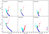 |
Fig. 1. Gaia EDR3 colour–magnitude diagrams of the studied clusters for stars with high membership probabilities, p ≥ 0.4 (see text for details). The different populations are plotted in different colours: RGB/RC (red), SGB (magenta), TO (green), MS (blue), candidate BSS (cyan squares), and candidate binaries (light grey). |
3. Radial density profiles
In order to investigate the spatial distributions of the stellar populations inside the studied clusters, it is necessary to remove projection effects, which are important in cases such as NGC 188 due to its location close to the north celestial pole. For this purpose, we computed projected Cartesian coordinates, x and y, using the Eq. (2) by Gaia Collaboration (2018b). In our case, we selected the cluster centre listed in Table 1 taken from Cantat-Gaudin et al. (2020) as the origin (α0, δ0). In this system, the x-axis is antiparallel to the right ascension (RA) axis, and the y-axis is parallel to the declination (Dec) axis. We used the distances to each cluster reported by Cantat-Gaudin et al. (2020) and listed in Table 1 to convert x and y coordinates into parsecs. Finally, the radial distance for each star was obtained from the Cartesian coordinates, defined above as  .
.
The spatial distributions of the studied clusters projected in the sky in Cartesian x and y coordinates are shown in Fig. 2, where the size of the points is proportional to their membership probability. The first noticeable feature is the tail towards the southeast of NGC 188, almost in the direction of motion marked by the arrow. Although without a clear tail, NGC 2420 and NGC 2425 show non-isotropic distributions in their outskirts. In the case of NGC 2425, the distribution appears to be aligned with the orbit. The other three clusters have a more regular distribution, but in the case of NGC 6819 the central region seems to be elongated in the SE–NW direction, again almost aligned with the movement, as already reported by Kamann et al. (2019).
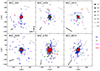 |
Fig. 2. Spatial distribution in Cartesian coordinates (x, y) of the studied cluster. The size of the points is proportional to the astrometric membership probability. The different populations are colour coded as in Fig. 1, excluding the binaries and BSSs for clarity. The dark grey arrows in the bottom left corner show the direction of motion and their length is proportional to the velocity in each axis. The light grey arrows in the top right corner show the direction to the Galactic centre. |
The radial density profile is the basic tool used to investigate the spatial distribution of stellar systems, such as open clusters, providing clues about their dynamical evolution. For the studied systems, we calculated the mean stellar surface density of objects within concentric rings as  , where Ni is the number of stars within the ith ring with an inner radius of Ri and an outer radius of Ri + 1. The density uncertainty in each ring was estimated assuming Poisson statistics.
The obtained radial density profiles are shown in Fig. 3. Only two of the studied clusters, NGC 188 and NGC 2682, show some hints of flattening in the outskirts. In contrast, for the other four systems, with a change of slope, the radial density profiles continue to fall until 150 pc, which may imply that we did not reach the end of the cluster.
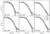 |
Fig. 3. Radial density profiles of the studied clusters. We overplot the best fits of the King (green dashed lines), Wilson (purple dot-dashed lines), LIMEPY (blue solid lines), and SPES (red solid lines) models. |
There are also some differences in the core regions. While some clusters show clear flat cores, such as NGC 6791, others show a cusp profile, such as NGC 2682 and, to a lesser degree, NGC 2420. In the case of NGC 2425, it seems that the core is smaller than in the other systems and its central region has been sampled with only two rings. The dichotomy of flat and cusp cores is well known in Galactic globular clusters (e.g. Djorgovski & King 1986; Trager et al. 1995). We discuss this issue in detail in Sect. 6.
3.1. LIMEPY models
The most direct way to interpret the observed radial density profiles is by comparison with the predictions of dynamical models. It is widely stated in the literature that, in spite of the irregular appearance of open clusters, their radial density profiles are well reproduced by isothermal and spherical King models (King 1966); with the exception of the outermost external regions, which require an additional power-law decrease term (e.g. Carrera et al. 2019b).
Davoust (1977) showed that the widely used King and Wilson (in the non-rotating and isotropic limit; Wilson 1975) models are particular cases of a more general family of models. These were extended to a more general class of (isotropic) lowered isothermal models by Gomez-Leyton & Velazquez (2014). Gieles & Zocchi (2015) further expanded them by introducing parametrised prescriptions for the energy truncation related to the edge of the cluster, and for the amount of radially biased pressure anisotropy, which determines the size of the isotropic cores. These latter authors introduced the Lowered Isothermal Model Explorer in PYthon (LIMEPY)2. These models are particularly suited to describing the phase-space density of stars in tidally limited, mass-segregated stellar clusters in all stages of their life cycle.
To identify one model within the LIMEPY family, it is necessary to specify the values of five parameters: the central dimensionless potential, W0; the anisotropy radius, ra; the truncation parameter, g; the total mass of the system, Mcl; and the half-mass radius, rh. The central dimensionless potential, W0, is used as a boundary condition to solve the Poisson equation, and it determines the shape of the radial profiles of some relevant quantities. The anisotropy radius is related to the amount of anisotropy present in the system: the smaller the radius, the more anisotropic the model is. The truncation parameter sets the sharpness of the truncation in energy: the larger it is, the more extended the models are, and the less abrupt the truncation is. When considering the isotropic version of the models, g = 0 corresponds to the Woolley (1954) models, g = 1 to the King (1966) models, and g = 2 to the non-rotating Wilson (1975) models. We added a sixth parameter, as suggested by Zocchi et al. (2016), to account for the background density: ρbg.
3.2. SPES models
As mentioned above, LIMEPY models are not able to reproduce the outermost radii sampled in each cluster. The LIMEPY models provide a more elaborate description of stars near the truncation, but do not include the effect of the Galactic tidal potential, unlike other models (e.g. Varri & Bertin 2009). The tidal field makes the potential in which the stars move anisotropic, and it slows down the escape of stars (Fukushige & Heggie 2000; Baumgardt 2001), because escape is limited to narrow apertures around the Lagrangian points. The result is the existence of a stellar population, known as potential escapers, which are energetically unbound, but have not yet escaped because they have not reached the Lagrangian points (e.g. Daniel et al. 2017). These objects are responsible for an elevation of the density and velocity dispersion near the Jacobi radius (Küpper et al. 2010; Claydon et al. 2017). The presence of potential escapers in globular clusters has been suggested to be responsible for the peculiarities observed in their outskirts.
These “spherical potential escapers stitched” (SPES; Claydon et al. 2019) models have an energy truncation similar to that of the LIMEPY models discussed above, with the fundamental difference that the density of stars at the truncation energy can be non-zero. More importantly, the SPES models include stars above the escape energy, with an isothermal distribution function that continuously and smoothly connects to the bound stars.
Apart from W0, Mcl, and rh, the SPES models depend on two additional parameters, B and η. The value of B can be 0 ≤ B ≤ 1, where B = 1 implies that there are no potential escapers. The parameter η is the ratio of the velocity dispersion of the potential escapers to the velocity scale, and can have values 0 ≤ η ≤ 1. For η = 0, there are no potential escapers. For fixed B, the fraction of potential escapers correlates with η. For fixed η, the fraction of potential escapers anticorrelates with B when B is close to 1. For small values of B, the fraction of potential escapers is approximately constant or loosely correlates with B at η constant. Finally, in the presence of potential escapers the SPES models are not continuous at the tidal radius, rt, but they have the ability to be solved (continuously and smoothly) beyond rt to mimic the effect of escaping stars (see Claydon et al. 2019, for a detailed discussion).
3.3. Model fits
In order to fit the observed radial density profiles with both LIMEPY and SPES models, we used a Bayesian approach following Zocchi et al. (2016) to determine the posterior probability distribution of the input parameters. For LIMEPY, we chose uniform priors over the following ranges: 0.8 < W0 < 15, 0.2 < g < 2.1, 0.1 < Mcl < 106 M⊙, 0.2 < rh < 30 pc, −1 < log ra < 3, and −8 < log ρbg < −1. In the case of the SPES models together with the values of W0, Mcl, and rh described above, we selected: 0 ≤ B ≤ 1 and 0 ≤ η ≤ 1. We used a Markov chain Monte Carlo fitting technique to explore the parameter space and to efficiently sample the posterior probability distribution for the parameters above from the LMFIT PYthon implementation3.
We considered the widely used King, g = 1, and the isotropic and non-rotating Wilson models, g = 2. These provide a fairly simple description of cluster morphology, with their shape being entirely determined by the dimensionless central potential W0. In this case, high values of W0 imply more concentrated models. The third case is the isotropic, single-mass LIMEPY models, which fit W0 and the truncation parameter g simultaneously. Finally, we fit the SPES models. In each case, we performed 500 realisations for each cluster.
3.4. Results
The best fits for King (green dashed lines), Wilson (purple dot-dashed lines), LIMEPY (blue solid lines), and SPES (red solid lines) models are shown in Fig. 3. The corresponding parameters are listed in Tables 2–4 for King, Wilson, LIMEPY, and SPES models, respectively. Individual fits, together with their uncertainty ranges, are shown in Figs. C.1–C.4, respectively.
Best-fitting parameters of King, g = 1, and Wilson, g = 2, LIMEPY models.
Best-fitting parameters of LIMEPY models.
Best-fitting parameters of SPES models.
As expected, LIMEPY models – not only in the specific King and Wilson prescriptions but also the general ones – are not able to reproduce the outskirts of the observed radial density profiles (Fig. 3). The SPES models reproduce the profiles at large radii thanks to the inclusion of potential escapers, which are those with the lowest χ2 values. The only exception is NGC 188 for which the fit of the LIMEPY model produced a slightly lower χ2 than the SPES ones. In any case, none of the models used are able to reproduce the cusp core observed in NGC 2682 or even the weaker cusp core in NGC 2420. On the contrary, they reproduce the flat core of NGC 6791 and the intermediate region between the core and the tidal radius quite well for all the studied systems (Fig. 3).
In general, the simple King and Wilson models produce larger χ2 values than the general LIMEPY models, without significant differences among them except in the outskirts. The smooth variation between the King and Wilson models, and also the Woolley ones, is controlled by the variation of the truncation parameter. In our case, we find that the majority of the studied clusters are close to the King models with g ∼ 1, contrary to what was reported by de Boer et al. (2019) for globular clusters, with values close to the Wilson template. The individual King models better reproduce the cluster profiles in four cases, while the Wilson ones work better for NGC 2425 and NGC 6819. This may be due to the fact that these systems are relatively more extended than others. In conclusion, King models are a good first approximation of the open cluster density profiles, especially if the external regions are excluded.
A key parameter in the LIMEPY models is the anisotropy parameter, ra. We find large values of ra for all the studied clusters, which implies that the amount of anisotropy in them is quite low. The only exception is NGC 6791 for which we find a very low value of ra. About the half mass radius, rh, which encloses half of the total mass of the system, the SPES model values are slightly lower than those of the LIMEPY ones; with the exception of NGC 188, for which the best LIMEPY model has a slightly lower value than that of the best SPES model. In both cases, the lowest value is obtained for NGC 188. Concerning the masses, we also find that the LIMEPY models produce slightly larger values than the SPES ones. This is explained by the fact that the SPES models consider that a fraction of observed stars are unbound to the systems, which means that the amount of mass needed is lower. The obtained masses may be considered as a lower limit on the real value. Owing to the fact that we have a magnitude limit, G ≤ 18.5 mag, we do not sample the faintest objects, which have a particularly striking effect on the furthest object, NGC 6791. Using a different magnitude threshold, we verified that the derived masses were comparable, while there are objects below the turn-off, such as one magnitude, but they decrease when the limit is around the turn-off or above it. Moreover, we excluded binaries and blue stragglers stars from this analysis.
The core radius, rc, and truncation or tidal radius, rt, are not obtained from the fits, but they are computed as a function of the best results for both LIMEPY and SPES models, respectively. Derived core radii for both families of models are similar, showing the same trend: the LIMEPY model values are slightly larger than those of the SPES models, again with the exception of NGC 188. NGC 6791 shows the largest rc, while NGC 2425 has the smallest one. Tidal radii show a similar tendency. However, the values derived for LIMEPY models are very different among clusters, from the 28.8 pc of NGC 188 to the 416 pc of NGC 6819. Only NGC 188 and NGC 2682 show a flattening in the outermost radii studied, most probably due to the algorithm not being able to properly place the end of the cluster. On the contrary, the SPES models provide smaller tidal radii, of between 25 pc for NGC 2420 and 55 pc for NGC 188. This implies that the objects located outside these radii are extra-tidal stars, which are probably escaping from the clusters. According to SPES models, between 13% (for NGC 188) and 23% (for NGC 2425) of the observed stars in each system may have sufficient energy to escape from them.
Other works have studied the radial density profiles of the clusters in our sample, mainly by fitting them with the analytical King profile model. The majority of these studies were performed in recent years, taking advantage of the different Gaia data releases (Gao 2018; Gao & Fang 2022; Zhong et al. 2022; Angelo et al. 2023; Cordoni et al. 2023). Together with the variety of algorithms used to calculate the membership probabilities, the main distinguishing factor of our study is the area studied around the cluster centre, which is significantly larger than in the majority of previous studies. In general, the values for the core radius reported by these works are of the order of or slightly smaller than the values found here. There are larger discrepancies in the tidal radius determination. This is explained in part by the relatively small area covered by several of these works, and by the presence of unbound stars, in the same way as the differences found above between LIMEPY and SPES models. To our knowledge, the recent work by Angelo et al. (2023) is the only one that derived masses for the studied clusters, four of which are in common with our sample: NGC 188, NGC 2682, NGC 6791, and NGC 6919. Using a different approach, the masses derived for these clusters are in good agreement – within the uncertainties – with the ones obtained here from the LIMEPY models.
4. Mass segregation
It has been widely reported in the literature that old open clusters are segregated in mass (e.g. Mathieu 1984), with massive objects concentrated in the central region and low-mass stars dispersed in the outskirts. In spite of some evidence of primordial mass segregation in very young massive clusters (e.g. Kim et al. 2006; Stolte et al. 2006), in old open clusters this should be a direct consequence of their internal dynamics.
In order to investigate the mass segregation of the studied clusters, we obtained the cumulative projected radial distribution of the different stellar populations normalised to the total number of the objects in each of them. In spite of the uncertainties in our membership determinations for BSSs and binaries, we included both populations in our analysis (see Carrera et al. 2019b, for details). According to Fig. 4, all the studied clusters are segregated in mass, with the RGB more concentrated than the less massive objects in the MS. The only exception is the central part of NGC 6791, as within the innermost 2 pc there is no clear separation among the different stellar populations. Mass segregation has already been reported in the literature for the majority of the studied clusters, mostly based on membership determination from the pre-Gaia era: NGC 188 (e.g. Bonatto et al. 2005; Geller et al. 2008), NGC 2420 (e.g. Leonard 1988; Peikov et al. 2002; Paparo 1982), NGC 2682 (e.g. Balaguer-Núñez et al. 2007; Geller et al. 2015; Gao 2018, NGC 6791 (e.g. Gao 2020; Platais et al. 2011), and NGC 6819 (e.g. Kalirai et al. 2001; Kang & Ann 2002; Yang et al. 2013). In general, the global distributions are mainly due to the MS stars, whereas TO and SGB objects are more concentrated. To quantify this statement, we computed the radii containing 15% and 85% of each population (Table 5). The concentration of the different populations changes from one cluster to another. For example, in the case of NGC 2682, the more massive RGB and SGB stars are notoriously more concentrated towards the innermost parts than the other populations. It seems that in the case of NGC 188, the TO objects are more concentrated than RGB and SGB objects. This could be explained by the fact that, for NGC 188, the mass difference between RGB and MS TO objects should be lower than in the case of NGC 2682, as NGC 188 is about 4 Ga older. For NGC 2420, there is a non-negligible number of binaries in the outermost radii. Finally, the SGB population in NGC 2425 exhibits an unexpected behaviour, flattening between ∼1 and 10 pc; however, this could be an effect due to low-number statistics.
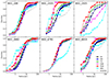 |
Fig. 4. Cumulative projected radial distribution of the different populations identified in each of the clusters normalised to the total number of stars in each population. Error bars are not plotted for clarity. |
Summary of cumulative projected radial distribution of different populations.
Particularly interesting is the case of the BSSs, which are typically more concentrated than even the RGB stars. The mechanisms for the formation of BSSs are still not fully understood. These stars are thought to derive from normal MS stars that have increased in mass above a single star mass typical of the turn-off through mass transfer, mergers (e.g. McCrea 1964; Paczyński 1971), or collisions in binary systems (e.g. Hills & Day 1976). As reported by Carrera et al. (2019b), these objects show a bimodal distribution in the majority of the studied clusters, as observed in globular clusters (e.g. Ferraro et al. 1997; Lanzoni et al. 2007) and predicted by dynamical simulations (e.g. Mapelli et al. 2004).
In order to quantify and compare the degree of mass segregation among the studied clusters, we used the method proposed by Allison et al. (2009), which consists of comparing the lengths of the minimum spanning tree (MST) of the most massive stars of a cluster and a set of the same number of randomly chosen objects between all populations. An MST of a set of points is the path connecting all the points, with the shortest possible path length and without any closed loops. In a given set of points, only one MST can be drawn. In our case, we defined the mass-segregation ratio (MSR) as:
 (1)
(1)
where ⟨lrandom⟩ and ⟨lmassive⟩ are the average lengths of the MST of N randomly selected stars between all and massive samples, respectively. The average lengths ⟨lrandom, massive⟩ are calculated over 100 iterations, where at each iteration, we drew a different subsample of random stars allowing us to simultaneously calculate σrandom, massive, the standard deviation of the lengths of the MST. We computed the uncertainty of ΛMSR as the square root of the quadratic sum of σrandom and σmassive.
We computed the MST using the csgraph routine implemented in the scipy PYthon module (Virtanen et al. 2020). We consider the RGB sample as representative of the massive stellar population in each cluster. After several trials, we assumed N = 15 stars. In principle, a ΛMSR greater than one means that the massive population is more concentrated than a random sample, and therefore that the cluster shows signs of mass segregation. The obtained values are listed in the last column of Table 5. In all the studied clusters, the red giants are more concentrated than random selected stars. Noticeable are the larger values found for NGC 2420 and NGC 2425, which are the least massive clusters in our sample (see Table 4) and are also among the youngest, where a larger mass difference between giants and unevolved stars is expected. On the other hand, the most massive systems have lower ΛMSR values. Indeed, the lowest value is found for the most massive system in our sample, NGC 6791, according to the results of the previous section; although this is also the furthest cluster, which implies that our sample only includes members in the upper MS, and therefore we are not sampling as many low-mass stars as in other clusters.
5. Physical parameters of the clusters
5.1. Half-mass relaxation time
The dynamical evolution inside the clusters is related to the encounters among stars. After losing a certain number of members, the relaxation time is the moment at which the stellar system reaches equilibrium. In other words, this is also defined as the time required for a star to lose the memory of its initial conditions. The relaxation time is locally defined, and it can vary by several orders of magnitude in different regions of a single cluster. For this reason, the relaxation time is widely calculated in reference to the system’s half-mass radius, the so-called half-mass relaxation time, trh.
The half-mass relaxation time can be derived according to McLaughlin & van der Marel (2005) as:
![Mathematical equation: $$ \begin{aligned} t_{\rm rh}[a]=\left[\frac{2.06\times 10^6}{\ln {\frac{0.4 M_{\rm cl}}{m_*}}}\right]m_*^{-1} M_{\rm cl}^{1/2}r_{\rm h}^{3/2}, \end{aligned} $$](/articles/aa/full_html/2024/07/aa48220-23/aa48220-23-eq10.gif) (2)
(2)
where Mcl and rh are expressed in M⊙ and parsecs, respectively. In this section, we consider only the values derived from the SPES models because these latter better reproduce the radial density profiles in comparison to the LIMEPY models. The average current stellar mass in the cluster, m*, is defined as Mcl/Ncl, where Ncl is the number of stars in the cluster. Assuming the Kroupa (2001) initial mass function, m* has a value of 0.54 M⊙. Considering that the most massive stars have already died, we assume m* ∼ 0.5 ± 0.1 M⊙ to allow for some deviation. The obtained values are listed in Table 6 together with their dynamical ages τrh = logage/trh.
Physical properties obtained using cluster masses derived from SPES models.
Recently, Angelo et al. (2023) determined the half-mass relaxation time for a sample that includes four systems in common with ours. Except those for NGC 6791, our values are larger than those derived by Angelo et al. (2023) for the four clusters in common, which is mainly caused by the fact that we are using larger input cluster masses and half-mass radii, since our study covers a wider area and contains a larger number of members.
5.2. Jacobi radius
Stellar clusters do not live in isolation, but are orbiting the Galaxy inside its tidal field. The Jacoby radius, RJ, – also referred to as the Hill or Roche radius – of a stellar cluster is the maximum distance inside which a star is still bound gravitationally to the system taking into account the external Galactic tidal potential. Therefore, it can be considered as a prediction of the tidal radius. According to King (1962), RJ can be derived as:
 (3)
(3)
where Rp is the perigalactic radius defined as Rp = Rapo(1 − e), where Rapo and e are the apocentre radius and the eccentricity of the cluster orbit, and Mcl and Mg are the mass of the cluster and that of the Galaxy enclosed within the orbit of each cluster, respectively.
We use the orbital parameters determined by Carrera et al. (2022) – except for NGC 2425 for which we assume the values determined by Tarricq et al. (2021). In both cases, the cluster orbits were computed using the galpy package (Bovy 2015). In order to determine the mass enclosed within the orbit of each system, Mg, which is model dependent, we also took advantage of the galpy package, assuming the MW2014 potential for the Milky Way (see Bovy 2015, for details).
The derived Jacobi radii are listed in Table 6. Using other potentials available in the literature, such as that of McMillan (2017), yields similar values. Increasing the mass of the clusters, for example using the values derived from LIMEPY models, yields slightly larger Jacobi radii. On the other hand, an increase in the Galaxy mass enclosed inside the cluster orbit tends to reduce RJ.
Alternatively, the Jacobi radius can be derived from the tidal tensor of the total potential (Renaud et al. 2011). In general, the values derived using this latter method are lower than those derived here, except for the case of NGC 6791. This discrepancy may be due to the fact that our masses, from SPES models, are larger than those derived by Angelo et al. (2023). In any case, neither our RJ estimations nor those of Angelo et al. (2023) are as large as the tidal radius determined by both SPES and LIMEPY models.
5.3. Initial mass
A stellar cluster loses mass mainly because of stellar evolution and tidal disruption. Lamers et al. (2005a) showed that the fraction of the cluster initial mass, Mini, lost because of stellar evolution, (ΔM)ev, in the GALEV (Galaxy Evolutionary Synthesis, Kotulla et al. 2009) models can be written as  , which can be approximated as:
 (4)
(4)
where aev, bev, and cev are coefficients that depend to a small extent on metallicity according to Table 1 of Lamers et al. (2005a). Metallicities are obtained from iron abundances using the values provided by Carbajo-Hijarrubia et al. (in prep.); except for NGC 2425, which was obtained from Randich et al. (2022).
More generally, the evolution with time of the mass of a cluster that has survived infant mortality, and has an age of ≥107 a, can be described as:
 (5)
(5)
where the first term describes mass loss due to stellar evolution and the second that due to disruption.
The mass decrease of a cluster can be approximated very accurately as:
![Mathematical equation: $$ \begin{aligned} \mu (t; M_{\rm ini}) \equiv \frac{M_{\rm cl}}{M_{\rm ini}} \sim \left\{ \left[ \mu _{\rm ev}(t) \right]^{\gamma } - \frac{\gamma }{M^{\gamma }_{\rm ini}} \frac{t}{t_0}\right\} ^{1/\gamma }, \end{aligned} $$](/articles/aa/full_html/2024/07/aa48220-23/aa48220-23-eq15.gif) (6)
(6)
where masses are expressed in M⊙, μev(t) = 1 − qev(t), and γ = 0.62 according to Lamers et al. (2005a). The constant t0 depends on the galaxy potential in which the cluster is moving, and on the eccentricity, e, of its orbit. From Lamers et al. (2005b), it can be derived from:
 (7)
(7)
where Cenv, 0 = 810 Ma for the Milky Way (see Lamers et al. 2005b, for details), and ρamb is the ambient pressure evaluated at the position of the cluster, expressed in M⊙ pc−3. This latter was determined for each cluster with the galpy package, assuming the MW2014 potential (Bovy 2016).
The initial cluster mass can be easily derived by manipulating Eq. (6) as:
 (8)
(8)
The obtained Mini values are listed in Table 6. In comparison with Angelo et al. (2023), who determined initial masses following a similar procedure, our estimations are slightly larger, except for NGC 6791, the most massive system in our sample, which is significantly smaller. Together with the different input cluster masses, the only difference between the two studies is related to the treatment of the Galaxy tidal field.
Finally, Baumgardt & Makino (2003) found that the disruption time of a stellar cluster can be expressed as a function of Mini as  with tdis in years. The derived values are also listed in Table 6. The values we obtain for the disruption time of the clusters analysed here are discussed in the following section.
6. Physical interpretation
6.1. Dynamical evolutionary stages
We discuss the dynamical stages of the studied clusters as a function of the derived structural parameters (rh, rt, rc), relaxation times (τrh), Jacobi radii (RJ), location in the disc (Rgc, Z), and evolution-related parameters (age and stellar mass). Our results are summarised in the different panels of Fig. 5. In order to compare to the global trends described by open clusters, we also plot the results obtained by Angelo et al. (2023). These authors studied four of the clusters in our sample: NGC 188, NGC 2682, NGC 6791, and NGC 6819. We recovered slightly large structural parameters in relation to the results of Angelo et al. (2023), mainly due to the fact that we are covering a relatively large area around the clusters. In either case, the results obtained for these systems, mainly the ratios among the different radii, are compatible within the uncertainties.
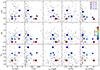 |
Fig. 5. rh/RJ (top), rt/RJ (middle), and rt/rc (bottom) as a function of Rgc, Z, τrh, Mcl/Mini, and cluster mass. The clusters studied here are labelled with different colours as a function of age, and are marked with symbols to facilitate their identification. Grey dots are the clusters studied by Angelo et al. (2023). |
The two oldest clusters in our sample, NGC 188 and NGC 6791, are also the most dynamically evolved systems according to their dynamical ages, τrh > 0.7 dex. These systems have galactocentric distances of between 8 and 9 kpc from the centre of the Galaxy; they are located more than 500 pc above the Galactic plane, and are therefore less affected by the destructive influence of the disc. This is in agreement with the idea that clusters of similar ages are preferentially located outside the dense disc, which may play a role in their survival (e.g. Friel 2013; Cantat-Gaudin et al. 2020). These two systems also have the lowest rt/rc, which can be explained by the fact that they have reduced in size throughout their lives by losing a significant part of their outskirts. The remnants that we observe today are mainly the cores of the earlier clusters. This hypothesis is supported by the fact that they have lost more than 70% of their birth mass. Moreover, these two systems show the lowest mass segregation ratios, ΛMSR. This can be a consequence of the fact that they have lost a significant fraction of their least massive stellar components. They also show the lowest rh/RJ and rt/RJ ratios, implying that they are well inside their Jacoby radius. This would mean that their evolution is mainly dominated by their internal dynamics and not by the influence of the Galactic tidal potential. This result is in agreement with the N-body simulation’s prediction that cluster that underfill their Roche lobe will survive a number of relaxation times (e.g. Gieles & Baumgardt 2008).
NGC 6819 is a 1.9 Ga old and very massive system, Mcl = 19 × 103 M⊙, located at 8 pc from the Galactic centre. It has lost less than 50% of its initial mass. NGC 2682 is older, 3.6 Ga, but is less massive and is located at a similar height above the Galactic plane but about 1 kpc further, and has lost a somewhat larger fraction of its birth mass, that is, ∼60%. NGC 2682 is slightly more concentrated, which may mean that this cluster is more dynamically evolved, as evidenced by its dynamical age. In spite of their significantly different initial and present masses, the two systems have similar dissolution times because of the fact that the most massive one is also located at an inner galactocentric distance.
On the other hand, NGC 2420, which has almost the same age as NGC 6819, is located much further out, Rgc = 10.7 kpc, and also at a larger distance from the plane, Z = 869 pc, than NGC 2682 and NGC 6819. This cluster is twice and four times less massive than NGC 2682 and NGC 6819, respectively. However, its dissolution time is only a little lower, mainly because of its location. These three clusters have similar rt/RJ ratios of about 0.8, which means that they occupy almost their entire Roche volume, and therefore their dynamical evolution is modulated by the Galactic tidal field.
Finally, NGC 2425 is the furthest cluster in our sample but is also the closest to the Galactic plane. It has an age similar to those of NGC 2420 and NGC 6819. This cluster shows clear hints of dissolution. On one hand, it has a rt/RJ ratio of larger than one, meaning that it completely fills its Roche volume; it may have been more exposed to external tidal forces (e.g. Ernst et al. 2015). It is also the system with the lowest concentration, which may mean that the stars that form this system are more weakly gravitationally bound. We note that we find a significantly larger fraction of potential escapers for NGC 2425 than for the other clusters in our sample. However, NGC 2425 is coeval, was formed with a similar initial mass, and is located at a similar galactocentric distance to NGC 2420; it has lost a significantly larger fraction of its mass because of its shorter distance to the galactic plane. Taking into account its age, NGC 2425 will dissolve in about 2.5 Ga from now.
Although our work is based on a small sample of only six clusters, we can obtain valuable conclusions, which should nevertheless be confirmed with larger samples. Our results reinforce the idea that initial mass and location in the Galaxy – mainly above or below the disc – play a fundamental role in the survival of open clusters. Those systems that do not completely fill their Roche volumes may survive longer; either they were born more concentrated or they lost a significant fraction of their outskirts. Furthermore, our results suggest that the concentration of the cluster increases with age.
6.2. Disc-crossing times
In Sect. 3 we report the existence of tails in several of the studied clusters, such as NGC 188. In order to investigate the influence of the Galactic plane on the morphology of the studied systems, we estimated the last disc crossing. For this purpose, we used the orbits determined by Carrera et al. (2022) for all clusters except NGC 2425, for which we used that of Tarricq et al. (2021). In both cases, the orbits were derived using the PYthon galpy package (Bovy 2015) and the MW2014 potential. We refer the reader to the original papers for further details. We did not attempt to derive new orbits, because the available values are the same, within the uncertainties, as those used in the orbit determination.
The times of the last disc crossing of each cluster are listed in the last column of Table 6. NGC 6819 crossed the disc very recently, that is, only about 12 Ma ago, which may explain its elongation. Moreover, it has a relatively high disc-pass frequency, as it crosses the disc about every 50 Ma. Among the other clusters, NGC 6791 passed the disc about 26 Ma ago, but there is no sign of elongation. The remaining clusters crossed the plane more than 30 Ma ago. We note that the largest value is obtained for NGC 2425 but since this cluster does not reach a significant distance from the plane, its orbit is embedded inside the disc, and therefore the last disc crossing is not relevant.
In order to evaluate this impact, we computed the slopes of the radial density profiles of the studied clusters simply using a linear least square fitting. The results are shown in Fig. 6. Although the uncertainties in these external regions are large due to the small number of stars sampled, there is a hint of a correlation between the slope of the external region and the time that the clusters crossed the disc for the last time, with no clear relation to the actual distance from the Galactic plane. However, due to the small number of systems in our sample, this result should be confirmed with larger samples.
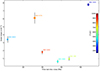 |
Fig. 6. Slope of the outermost region of the radial density profile as a function of the last time the clusters crossed the disc. The clusters are colour coded as a function of their actual distance to the Galactic plane and the same symbols are used as in previous figures. |
6.3. A cusp–core dichotomy for open clusters?
There are also clear differences between the radial density profiles of the central regions of the studied clusters. In principle, these central regions are less affected by external perturbations, and therefore they may be dominated by the gravitational encounters of their members (e.g. O’Leary et al. 2014). A direct consequence of two-body relaxation is the redistribution of the stars, the mass segregation, and modification of their velocities due to the exchange of energy and angular momentum. We note that the ages of the studied clusters are at least twice their trh and therefore the two-body relaxation has had sufficient time to act. All the clusters show clear signs of mass segregation, particularly in their cores, with mass segregation ratios, ΛMSR, of larger than two. Exceptions are NGC 188 and NGC 6791, with the lowest mass segregation ratios, which, as discussed above, should be related to the fact that these systems have lost a significant fraction of their least massive members.
Interestingly, the clusters with the lowest ΛMSR values show flat profiles in their central regions, which is particularly clear in the case of NGC 6791. Meanwhile, for systems with higher values, a power-law increase is apparent, the so-called cusp profile, which is especially clear in the case of NGC 2682. From our limited sample, the systems with a larger dynamical age show a core morphology.
The cusp–core dichotomy in the central density profiles is well known among the globular clusters, which are more massive and older than open clusters (e.g. McLaughlin & van der Marel 2005). Although there are still gaps in our knowledge of the mechanisms responsible for the cuspy profiles, it is widely assumed that clusters with such profiles have experienced complex internal dynamics (e.g. Meylan & Heggie 1997); they are associated with systems that have suffered a gravothermal collapse, in which the increase in the central density becomes dramatic, and is known as core collapse (Lynden-Bell & Wood 1968). However, the timescale over which this increase takes place is shorter than in the case of globular clusters, and so the oldest open systems could have experienced it (Spitzer 1987).
For globular clusters, several features have been related to cusp systems in comparison with core ones, such as a higher central density, a large binary fraction, a significant BSS population, and a high number of X-ray sources (e.g. Meylan & Heggie 1997). Binary fractions of between 20% and 40% have been reported in the literature for the clusters in our sample (e.g. Bedin et al. 2008; Milliman et al. 2014; Thompson et al. 2021), but this value becomes 70% ± 17% for the central region of NGC 2682 (Geller et al. 2021), and is 32% ± 3% for NGC 6791 (Bedin et al. 2008). However, Rain et al. (2021) reported the largest BSS populations for NGC 6791 and NGC 188 with 48 and 22 objects, respectively. NGC 2420, NGC 2682, and NGC 6819 contain 3, 11, and 15 BSSs, respectively (Rain et al. 2021). These numbers are in agreement with our results, although our procedure is not the most appropriate for these stars. X-ray observations in the literature suggest that NGC 2682 contains between two and seven times more active binaries – when normalised to the cluster mass – than NGC 6791, and even more with respect to NGC 6819 (van den Berg et al. 2013).
On the other hand, cored profiles can be a sign of the existence of massive remnants in the cluster centres, such as stellar-mass black holes (e.g. Merritt et al. 2004). Their presence is able to prevent the segregation of the mass of the host systems in their central regions (e.g. Peuten et al. 2016). Initially, the formation of black holes in open clusters was discarded because of their low densities. However, recent dynamical studies have demonstrated that binary black holes can form in open clusters by different mechanisms (e.g. Mapelli 2016; Kumamoto et al. 2020). Indeed, very recently, Torniamenti et al. (2023) proposed the existence of a black hole population to properly reproduce the density profile of the Hyades open cluster.
7. Summary and conclusions
In this study, we determined membership probabilities from Gaia astrometry for stars in the field of view of six of the oldest open clusters in the Milky Way in order to investigate their longevity: NGC 188, NGC 2420, NGC 2425, NGC 2682, NGC 6791, and NGC 6819. From our study of their spatial distributions, we find that NGC 188 shows signs of a tail; NGC 2425 exhibits a non-isotropic distribution of the external region; and an elongation of the central region can be seen for NGC 6819. These structures are aligned with the directions of motion of the respective cluster.
The derived radial density profiles show some signs of flattening in the outskirts for two of the clusters, NGC 188 and NGC 2420. For the other clusters, we only observe a change in the slope. There are also significant differences in the central regions. While NGC 2682 shows a power-law density increase – the so-called cusp profile –, NGC 6791 exhibits a flat profile, otherwise known as a core profile.
We use LIMEPY and SPES models to characterise the observed radial density profiles. A fraction of potential escapers – that is, stars with sufficient energy to leave the system or already be outside of it – is needed to properly reproduce the external regions. These models are used to determine some of the properties of the clusters, such as their current masses, or their half-mass, tidal, and core radii. We find that the studied clusters are more extended than previously reported in the literature.
We discuss the obtained results, also taking into account the influence of the Galaxy. A high initial mass is needed to survive, but also the location in the Galaxy plays a role in the clusters’ longevity – with larger distances from the Galactic plane being advantageous to survival. The most dynamically evolved systems do not completely fill their Roche volumes and have lower rt/rc ratios. Moreover, all the cluster are segregated in mass but the most dynamically evolved clusters show lower mass segregation ratios, which is likely to be explained by the fact that these systems have lost a significant fraction of their least massive members.
Finally, the observed cusp–core dichotomy in the central regions may be related to different dynamical evolution. As in the case of globular clusters, cusp profiles may be related to more complex dynamical evolutions, with a large presence of binaries and X-ray emission. On the other hand, the presence of massive remnants, such as black holes, would prevent the mass segregation and formation of cusp profiles. More data – mainly kinematical – are needed to verify these hypotheses. These will be provided by Gaia for the brightest targets and by massive spectroscopic surveys for the fainter ones.
LIMEPY is available from https://github.com/mgieles/limepy
LMFIT is available at https://lmfit.github.io/lmfit-py/
Acknowledgments
We acknowledge the anonymous referee for his/her very constructive comments, which have contributes to increase the quality of this paper. N.A.-B. acknowledges the RECA (Red de Estudiantes Colombianos en Astronomía – Network of Colombian astronomy students) internship programme for the opportunity to begin this work. H.T. was funded under the Erasmus+ 2020 programme of the European Commission. This work was supported by the MINECO (Spanish Ministry of Economy, Industry and Competitiveness) through grant ESP2016-80079-C2-1-R (MINECO/FEDER, UE) and by the Spanish MICIN/AEI/10.13039/501100011033 and by “ERDF A way of making Europe” by the “European Union” through grants RTI2018-095076-B-C21 and PID2021-122842OB-C21, and the Institute of Cosmos Sciences University of Barcelona (ICCUB, Unidad de Excelencia “María de Maeztu”) through grant CEX2019-000918-M. This work has made use of data from the European Space Agency (ESA) mission Gaia (https://www.cosmos.esa.int/gaia), processed by the Gaia Data Processing and Analysis Consortium (DPAC, https://www.cosmos.esa.int/web/gaia/dpac/consortium). Funding for the DPAC has been provided by national institutions, in particular the institutions participating in the Gaia Multilateral Agreement.
References
- Allison, R. J., Goodwin, S. P., Parker, R. J., et al. 2009, MNRAS, 395, 1449 [Google Scholar]
- Angelo, M. S., Santos, J. F. C., Maia, F. F. S., & Corradi, W. J. B. 2023, MNRAS, 522, 956 [NASA ADS] [CrossRef] [Google Scholar]
- Balaguer-Núñez, L., Galadí-Enríquez, D., & Jordi, C. 2007, A&A, 470, 585 [NASA ADS] [CrossRef] [EDP Sciences] [Google Scholar]
- Bally, J. 2016, ARA&A, 54, 491 [Google Scholar]
- Bastian, N., & Gieles, M. 2008, in Mass Loss from Stars and the Evolution of Stellar Clusters, eds. A. de Koter, L. J. Smith, & L. B. F. M. Waters, ASP Conf. Ser., 388, 353 [NASA ADS] [Google Scholar]
- Baumgardt, H. 2001, MNRAS, 325, 1323 [NASA ADS] [CrossRef] [Google Scholar]
- Baumgardt, H., & Makino, J. 2003, MNRAS, 340, 227 [NASA ADS] [CrossRef] [Google Scholar]
- Bedin, L. R., Salaris, M., Piotto, G., et al. 2008, ApJ, 679, L29 [CrossRef] [Google Scholar]
- Bertelli Motta, C., Pasquali, A., Caffau, E., & Grebel, E. K. 2018, MNRAS, 480, 4314 [NASA ADS] [CrossRef] [Google Scholar]
- Binney, J., & Tremaine, S. 2008, Galactic Dynamics: Second Edition (Princeton: Princeton University Press) [Google Scholar]
- Bonatto, C., Bica, E., & Santos, J. F. C. 2005, A&A, 433, 917 [NASA ADS] [CrossRef] [EDP Sciences] [Google Scholar]
- Bossini, D., Vallenari, A., Bragaglia, A., et al. 2019, A&A, 623, A108 [NASA ADS] [CrossRef] [EDP Sciences] [Google Scholar]
- Bovy, J. 2015, ApJS, 216, 29 [NASA ADS] [CrossRef] [Google Scholar]
- Bovy, J. 2016, ApJ, 817, 49 [NASA ADS] [CrossRef] [Google Scholar]
- Bragaglia, A., Tosi, M., Andreuzzi, G., & Marconi, G. 2006, MNRAS, 368, 1971 [NASA ADS] [CrossRef] [Google Scholar]
- Cantat-Gaudin, T., Vallenari, A., Sordo, R., et al. 2018a, A&A, 615, A49 [NASA ADS] [CrossRef] [EDP Sciences] [Google Scholar]
- Cantat-Gaudin, T., Jordi, C., Vallenari, A., et al. 2018b, A&A, 618, A93 [NASA ADS] [CrossRef] [EDP Sciences] [Google Scholar]
- Cantat-Gaudin, T., Anders, F., Castro-Ginard, A., et al. 2020, A&A, 640, A1 [NASA ADS] [CrossRef] [EDP Sciences] [Google Scholar]
- Carrera, R., & Pancino, E. 2011, A&A, 535, A30 [NASA ADS] [CrossRef] [EDP Sciences] [Google Scholar]
- Carrera, R., Bragaglia, A., Cantat-Gaudin, T., et al. 2019a, A&A, 623, A80 [NASA ADS] [CrossRef] [EDP Sciences] [Google Scholar]
- Carrera, R., Pasquato, M., Vallenari, A., et al. 2019b, A&A, 627, A119 [NASA ADS] [CrossRef] [EDP Sciences] [Google Scholar]
- Carrera, R., Casamiquela, L., Carbajo-Hijarrubia, J., et al. 2022, A&A, 658, A14 [NASA ADS] [CrossRef] [EDP Sciences] [Google Scholar]
- Casamiquela, L., Tarricq, Y., Soubiran, C., et al. 2020, A&A, 635, A8 [NASA ADS] [CrossRef] [EDP Sciences] [Google Scholar]
- Charbonnel, C., Lagarde, N., Jasniewicz, G., et al. 2020, A&A, 633, A34 [NASA ADS] [CrossRef] [EDP Sciences] [Google Scholar]
- Claydon, I., Gieles, M., & Zocchi, A. 2017, MNRAS, 466, 3937 [CrossRef] [Google Scholar]
- Claydon, I., Gieles, M., Varri, A. L., Heggie, D. C., & Zocchi, A. 2019, MNRAS, 487, 147 [NASA ADS] [CrossRef] [Google Scholar]
- Cordoni, G., Milone, A. P., Marino, A. F., et al. 2023, A&A, 672, A29 [NASA ADS] [CrossRef] [EDP Sciences] [Google Scholar]
- Daniel, K. J., Heggie, D. C., & Varri, A. L. 2017, MNRAS, 468, 1453 [NASA ADS] [CrossRef] [Google Scholar]
- Davoust, E. 1977, A&A, 61, 391 [NASA ADS] [Google Scholar]
- de Boer, T. J. L., Gieles, M., Balbinot, E., et al. 2019, MNRAS, 485, 4906 [Google Scholar]
- Djorgovski, S., & King, I. R. 1986, ApJ, 305, L61 [Google Scholar]
- Efron, B. 1982, The Jackknife, the Bootstrap and Other Resampling Plans (Philadelphia: Society for Industrial and Applied Mathematics) [Google Scholar]
- Ernst, A., Berczik, P., Just, A., & Noel, T. 2015, Astron. Nachr., 336, 577 [NASA ADS] [CrossRef] [Google Scholar]
- Fabricius, C., Luri, X., Arenou, F., et al. 2021, A&A, 649, A5 [NASA ADS] [CrossRef] [EDP Sciences] [Google Scholar]
- Ferraro, F. R., Paltrinieri, B., Fusi Pecci, F., et al. 1997, A&A, 324, 915 [NASA ADS] [Google Scholar]
- Friel, E. D. 2013, in Planets, Stars and Stellar Systems. Volume 5: Galactic Structure and Stellar Populations, eds. T. D. Oswalt, & G. Gilmore (Dordrecht: Springer Netherlands), 5, 347 [NASA ADS] [Google Scholar]
- Fukushige, T., & Heggie, D. C. 2000, MNRAS, 318, 753 [CrossRef] [Google Scholar]
- Gaia Collaboration (Brown, A. G. A., et al.) 2018a, A&A, 616, A1 [NASA ADS] [CrossRef] [EDP Sciences] [Google Scholar]
- Gaia Collaboration (Helmi, A., et al.) 2018b, A&A, 616, A12 [NASA ADS] [CrossRef] [EDP Sciences] [Google Scholar]
- Gaia Collaboration (Brown, A. G. A., et al.) 2021, A&A, 649, A1 [NASA ADS] [CrossRef] [EDP Sciences] [Google Scholar]
- Gaia Collaboration (Vallenari, A., et al.) 2023, A&A, 674, A1 [NASA ADS] [CrossRef] [EDP Sciences] [Google Scholar]
- Gao, X. 2018, ApJ, 869, 9 [NASA ADS] [CrossRef] [Google Scholar]
- Gao, X. 2020, Ap&SS, 365, 24 [NASA ADS] [CrossRef] [Google Scholar]
- Gao, X., & Fang, D. 2022, Ap&SS, 367, 87 [NASA ADS] [CrossRef] [Google Scholar]
- Geller, A. M., Mathieu, R. D., Harris, H. C., & McClure, R. D. 2008, AJ, 135, 2264 [Google Scholar]
- Geller, A. M., Latham, D. W., & Mathieu, R. D. 2015, AJ, 150, 97 [Google Scholar]
- Geller, A. M., Mathieu, R. D., Latham, D. W., et al. 2021, AJ, 161, 190 [NASA ADS] [CrossRef] [Google Scholar]
- Gieles, M., & Baumgardt, H. 2008, MNRAS, 389, L28 [NASA ADS] [Google Scholar]
- Gieles, M., & Zocchi, A. 2015, MNRAS, 454, 576 [NASA ADS] [CrossRef] [Google Scholar]
- Gieles, M., Portegies Zwart, S. F., Baumgardt, H., et al. 2006, MNRAS, 371, 793 [Google Scholar]
- Gomez-Leyton, Y. J., & Velazquez, L. 2014, J. Stat. Mech.: Theory Exp., 2014, P04006 [CrossRef] [Google Scholar]
- Hasselquist, S., Holtzman, J. A., Shetrone, M., et al. 2019, ApJ, 871, 181 [NASA ADS] [CrossRef] [Google Scholar]
- Hills, J. G., & Day, C. A. 1976, Astrophys. Lett., 17, 87 [NASA ADS] [Google Scholar]
- Hunt, E. L., & Reffert, S. 2023, A&A, 673, A114 [NASA ADS] [CrossRef] [EDP Sciences] [Google Scholar]
- Kalirai, J. S., Richer, H. B., Fahlman, G. G., et al. 2001, AJ, 122, 266 [NASA ADS] [CrossRef] [Google Scholar]
- Kamann, S., Bastian, N. J., Gieles, M., Balbinot, E., & Hénault-Brunet, V. 2019, MNRAS, 483, 2197 [NASA ADS] [CrossRef] [Google Scholar]
- Kang, Y.-W., & Ann, H. B. 2002, J. Korean Astron. Soc., 35, 87 [NASA ADS] [CrossRef] [Google Scholar]
- Katz, D., Sartoretti, P., Guerrier, A., et al. 2023, A&A, 674, A5 [NASA ADS] [CrossRef] [EDP Sciences] [Google Scholar]
- Kim, S. S., Figer, D. F., Kudritzki, R. P., & Najarro, F. 2006, ApJ, 653, L113 [NASA ADS] [CrossRef] [Google Scholar]
- Kim, J.-G., Kim, W.-T., & Ostriker, E. C. 2018, ApJ, 859, 68 [NASA ADS] [CrossRef] [Google Scholar]
- King, I. 1962, AJ, 67, 471 [Google Scholar]
- King, I. R. 1966, AJ, 71, 64 [Google Scholar]
- Kotulla, R., Fritze, U., Weilbacher, P., & Anders, P. 2009, MNRAS, 396, 462 [NASA ADS] [CrossRef] [Google Scholar]
- Krone-Martins, A., & Moitinho, A. 2014, A&A, 561, A57 [NASA ADS] [CrossRef] [EDP Sciences] [Google Scholar]
- Kroupa, P. 2001, MNRAS, 322, 231 [NASA ADS] [CrossRef] [Google Scholar]
- Krumholz, M. R. 2018, MNRAS, 480, 3468 [NASA ADS] [CrossRef] [Google Scholar]
- Krumholz, M. R., McKee, C. F., & Bland-Hawthorn, J. 2019, ARA&A, 57, 227 [NASA ADS] [CrossRef] [Google Scholar]
- Kumamoto, J., Fujii, M. S., & Tanikawa, A. 2020, MNRAS, 495, 4268 [Google Scholar]
- Küpper, A. H. W., Kroupa, P., Baumgardt, H., & Heggie, D. C. 2010, MNRAS, 407, 2241 [NASA ADS] [CrossRef] [Google Scholar]
- Lada, C. J., & Lada, E. A. 2003, ARA&A, 41, 57 [Google Scholar]
- Lamers, H. J. G. L. M., Gieles, M., Bastian, N., et al. 2005a, A&A, 441, 117 [NASA ADS] [CrossRef] [EDP Sciences] [Google Scholar]
- Lamers, H. J. G. L. M., Gieles, M., & Portegies Zwart, S. F. 2005b, A&A, 429, 173 [NASA ADS] [CrossRef] [EDP Sciences] [Google Scholar]
- Lanzoni, B., Dalessandro, E., Ferraro, F. R., et al. 2007, ApJ, 663, 267 [NASA ADS] [CrossRef] [Google Scholar]
- Leonard, P. J. T. 1988, AJ, 95, 108 [NASA ADS] [CrossRef] [Google Scholar]
- Lindegren, L., Klioner, S. A., Hernández, J., et al. 2021, A&A, 649, A2 [EDP Sciences] [Google Scholar]
- Lynden-Bell, D., & Wood, R. 1968, MNRAS, 138, 495 [NASA ADS] [Google Scholar]
- Mapelli, M. 2016, MNRAS, 459, 3432 [NASA ADS] [CrossRef] [Google Scholar]
- Mapelli, M., Sigurdsson, S., Colpi, M., et al. 2004, ApJ, 605, L29 [NASA ADS] [CrossRef] [Google Scholar]
- Mathieu, R. D. 1984, ApJ, 284, 643 [NASA ADS] [CrossRef] [Google Scholar]
- McCrea, W. H. 1964, MNRAS, 128, 147 [Google Scholar]
- McLaughlin, D. E., & van der Marel, R. P. 2005, ApJS, 161, 304 [NASA ADS] [CrossRef] [Google Scholar]
- McMillan, P. J. 2017, MNRAS, 465, 76 [NASA ADS] [CrossRef] [Google Scholar]
- Merritt, D., Piatek, S., Portegies Zwart, S., & Hemsendorf, M. 2004, ApJ, 608, L25 [NASA ADS] [CrossRef] [Google Scholar]
- Meylan, G., & Heggie, D. C. 1997, A&ARv, 8, 1 [NASA ADS] [CrossRef] [Google Scholar]
- Milliman, K. E., Mathieu, R. D., Geller, A. M., et al. 2014, AJ, 148, 38 [NASA ADS] [CrossRef] [Google Scholar]
- O’Leary, R. M., Stahler, S. W., & Ma, C.-P. 2014, MNRAS, 444, 80 [CrossRef] [Google Scholar]
- Paczyński, B. 1971, ARA&A, 9, 183 [Google Scholar]
- Pang, X., Li, Y., Yu, Z., et al. 2021, ApJ, 912, 162 [NASA ADS] [CrossRef] [Google Scholar]
- Paparo, M. 1982, Commun. Konkoly Obs. Hungary, 81, 101 [NASA ADS] [Google Scholar]
- Patil, A. A., Bovy, J., Eadie, G., & Jaimungal, S. 2022, ApJ, 926, 51 [CrossRef] [Google Scholar]
- Peikov, Z. I., Rusev, R. M., & Ruseva, T. 2002, Astron. Rep., 46, 267 [NASA ADS] [CrossRef] [Google Scholar]
- Pera, M. S., Perren, G. I., Moitinho, A., Navone, H. D., & Vazquez, R. A. 2021, A&A, 650, A109 [NASA ADS] [CrossRef] [EDP Sciences] [Google Scholar]
- Peuten, M., Zocchi, A., Gieles, M., Gualandris, A., & Hénault-Brunet, V. 2016, MNRAS, 462, 2333 [CrossRef] [Google Scholar]
- Platais, I., Cudworth, K. M., Kozhurina-Platais, V., et al. 2011, ApJ, 733, L1 [NASA ADS] [CrossRef] [Google Scholar]
- Poovelil, V. J., Zasowski, G., Hasselquist, S., et al. 2020, ApJ, 903, 55 [NASA ADS] [CrossRef] [Google Scholar]
- Rain, M. J., Ahumada, J. A., & Carraro, G. 2021, A&A, 650, A67 [NASA ADS] [CrossRef] [EDP Sciences] [Google Scholar]
- Randich, S., Gilmore, G., Magrini, L., et al. 2022, A&A, 666, A121 [NASA ADS] [CrossRef] [EDP Sciences] [Google Scholar]
- Renaud, F., Gieles, M., & Boily, C. M. 2011, MNRAS, 418, 759 [NASA ADS] [CrossRef] [Google Scholar]
- Riello, M., De Angeli, F., Evans, D. W., et al. 2021, A&A, 649, A3 [NASA ADS] [CrossRef] [EDP Sciences] [Google Scholar]
- Soubiran, C., Cantat-Gaudin, T., Romero-Gómez, M., et al. 2018, A&A, 619, A155 [NASA ADS] [CrossRef] [EDP Sciences] [Google Scholar]
- Spitzer, L. 1987, Dynamical Evolution of Globular Clusters (Princeton: Princeton University Press) [Google Scholar]
- Stolte, A., Brandner, W., Brandl, B., & Zinnecker, H. 2006, AJ, 132, 253 [NASA ADS] [CrossRef] [Google Scholar]
- Tarricq, Y., Soubiran, C., Casamiquela, L., et al. 2021, A&A, 647, A19 [NASA ADS] [CrossRef] [EDP Sciences] [Google Scholar]
- Thompson, B. A., Frinchaboy, P. M., Spoo, T., & Donor, J. 2021, AJ, 161, 160 [NASA ADS] [CrossRef] [Google Scholar]
- Torniamenti, S., Gieles, M., Penoyre, Z., et al. 2023, MNRAS, 524, 1965 [NASA ADS] [CrossRef] [Google Scholar]
- Trager, S. C., King, I. R., & Djorgovski, S. 1995, AJ, 109, 218 [NASA ADS] [CrossRef] [Google Scholar]
- van den Berg, M., Verbunt, F., Tagliaferri, G., et al. 2013, ApJ, 770, 98 [CrossRef] [Google Scholar]
- Varri, A. L., & Bertin, G. 2009, ApJ, 703, 1911 [NASA ADS] [CrossRef] [Google Scholar]
- Virtanen, P., Gommers, R., Oliphant, T. E., et al. 2020, Nat. Meth., 17, 261 [Google Scholar]
- Wilson, C. P. 1975, AJ, 80, 175 [NASA ADS] [CrossRef] [Google Scholar]
- Woolley, R. V. D. R. 1954, MNRAS, 114, 191 [NASA ADS] [CrossRef] [Google Scholar]
- Yang, S.-C., Sarajedini, A., Deliyannis, C. P., et al. 2013, ApJ, 762, 3 [NASA ADS] [CrossRef] [Google Scholar]
- Zhong, J., Chen, L., Jiang, Y., Qin, S., & Hou, J. 2022, AJ, 164, 54 [NASA ADS] [CrossRef] [Google Scholar]
- Zocchi, A., Gieles, M., Hénault-Brunet, V., & Varri, A. L. 2016, MNRAS, 462, 696 [Google Scholar]
Appendix A: Membership probability threshold impact
In this work, we assumed an astrometric membership probability threshold of p> 0.4 on the basis of the analysis performed by Soubiran et al. (2018) and Carrera et al. (2019a). Briefly, these tests are based on comparison of the average radial velocity and standard deviation values for several clusters, assuming different probability thresholds. The obtained values are stable until a certain value, p = 0.4, and they begin to diverge for lower values. However, it is important to check how this choice affects the results obtained in this paper.
To investigate the impact of this selection, we obtained the radial density profiles of the six studied clusters assuming different values of p: 0.4, 0.5, 0.6, and 0.8. The obtained profiles were fitted with the SPES models using the same procedure described in sect. 3.3. The fitted parameters are listed in Table A.1. There are no significant differences for the SPES model parameter values for a membership threshold of up to p = 0.6. Only in the extreme case of p = 0.8 do we observe significant variations of the derived parameters for SPES models. For example, the fraction of potential escapers decreases by about 50% between the cases of p = 0.4 and p = 0.8.
Best SPES models fitting parameters for different membership probabilities thresholds.
An extreme membership probability threshold of p = 0.8 is not reasonable when taking into account the uncertainties. Indeed, this value would remove a significant number of stars with radial velocities compatible with those of the clusters according to the tests performed by Soubiran et al. (2018) and Carrera et al. (2019a). On the other hand, there are no significant differences between p = 0.4 and 0.5, respectively.
Appendix B: Impact of contaminants
Another source of uncertainty in our results is the effect of contaminants in the derived radial density profiles and therefore in the best-fitting model. In Sect. 2, we show that among the brightest members of the studied clusters, between 10% and 15% of the objects could have discrepant radial velocities from Gaia. In order to gauge the impact of potential contaminants in our results, we applied a bootstrap sampling, as in Efron (1982). Briefly, a bootstrap sample – with the same elements as the initial one – is formed by randomly drawing elements from the initial set without taking any account of whether or not a point has already been selected. This means that any data point may occur no times, once, or many times in any bootstrap sample. From each bootstrap sample, we construct the corresponding radial density profile, which is fitted with the SPES models. Owing to the amount of computational time required, we used a simple non-linear least square fitting algorithm within the LMFIT PYthon implementation instead of the Markov chain Monte Carlo fitting technique described in Sect. 3.3. This procedure was repeated 1000 times.
The results obtained are listed in Table B.1 and shown in Fig. B.1. The obtained values are in very good agreement with the results described in Sect. 3.4. Moreover, this analysis provides alternative verification of the robustness of ourresults.
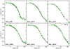 |
Fig. B.1. As in Fig. 3 but for radial density profiles derived by applying a bootstrap sampling. Dashed lines are the best SPES model fits. |
Best-fitting parameters of SPES models using a bootstrap sampling.
Appendix C: Individual model fits
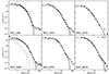 |
Fig. C.2. As in Fig. 3 but with the best LIMEPY Wilson models fits. Grey areas represent 50 randomly selected solutions of the 500 total realisations. |
All Tables
Best SPES models fitting parameters for different membership probabilities thresholds.
All Figures
|
Fig. 1. Gaia EDR3 colour–magnitude diagrams of the studied clusters for stars with high membership probabilities, p ≥ 0.4 (see text for details). The different populations are plotted in different colours: RGB/RC (red), SGB (magenta), TO (green), MS (blue), candidate BSS (cyan squares), and candidate binaries (light grey). |
| In the text | |
|
Fig. 2. Spatial distribution in Cartesian coordinates (x, y) of the studied cluster. The size of the points is proportional to the astrometric membership probability. The different populations are colour coded as in Fig. 1, excluding the binaries and BSSs for clarity. The dark grey arrows in the bottom left corner show the direction of motion and their length is proportional to the velocity in each axis. The light grey arrows in the top right corner show the direction to the Galactic centre. |
| In the text | |
|
Fig. 3. Radial density profiles of the studied clusters. We overplot the best fits of the King (green dashed lines), Wilson (purple dot-dashed lines), LIMEPY (blue solid lines), and SPES (red solid lines) models. |
| In the text | |
|
Fig. 4. Cumulative projected radial distribution of the different populations identified in each of the clusters normalised to the total number of stars in each population. Error bars are not plotted for clarity. |
| In the text | |
|
Fig. 5. rh/RJ (top), rt/RJ (middle), and rt/rc (bottom) as a function of Rgc, Z, τrh, Mcl/Mini, and cluster mass. The clusters studied here are labelled with different colours as a function of age, and are marked with symbols to facilitate their identification. Grey dots are the clusters studied by Angelo et al. (2023). |
| In the text | |
|
Fig. 6. Slope of the outermost region of the radial density profile as a function of the last time the clusters crossed the disc. The clusters are colour coded as a function of their actual distance to the Galactic plane and the same symbols are used as in previous figures. |
| In the text | |
|
Fig. B.1. As in Fig. 3 but for radial density profiles derived by applying a bootstrap sampling. Dashed lines are the best SPES model fits. |
| In the text | |
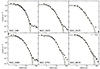 |
Fig. C.1. As in Fig. 3 but with the best LIMEPY King models fits. |
| In the text | |
|
Fig. C.2. As in Fig. 3 but with the best LIMEPY Wilson models fits. Grey areas represent 50 randomly selected solutions of the 500 total realisations. |
| In the text | |
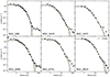 |
Fig. C.3. As in Fig. 3 but with the best LIMEPY models fits. |
| In the text | |
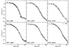 |
Fig. C.4. As in Fig. 3 but with the best SPES models fits. |
| In the text | |
Current usage metrics show cumulative count of Article Views (full-text article views including HTML views, PDF and ePub downloads, according to the available data) and Abstracts Views on Vision4Press platform.
Data correspond to usage on the plateform after 2015. The current usage metrics is available 48-96 hours after online publication and is updated daily on week days.
Initial download of the metrics may take a while.