| Issue |
A&A
Volume 687, July 2024
|
|
|---|---|---|
| Article Number | A146 | |
| Number of page(s) | 17 | |
| Section | Stellar structure and evolution | |
| DOI | https://doi.org/10.1051/0004-6361/202347700 | |
| Published online | 05 July 2024 | |
Entropy-calibrated stellar modeling: Testing and improving the use of prescriptions for the entropy of adiabatic convection⋆
1
Max-Planck-Institut für Sonnensystemforschung, Justus-von-Liebig-Weg 3, 37077 Göttingen, Germany
2
LESIA, Observatoire de Paris, Université PSL, CNRS, Sorbonne Université, Université de Paris, 92195 Meudon, France
e-mail: This email address is being protected from spambots. You need JavaScript enabled to view it.
3
LUPM, Université de Montpellier, CNRS, place Eugène Bataillon, 34095 Montpellier, France
4
Centro de Astrofísica da Universidade do Porto, Rua das Estrelas, 4150-762 Porto, Portugal
5
Institute of Space Sciences (ICE, CSIC), Carrer de Can Magrans S/N, 08193 Cerdanyola del Valles, Spain
6
Institut d’Estudis Espacials de Catalunya (IEEC), Carrer Gran Capita 2, 08034 Barcelona, Spain
7
Max-Planck-Institut für Astronomie, Königstuhl 17, 69117 Heidelberg, Germany
8
Université de Rennes, CNRS, IPR (Institut de Physique de Rennes), UMR 6251, 35000 Rennes, France
9
Institute of Theoretical Physics and Astronomy, Vilnius University, Saulėtekio al. 3, 10257 Vilnius, Lithuania
10
Zentrum für Astronomie der Universität Heidelberg, Landessternwarte, Königstuhl 12, 69117 Heidelberg, Germany
11
Dipartimento di Fisica e Astronomia Augusto Righi, Università degli Studi di Bologna, Via Gobetti 93/2, 40129 Bologna, Italy
12
School of Physics and Astronomy, University of Birmingham, Birmingham B15 2TT, UK
13
Institut für Astrophysik, Georg-August-Universität Göttingen, Friedrich-Hund-Platz 1, 37077 Göttingen, Germany
Received:
10
August
2023
Accepted:
24
February
2024
Abstract
Context. Modeling the convection process is a long-standing problem in stellar physics. To date, all ad hoc models have relied on a free parameter, α, (among others) that has no real physical justification and is therefore poorly constrained. However, a link exists between this free parameter and the entropy of the stellar adiabat. There are existing prescriptions, derived from 3D stellar atmospheric models, that treat entropy as a function of stellar atmospheric parameters (effective temperature, surface gravity, and chemical composition). This can offer sufficient constraints on α through the development of entropy-calibrated models. However, several questions have arisen as these models are increasingly used with respect to which prescription should be used and whether it ought to be used in its original form, along with the impacts of uncertainties on entropy-calibrated models.
Aims. We aim to study the three existing prescriptions in detail and determine which of them demonstrate the most optimal performance and how it should be applied.
Methods. We implemented the entropy-calibration method into the stellar evolution code (Cesam2k20) and performed comparisons with the Sun and the α Cen system. In addition, we used data from the CIFIST grid of 3D atmosphere models to evaluate the accuracy of the prescriptions.
Results. Of the three entropy prescriptions currently available, we determined the one that has the best functional form for reproducing the entropies of the 3D models. However, the coefficients involved in this formulation must not be taken from the original paper because they were calibrated against a flawed set of entropies. We also demonstrate that the entropy obtained from this prescription should be corrected for the evolving chemical composition and for an entropy offset different between various EoS tables. This must be done following a precise procedure to ensure that the classical parameters obtained from the models are not strongly biased. Finally, we provide a data table with entropy of the adiabat of the CIFIST grid, along with the fits for these entropies.
Conclusions. Thanks to a precise examination of entropy-calibrated modeling, we are able to offer our recommendations with respect to which adiabatic entropy prescription to use, how to correct it, and how to implement the method into a stellar evolution code.
Key words: convection / methods: numerical / stars: evolution / stars: fundamental parameters / stars: interiors
Full Table A.1 is available at the CDS via anonymous ftp to cdsarc.cds.unistra.fr (130.79.128.5) or via https://cdsarc.cds.unistra.fr/viz-bin/cat/J/A+A/687/A146
© The Authors 2024
 Open Access article, published by EDP Sciences, under the terms of the Creative Commons Attribution License (https://creativecommons.org/licenses/by/4.0), which permits unrestricted use, distribution, and reproduction in any medium, provided the original work is properly cited.
This article is published in open access under the Subscribe to Open model.
Open access funding provided by Max Planck Society.
1. Introduction
Convection modeling is a major problem in the context of obtaining realistic stellar evolution models. Stellar convective regions are highly turbulent media where the Reynolds number can reach values on the order of 108 (solar photosphere; Komm et al. 1991) to 1014 (bottom of the solar convective envelope; Kupka & Muthsam 2017). In such regimes, Navier-Stokes equations can only be solved numerically. Conducting such hydrodynamic simulations would require high spatial resolutions on a large domain going from the top of adiabatic region to the outer layers of the photosphere and over a timescale of stellar evolution. This is completely unachievable with the computational capabilities available presently and even in the foreseeable future.
To circumvent this problem, physicists have designed ad hoc models that manage to reproduce the general properties of stellar convective envelopes, including their thermal structure. Among them, we can cite: mixing length theory (MLT; Böhm-Vitense 1958) or full spectrum of turbulence models (FST; Canuto & Mazzitelli 1991, 1992; Canuto et al. 1996). The MLT reduces the spectral energy cascade of turbulence to a Dirac distribution, namely: the whole convective flux is carried by eddies of a single size. A hot parcel of matter, before dissolving into the surrounding medium, rises a certain distance (called the mixing length) ℓ = αMLTHp, where Hp is the pressure scale height and αMLT is a free parameter. In deeper regions of the star, convective energy transport is very close to adiabatic, which is isentropic, the thermal structure is then independent of the convection formulation, and (in particular) of αMLT, which is used in the models (Gough & Weiss 1976). However, when the adiabaticity assumption breaks down, typically in low-density near-surface layers in convective stellar envelopes, the value of αMLT determines the degree of non adiabaticity in the model, namely: the entropy difference between the minimum of entropy occurring at the top of the convective envelope and the fully adiabatic interior. The FST represents an attempt to work around this dependence. It assumes a more complex form for the cascade, for instance, a Kolmogorov spectrum. Original formulations of the FST models do not introduce any free parameters and define the mixing length simply as the distance, z, to the nearest boundary of the convective zone. For the purposes of fine-tuning this approach, Canuto et al. (1996) introduced a dependence on the pressure scale height through a free parameter αFST, intended to be small and to experiencing only small changes from a model to another.
However Ludwig et al. (1999) found, using the thermal structures obtained from 2D radiation hydrodynamics (RHD) stellar atmosphere models that αFST does not remain small and varies by a similar amount as αMLT over the HR diagram. Over recent decades, there have been many works highlighting the successes and caveats of MLT and FST models (e.g., Arnett et al. 2015; Trampedach 2010; Kupka & Muthsam 2017) and trying to improve or to go beyond them (e.g., Gough 1977; Grigahcène et al. 2005; Li 2012; Pasetto et al. 2014; Gabriel & Belkacem 2018).
Nonetheless, MLT and FST models remain widely used in stellar evolution codes. The most practical issue these models raise is: how do we choose the value of the free parameter α1? Overall, there are two ways to choose the α value. Firstly, through an optimization process, α can be tuned so that stellar models match a set of observable constraints for one or several stars. The most straightforward case is the widely used solar calibration, in which α is obtained by adjusting its value (together with the chemical composition) of models to reproduce the present-day global solar properties (e.g., Christensen-Dalsgaard 1982; Morel et al. 2000; Serenelli 2016; Vinyoles et al. 2017). The same α value is then used to compute stellar models. This assumes that a unique value of α is appropriate for all stars at all evolutionary stages but there is no reason a priori why this should be the case (Ireland & Browning 2018) and RHD simulations of convective stellar atmospheres consistently point to a variable α (Trampedach et al. 2014; Sonoi et al. 2019). A possible extension would be to use stars, or sets of them, as calibrators, ideally establishing a semi-empirical relation between α values and stellar fundamental parameters. There is, however, a lack of reliable calibrators for which the stellar parameters are known with high enough level of accuracy.
Secondly, a different approach is to consider α as a completely free parameter that can be optimized on star-by-star basis to find best-fitted stellar models to a set of observables. This can be done using either stellar models that are computed as part of the optimization process or pre-computed grids of models with different α-values together with an interpolation algorithm (e.g., SPInS; Lebreton & Reese 2020) to find the best-fit model. This is actually not a calibration, as the resulting α values are not used as the basis for modeling other stars, only to obtain a best-fit model. However, such an approach offers little hope of improving on our formulations and understanding of convection.
To improve the use of MLT or FST modeling of convection, it is necessary to find a relationship between α and global stellar parameters (effective temperature, surface gravity, and chemical composition). This is the aim of α calibrations. Ludwig et al. (1999) used standard 1D stellar atmosphere models with a tunable αMLT parameter (similar to what we have in stellar evolution models) and a grid of more realistic two-dimensional (2D) radiative-hydrodynamics stellar atmosphere models, to find a relation between αMLT, Teff, and log g. More precisely, they adjusted the value of αMLT so that the specific entropy of the adiabat of their envelope models matches the one of their 2D models. This work provided an expression for αMLT as a function of effective temperature, Teff, and surface gravity, g, of the models. Aiming at improving this pioneering study, similar work was carried out by Trampedach et al. (2014) using solar-metallicity 3D atmosphere simulations computed with the Nordlund & Stein (1990) code and later by Magic et al. (2015) with 3D STAGGER models with a metallicity of [Fe/H] ∈ [ − 4.0; +0.5]. More recently, Sonoi et al. (2019) used a grid of 3D stellar atmosphere models computed with CO5BOLD (i.e., COnservative COde for the COmputation of COmpressible COnvection in a BOx of L Dimensions, with L = 2, 3; Freytag et al. 2002, 2012; Wedemeyer et al. 2004) to obtain a representation of α as a function of global stellar parameters for MLT and FST modeling, as well as for different temperatures, T, versus the optical depth τ relations (T(τ) relations) used to describe the atmosphere. All those prescriptions for α are very easy to implement in a stellar evolution code. However, they are highly dependent on the physical ingredients, as it is shown by the important change of calibrated α values introduced by a change of T(τ) relation.
At the same time, Tanner et al. (2016) suggested directly adjusting the α parameter in stellar evolution calculations along the evolution such that the specific entropy of the model adiabat, sad, matches (at all times) sRHD, the value obtained in RHD simulations for the same Teff, log g, and [Fe/H] values (notations for the various specific entropies are summarised in Table 1). This has the advantage that the specific entropy has a well defined physical meaning and is linked to the surface properties of the star by means of the realistic RHD models. In this way, α simply becomes a parameter used to ensure that stellar models reproduce the correct sRHD, as inferred from RHD simulations, in a consistent way with the physical ingredients in the stellar evolution models; for instance, different T(τ) relations, use of MLT or FST, or any other prescription for convection. The idea of Tanner et al. (2016) was implemented in Yale Rotational stellar Evolution Code (YREC; Demarque et al. 2008) and tested on the Sun (Spada et al. 2018) and on the α Cen system (Spada & Demarque 2019). Finally, the method was extended to evolved stars (Spada et al. 2021).
Summary of the different notations used to denote the specific entropy.
The aim of the present work is to contribute to the general effort to develop more accurate stellar models. Modeling the atmosphere of solar-type stars is based on three main components: (1) the opacity profile in the atmosphere, (2) the T(τ) relation which defines the transition in the temperature gradient between optically thick and optically thin regions, and (3) the convection formalism. For a seismically reliable stellar model, these three components must be chosen with the utmost care. This work focuses on the last component by removing the main free parameters of the convection formalism. Specifically, in this work, we built on previous works to produce stellar models that no longer include the mixing length as a free parameter. To that purpose, we implemented the same method in the stellar evolution code Cesam2k20 (formerly known as CESTAM: Code d’Evolution Stellaire avec Transport, Adaptatif et Modulaire; Morel 1997; Morel & Lebreton 2008; Marques et al. 2013), as in the YREC code (Demarque et al. 2008). The previous works made it clear that a lot of care must be taken in the use of entropy prescription. In Sect. 2, we review the available prescriptions and in Sect. 3, we describe the implementation of entropy calibration in Cesam2k20. In Sect. 4 we describe the necessary improvements that should be added to the prescriptions. A discussion is presented in Sect. 5, followed by our conclusions in Sect. 6.
2. Available prescriptions for entropy at the bottom of the convective envelope
2.1. Stellar atmosphere codes
Before describing the entropy prescriptions, it is worth considering a few details on the 3D radiation-hydrodynamics model atmosphere codes that were used to compute the simulations they are based on. The atmosphere codes can solve hydrodynamic and radiative transfer equations. All simulations used hereafter do not include the magnetic field and therefore are referred to as RHD simulations. The codes rely on the “box-in-a-star” setup, where only the flow included in a box is simulated. This box covers an optical depth range of −6 ≤ log10τRoss ≤ 5, which encompasses the superadiabatic region. This domain is small in comparison to stellar dimensions but large enough to resolve properties of the convective flow. Periodic boundary conditions are assumed at the vertical faces of the box and, at horizontal faces, the flow is free to enter and leave the box. The upper boundary condition can vary from one code to the other. At the bottom, the specific entropy of the inflowing material is fixed, which allows for the effective temperature of the resulting model to be constrained. The specific entropy of the inflow can be seen as the entropy of the adiabat. Because at the lower boundary, inflow and outflow do not have the same entropy, the horizontally average at this depth is not equal to the entropy of the adiabat.
In the following, we use spresc to denote the specific entropy obtained from a prescription, sRHD the specific entropy of the adiabat of an atmosphere model, and the word “entropy”, as applied as a synonym for “specific entropy” (entropy per unit of mass). Up to now, three different mathematical formulations have been proposed to relate sRHD to Teff, log g and, optionally, [Fe/H]. While their general mathematical forms remain similar, they have been calibrated on different sets of models.
2.2. The functional form of Ludwig et al. (1999)
The original idea that models of surface convection could be used to derive constraints on the value of the entropy of the adiabat was first suggested by Steffen (1993). Ludwig et al. (1999) (hereafter L99) used a grid of 58 two-dimensional RHD atmosphere models with 4300 K ≤ Teff ≤ 7100 K, 2.54 ≤ log g ≤ 4.74 and a chemical composition close to that of the proto-Sun composition proposed by Grevesse & Sauval (1998) (hereafter GS98), with Y = 0.28 and Z = 0.016. The entropy of the adiabat is expressed as follows:
 (1)
(1)
where  are constants determined using the grid of models,
  and
and  .
.
2.3. The functional form of Magic et al. (2013)
Magic et al. (2013) (hereafter M13) used a grid (the STAGGER-grid) of 217 3D RHD atmosphere models computed with the STAGGER code (Nordlund & Galsgaard 1995), with 4000 K ≤ Teff ≤ 7000 K in steps of 500 K, 1.5 ≤ log g ≤ 5.0 in steps of 0.5, and seven values of metallicity [Fe/H] = +0.5, 0.0, −0.5, −1.0, −2.0, −3.0, −4.0. The solar chemical composition follows the determination of Asplund et al. (2009) (hereafter AGSS09), for the present Sun. M13 suggested that the entropy of the adiabat ought to be to represented by the following function:
 (2)
(2)
and
 (3)
(3)
where the coefficients  are constants, tuned to fit the entropy sRHD of the STAGGER-grid models,
  ,
,  ,
, ![Mathematical equation: $ \widetilde z = \mathrm{[Fe/H]} $](/articles/aa/full_html/2024/07/aa47700-23/aa47700-23-eq10.gif) . We stress that
. We stress that  must be computed with respect to an AGSS09 chemical mixture. If one wants to use another chemical composition of reference, the coefficients in Eq. (2) should be recomputed. The expression proposed by M13 is essentially the same as the one of L99, except that the M13 one takes into account the metallicity.
2.4. The functional form of Tanner et al. (2016)
Based on the same STAGGER-grid, Tanner et al. (2016) proposed a different form to represent sad as a function of Teff, log g and [Fe/H]:
 (4)
(4)
where s0, x0, β, τ0, A and B are constants, calibrated for each sub-set of models with same metallicity;  and
and  .
.
3. Implementation of entropy-calibration in Cesam2k20
3.1. The Cesam2k20 code
The Cesam2k20 code2 implements the same numerical methods as its predecessors (for details, see Morel 1997 for CESAM, Morel & Lebreton 2008 for CESAM2k, and Marques et al. 2013 for CESTAM). The stellar structure equations are solved using a collocation method where solutions are represented as a linear combination of piecewise polynomials, projected over a B-Spline basis.
Cesam2k20 uses opacity tables either from the OPAL team (Rogers & Iglesias 1992; Iglesias & Rogers 1996) or OP tables from the Opacity Project (Seaton et al. 1994; Badnell et al. 2005; Seaton 2005, 2007). Several equations of state (EoS) are implemented and this work uses tables from the OPAL5 EoS (Rogers & Nayfonov 2002). Concerning the nuclear reaction rates, we used compilations from NACRE (Aikawa et al. 2006) (except LUNA – Broggini et al. 2018 – for the 14N(p, γ)15O reaction).
Regarding the mixing processes, rotation is neglected throughout this work. The effects of atomic diffusion are modeled with the formalism proposed by Michaud & Proffitt (1993). The convection is modeled with mixing-length theory formalism under the formulation of Henyey et al. (1965) taking into account the optical thickness of the convective bubble. We stress that the entropy-calibration method also works with more complex formalisms, such as the one developed by Canuto & Mazzitelli (1991) or by Canuto et al. (1996), assuming a Kolmogorov spectrum for the turbulent convective flow.
A schematic flowchart of steps followed by Cesam2k20 during the computation of a time step is represented in Fig. 1. At a given time step, Cesam2k20 iterates following a Newton-Raphson scheme to find the solution to the structure equations. More precisely, using the stellar structure determined at the previous time step, Cesam2k20 starts by finding the boundaries of the convective zones (CZ), then it evolves the chemical composition to the current time-step, then finally solving the stellar structure for that time. After each iteration, numerical convergence is assessed. If it is satisfied, the solution is accepted and new time step is computed. In general, this process is repeated several times to find an acceptable solution.
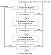 |
Fig. 1. Schematic representation of the step of a Newton-Raphson scheme followed by Cesam2k20 during the computation over a time step. The “problem” can be an unconverged solution, an interpolation outside EoS, or opacity table. |
3.2. Scheme for entropy-calibration
As mentioned in the introduction, the value of αMLT controls the adiabat of the convective envelope of the stellar model. This is easily seen in Fig. 2, where we present an average specific entropy profile extracted from a 3D atmosphere simulation and entropy profiles computed from 1D stellar structures. Despite the fact that 3D and 1D models give very different entropy profiles in the superadiabatic layers, they can converge in deeper layers to the same adiabat, providing we find the correct value of αMLT.
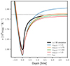 |
Fig. 2. Profile of specific entropy as a function of the depth in the model. The origin of the depth is taken as the location of then entropy minimum in the superadiabatic region. Average specific entropy profile of a 3D simulation is represented as a solid black line, and the entropy of the adiabat as a dash black line. The entropy of the adiabat is an input of the 3D model. Other curves are profiles of specific entropy obtained with 1D models computed with different values of αMLT = 1.5 (blue), 1.75 (orange), 1.82 (green), and 1.9 (red). |
The procedure of entropy calibrations requires an intermediate step between the computation of the new chemical composition and the resolution of the structure equations. This intermediate step is part of the Newton-Raphson iteration described in Eq. (1). In that step, we compute a preliminary version of the entropy sad, 1 and the mean molecular weight (the reasoning is discussed in Sect. 4.2) at the bottom of the convective envelope. These quantities are computed in an approximate stellar structure obtained with a given α1 ≡ α, either from a previous time step or from a previous structure iteration. With the values of Teff, log g and [Fe/H] for this intermediate model, we evaluate the chosen functional representation of sad that provides the entropy spresc, 1 of the adiabat that this model ought to have.
Then, the value of α1 is modified by a small amount: α2 = α1 + δα (currently, δα = 0.001α1). With α2, we call again the routine that solves for the stellar structure. Again, we compute sad, 2 at the bottom of CZ, and the value spresc, 2 that it must take according to the chosen functional. We want to find the correction Δα applied to α1, such that at next iteration we have:
 (5)
(5)
with δsi = (spresc, i − sad, i), i = 1, 2. Then, Δα is:
 (6)
(6)
In the Cesam2k20 input file, the fitting function proposed respectively by Ludwig et al. (1999), Magic et al. (2013), and Tanner et al. (2016) can be set through the option nom_alpha respectively equal to ‘entropy_ludwig99’, ‘entropy_magic13’, and ‘entropy_tanner16’.
3.3. Control of precision and performance
The agreement between sad and spresc is controlled before the end of a time step. If the absolute value of the difference between the two exceeds 105 erg g−1 K−1, the solution is rejected and the computation of the current evolution step is started over again with a time step divided by two. This threshold was found by trial and error, and can be adjusted by the user. To give a comparison, in the STAGGER grid, the total variation of the entropy of the adiabat spans 1.6903 × 10⁹ erg g−1 K−1. Therefore, the criterion is almost always met at the first try and the time step rarely needs to be decreased.
In terms of performance, the use of entropy calibration significantly increases the computation time (by a factor 2 to 3). This is due to the fact that in order to evaluate the effect of a change of α on sad, one has to recompute the entire stellar structure with α + δα. YREC proceeds differently: the envelope and the rest of the star can be computed separately and this can provide the new adiabat sad, 2 much faster. In Cesam2k20, the interior and the envelope are solved together and the calculation cannot be decoupled.
4. Amendments to the entropy prescription
4.1. A first naive implementation
Once the entropy calibration procedure has been implemented into Cesam2k20, the next question is how the method impacts a standard3 evolutionary track. To do so, we first calibrated a standard solar model (SSM) with a chemical composition following the determination of GS98 which is close to the one used in the 2D atmosphere grid that the L99 function was fitted on. The opacity and EoS are interpolated from the OPAL5 tables, convection is treated in the MLT framework, gravitational settling is modeled using the Michaud & Proffitt (1993) approximation and no rotation is assumed. The atmosphere is reproduced using the reduced T(τ) relation, known as the Hopf function, q(τ):
![Mathematical equation: $$ \begin{aligned} T(\tau ) = T_{\rm eff} \left[ \frac{3}{4}\left(q(\tau ) + \tau \right)\right] ^{1/4}. \end{aligned} $$](/articles/aa/full_html/2024/07/aa47700-23/aa47700-23-eq17.gif) (7)
(7)
The Eddington T(τ) turns into a constant q(τ) = 2/3. Other choices are discusses in Sect. 5.1.3.
This SSM is calibrated by adjusting the initial helium mass fraction Y0, initial metal to hydrogen ratio (Z/X)0 content, and the parameter αMLT to match (at a solar age) the luminosity, 1 L⊙ (L⊙ = 3.828 × 1033 erg s−1 cm−2; Mamajek et al. 2015), the effective temperature 5772 K, and the current surface (Z/X)s of the Sun with a maximum error of respectively 10−5, 1 K and 10−5. These parameters are adjusted using a Levenberg-Marquardt algorithm implemented in the Optimal Stellar Model program (OSM4; for detailed applications, see Castro et al. 2021). This package is currently interfaced with the Cesam2k20 code and finds the model that best matches a set of observational constrains (in that sense, it can be considered an “optimal” model). Best values found for adjustable parameters of the model are reproduced in Table 2. Once this optimal model has been obtained, we recompute the evolution by keeping everything identical, except that this time, the value of αMLT is adjusted at each time step during its evolution to match the entropy prescribed by either L99, M13 or T16. These models are called entropy-calibrated models (ECMs).
Parameters of the SSM model.
The resulting evolutionary tracks are represented in Fig. 3, left panel. As can be seen, the four models follow very different paths. During the PMS, the locations of the respective Hayashi tracks are very far apart, while all models follow quite a similar Henyey track (Henyey et al. 1955). At a solar age, the shift in effective temperature can reach ≃130 K, with respect to the SSM. Models computed with M13 and T16 lead to similar results for evolved phases after the terminal age main sequence (TAMS), but they significantly differ from the one obtained with L99.
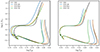 |
Fig. 3. HR diagram of a standard solar model (black line) and associated entropy-calibrated models shown in the left panel, with the uncorrected prescriptions: L99 (blue), M13 (orange), and T16 (green) taken “as is” Dots represent the location of each model at solar age. Right panel displays the HR diagram of a standard solar model (black line) and associated entropy-calibrated models with the prescriptions L99 (blue), M13 (orange), and T16 (green) corrected using Eq. (11). Dots represent the location of each model at solar age. |
We see that ECMs are different from SSM, but are they better? The discrepancies obtained at a solar age are problematic: the Sun must have a definite entropy for its adiabat, however, all prescriptions give very different values for the same set of input values. With this first implementation, it would seem that entropy-calibration is not very robust for stellar models. Moreover, the shift observed on the RGB between the track computed with L99 on the one hand, and the tracks computed with M13 and T16 (on the other hand) may reveal large differences between the grids on which these functions are adjusted. These issues stress the fact that the prescriptions should not be used at face value (as given in the original papers), but at least corrected.
4.2. On the proper use of entropy prescriptions
In their works, Spada et al. (2018) and Spada & Demarque (2019) used the entropy given by T16’s mathematical formulation corrected by an offset, ds. Indeed, the entropy is formally defined up to a constant. This constant can differ from one code to another because different EoS tables were used to generate either the atmosphere or the evolution models. Actually, entropies used in the STAGGER-grid to calibrate the coefficients in M13 or T16’s functions were already defined using a constant offset to make possible their comparison to those in the L99 models (see Magic et al. 2013, p. 9).
To compute the offset ds that should be added to spresc, we first need to compute a model with a standard (i.e., a fixed α) and then compare its adiabat to the one predicted by the chosen prescription. Of course, the standard model should use the same physics, and especially the same EoS, as the entropy calibrated model that will be computed.
The second effect that needs to be taken into account is the entropy variation due to a change of chemical composition. Strictly speaking, to conduct entropy calibration, we should always consider models with a chemical composition identical to the one used to fit the coefficients of the entropy representation. However, the chemical composition changes through the star’s life and this should be accounted for. In an ideal gas, neglecting the radiation pressure and assuming a polytropic EoS, one can write the entropy as (e.g., Ireland & Browning 2018):
 (8)
(8)
where s0 is a constant, μ is the mean molecular weight, T the temperature, ρ the density, and γ the adiabatic exponent. A change of chemical composition has its main impact through the mean molecular weight. Because the term s0 in Eq. (8) is small compared to the second term5, the entropy of a given atmosphere model with a mean molecular weight changing from μRHD to μ can be approximated as
 (9)
(9)
This relation is valid only for a small change of μ.
This correcting factor was used in Spada et al. (2021) to account for significant chemical changes in evolved stellar phases but the offset correction, ds, was not used. We recommend, however, using both corrections. So, the next issue is to find out what form the correction should take. Coming back to the computation of the offset, ds, if the standard 1D model and the atmosphere model grid do not share the same chemical composition, then the offset simply computed as ds = sad − spresc does not only depend on a different choice of constant, but also on the different chemical mixtures. Instead, the offset should be adjusted as follows:
![Mathematical equation: $$ \begin{aligned} \mathrm{d} s^\mathrm{presc} = {s_{\rm ad}}^\mathrm{std} - s_{\rm presc}(T_{\rm eff}^\mathrm{std}, \log g^\mathrm{std}, \mathrm{[Fe/H]}^\mathrm{std}) f_\mu ^\mathrm{std}, \end{aligned} $$](/articles/aa/full_html/2024/07/aa47700-23/aa47700-23-eq20.gif) (10)
(10)
where “std” stands for quantities of the standard model,  from Eq. (9) accounts for the change in mean molecular weight, from the entropy prescription (based on 3D RHD simulations) to the 1D standard model we want to apply it to. Then, the corrected entropy takes the form:
 (11)
(11)
This correction is applied every time a prescription is evaluated because fμ changes over the course of the evolution, for instance, as a result of gravitational settling or dredge up.
In order to see the impact of this correction on the evolutionary tracks, we repeated the experiment of Sect. 4.1 but this time the ECMs follow the corrected prescriptions. To compute the entropy offset of each entropy representation, we used SSM as our standard model. The values are given in the first line of Table 3. The evolutionary tracks of SSM and the new ECMs are presented in Fig. 3. Now, we find that all four tracks intersect at solar age. However differences remain during the Hayashi tracks and on the RGB. The Hayashi track is a very short period of time (≃6 Myrs for the Sun), and its modeling is subject to a lot of uncertainties (e.g., Zwintz & Steindl 2022). The differences seen in this phase do not propagate to later evolutionary phases and do not affect the validity of the method. The differences for PMS and RGB models have two sources. First of all, these two regions correspond to locations where the three entropy functional representations have the higher inaccuracies, i.e. largest errors between fitting function and entropy of the adiabat coming from 3D models. Moreover, the entropy of the adiabat does not vary linearly with Teff and log g. The entropy fitting functions of Eqs. (1), (2), or (4), together with coefficients given in Appendix B, show that the entropy of the adiabat increases towards higher Teff and lower log g, but with decreasing slopes in the same direction. Therefore, a given uncertainty on the entropy coming from the fitting procedure, will imply a smaller change of location when the model is on the RGB region than when it is in the PMS. This explains why the discrepancies in the RGB region are smaller than around the Hayashi track. Still, some work remains to be done to improve the method in these evolutionary phases, for instance, by improving the analytic prescriptions in these regions of the Kiel diagram.
Entropy offset ds [109 erg g−1 K−1] computed with the SSM model and for various prescriptions.
4.3. Recommendations on the use of prescriptions
In addition to the a posteriori correction of the prescribed entropy values, the 3D RHD simulation basis for the three formulations (L99, M13, and T16, i.e., a re-fit of M13) are not equivalent. The models used to calibrate the L99 law have been computed in 2D; therefore they may not be reliable enough to reproduce the entropy stratification of 3D models. Furthermore, this relation was obtained only for one (solar) metallicity. Therefore, the correction fμ may not be valid because the difference between μRHD and μ from the entropy calibrated model may not be close enough to zero. For these reasons, we recommend not to use the L99 prescription (with any set of coefficients), except when computing non diffusive models, with a chemical composition similar to GS98. L99 is therefore not used in the remainder of this work.
Regarding the functional forms suggested by M13 and T16, it appears that they have not been originally calibrated against the “true” entropies of the adiabat of the STAGGER grid (i.e., the inputs of the models), but against sbot the average entropy at the bottom of the simulation domain (sRHD values are not publicly available). These simulations assume that at the bottom of the boxes, the adiabat is reached and sbot = sRHD. However, this is only true for some models (see Table A.1) and it introduces significant disagreements between sRHD and the value given by the prescription. On the contrary, in CO5BOLD models of the CIFIST grid, the true entropy of the adiabat is known exactly because it is an input of the simulation and corresponds to the entropy of the inflow at the bottom boundary of the simulation domain. This also mean that the value of sRHD is not flawed by any boundary effect, which is not the case for the value of sbot.
In order to perform a comparison of the various entropy representations (see Sect. 2) and to improve the quality of the entropy calibration, we re-calibrated the coefficients on a set of entropies of the adiabats obtained from 102 models of the CIFIST grid (Ludwig et al. 2009) computed with the CO5BOLD code (Freytag et al. 2002, 2012; Wedemeyer et al. 2004). Here, we use the true entropy of the adiabats, sRHD (and not the one computed at the bottom of the simulated box). These data are available in Appendix A for models with solar metallicity and the coefficients of the functional forms are available in Appendix B. Figure 4 illustrates the impact of re-calibrating the M13 function, defined in Eq. (2). The left column shows  , namely, the entropy difference between the true entropy of the adiabat in the CIFIST grid and the original M13 formulation (“original” in the sense that the coefficients are taken from Magic et al. 2013). We note here that a constant has been added to the original M13 relation to compensate for the zero point offset between the entropy of the solar models in the CIFIST and STAGGER grids, as stated in Fig. 4 caption. The right column in Fig. 4 shows the differences
  , in which
  is obtained after the M13 formulation has been re-calibrated in the CIFIST grid.
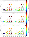 |
Fig. 4. Specific entropy differences in the adiabat Δspresc ≡ sRHD − spresc between values provided by the CIFIST grid (Ludwig et al. 2009), and values predicted by the M13 prescription, Eq. (2). Left column: original coefficients from Magic et al. (2013) are used. Here, entropy from the CIFIST grid has been corrected by an offset of 0.04794 × 10⁹ erg g−1 K−1 corresponding to the entropy difference between the solar atmosphere models in the CIFIST and STAGGER grids. Right column: same as left column but the coefficients involved in the M13 mathematical form have been re-calibrated with the CIFIST entropies. Rows: each row displays the models with a given metallicity: [Fe/H] = +0.0 (row 1), −1.0 (row 2) and −2.0 (row 3). |
The distribution of Δspresc for CIFIST models is also represented as a histogram in Fig. 5. We see that this new calibration reduces the range of entropy differences (from ≃0.05 to ≃0.03 × 10⁹ erg g−1 K−1) but the accuracy of M13 remains similar for the two grids. However, variations of Δspresc across the Kiel diagram do not behave the same. In Fig. 4, left column, the entropy difference rises with decreasing Teff, but in the right column, the larger differences are localized in the PMS region and around the RGB of stars more massive than the Sun. Those differences may arise from two effects: (1) the offset we added does not fully correct the discrepancies between the different EoS and reference solar composition (i.e., these differences do not induce a constant change across the Kiel diagram) and (2) in Fig. 4, left column, coefficients of Eq. (2) are calibrated on sbot instead of spresc.
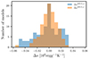 |
Fig. 5. Histogram showing the distribution of the entropy errors Δspresc for the M13 prescription. The data plotted are the same as shown in Fig. 4, for all metallicities. In blue is shown the ΔsM13, o distribution corresponding to differences |

The distributions of Δspresc for the re-calibrated M13 and T16 formulations (Eq. (4)) are represented in Fig. 6. Both prescriptions hardly exceed an absolute error of 0.05 × 10⁹ erg g−1 K−1, which is less than 3% of the extremal variation of entropy across the CIFIST grid. This agreement is very satisfying. In addition, we note that the distribution of ΔsM13, r is much more peaked around 0.0 than the one of ΔsT16, r. This comparison advocates for generalizing the use of the M13 prescription in entropy-calibrated modeling. From this point onwards, we only use the M13 prescription of adiabatic entropy.
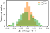 |
Fig. 6. Histogram showing the distribution of the entropy errors between sRHD and spresc for M13 and T16 entropy representations. Both functions have been re-calibrated on entropies from the CIFIST grid. |
5. Discussion
5.1. Possible sources of uncertainties
The accuracy of entropy calibration modeling can be affected by several factors. In the following section, we review them and estimate their impact on the determination of a star’s characteristics. One source of uncertainty is the already mentioned gap between sRHD and the corresponding value obtained from prescriptions. Accuracy can also be impacted by the methods used to determine the offset ds, along with the sad and μ values at the bottom of the convective envelope of the stellar evolution model. Then, we should also examine what happens when a prescription is evaluated outside of its domain of definition. Finally, it could be expected that a different choice of T(τ) relation would change the location of an evolutionary track on the HRD or Kiel diagrams. These points are investigated in the following subsections.
5.1.1. Determination of μ and sad in 1D models
Several factors can affect the accuracy of entropy-calibration modeling. The first one comes from the way we determine the mean molecular weight μ (in order to compute fμ) and the entropy of the adiabat in the 1D model.
The mean molecular weight depends on the relative abundance and on the ionization rates of each element. Strictly speaking, the mean molecular weights in the 3D simulations and in the 1D models should be compared assuming well-defined ionization states between the two chemical compositions. The proper way to compute μ1/3D would be to use the same EoS in the 1D and 3D code, and evaluate them for a given state (given pressure, temperature and chemical composition). However, we want to be able to use any EoS in the 1D code, possibly different from the one used in the 3D simulations. Moreover, not only is the chemical composition different in the 1D and 3D simulations, but also the elements considered are not the same. To get around these issues, we can assume that at the bottom of the convective zone, the material is fully ionized. This is not exactly true, but it has the merit of considering the same ionization state for the two mixtures. In this case, μ can be approximated as μ−1 = 2X + 3Y/4 + Z/2 where X, Y an Z are respectively the hydrogen, helium and metal abundance. The error on fμ induced by this approximation is below 1% for stars with M < 1.5M⊙. We could relax this approximation by assuming that the ionization rates are the same in the evolutionary and in the atmosphere models. This would allow us to consider each element individually, instead of a dependence in X, Y, and Z. However, for this to work, it would require us to consider exactly the same chemical elements in both simulations, which would involve too much constraint from a modeling point of view. In any case, this would modify the value of μ by an almost constant factor, which would be taken into account in fμ, as defined in Eq. (9).
With respect to the determination of the entropy of the adiabat in the 1D model, we compared the three available methods. In the first one, we defined  as the value of the entropy exactly at the transition between the radiative zone and the convective envelope. Another method would be to define
  as the average of the entropy in a sub-region of the adiabatic region. This second method would require us to interpolate in the EoS table for each layer in the sub-region, which is time-consuming. To improve its efficiency, we introduce instead a third definition, whereby
  is the average of the entropy computed for every ten layers in the sub-region only.
Figure 7 represents the entropy profile in the adiabatic region of SSM. We stress that the figure is extremely zoomed-in and what seems to be large fluctuations is actually nearly constant. Starting from T ≃ 105 [K] to the right, we see a decrease of entropy, corresponding to the beginning of the superadiabatic region. The value of  is represented as the blue line. The green shaded area corresponds to the sub-regions where
  and
and  have been defined. The green region represents 10% of the radial extension of the convective envelope and ≃66% of its total mass. This extent is chosen arbitrarily but ensures that, for every model in the domain of definition of the CIFIST grid, we only enclose a sub-region of the adiabatic region. Clearly,
  and
and  are nearly equal. So, we consider why the use of
  instead of
  would give significantly different results and discuss these possibilities below.
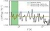 |
Fig. 7. Entropy as a function of temperature (black line) in a sub-region of the convective envelope of SSM. The value of entropy at the limit between radiative and convective zone is represented as a blue line. The average of entropy in the green shaded area is represented as a green line and the average of entropy at orange points is represented as a dashed orange line. The green area has a width of 10% of the total width of the CZ (roughly |

We implemented both definitions in Cesam2k20 and computed two evolutionary tracks using the M13 prescription. Tracks are shown in a HR diagram in Fig. 8. In terms of global quantities, the two definitions give similar results. However, as stressed by the subplot showing a zoom of the Hayashi track, using  gives a more irregular path than
  , whereas using
  actually significantly increases the numerical stability of the method.
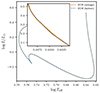 |
Fig. 8. HR diagram of the same entropy-calibrated model, using the M13 prescription, but different methods for evaluating the entropy of the adiabat in the 1D structure model: |


5.1.2. Constancy of the entropy offset, ds
The way we computed the offset, ds, immediately brings on the concern that it may vary across HR diagram. As said before, the offset ds corrects for a systematic difference in the entropy of the 3D atmosphere grid and the one computed in the stellar evolution model. This offset is the sum of the entropy zero-point for that EoS, and an ad-hoc constant for it to match the L99 entropy. The offset should be estimated with a standard solar model (standard in the sense that αMLT stays fixed along evolution), which provides us with the most accurate constraint one can obtain on the entropy of the adiabat.
In order to verify that ds is almost constant over the HR diagram, we computed entropy for three different EoS (numerical or analytical), for a given chemical composition, and conditions of pressure and temperature that cover the ones found at the bottom of convective envelope of stellar models with a mass between 0.8 to 1.3 M⊙. The three EoS are the OPAL5 equation of state, the simple EoS proposed by Wolf (1983, hereafter noted as W836) and FreeEOS (Irwin 2012). OPAL5 is the EoS table used to compute Cesam2k20 models. The simple analytic EoS proposed by W83 is the one used by CO5BOLD. Here, we implemented a simplified version which accounts only for H+, He+, He++, e− and a representative metal (case f. in W83). FreeEOS is also an analytic EoS but much more detailed. We followed FreeEOS’s recommendation and adopted the version suitable for stellar interiors that also reproduces the MHD equation of state (Mihalas et al. 1988) used by the STAGGER code. This version includes 20 elements with 295 ionization states. The entropy differences between FreeEOS (resp. W83) and OPAL5 are presented in a log10p − log10T plane in left (resp. right) panel of Fig. 9. Extremal variation in this interval is on the order of 107 erg g−1 K−1. This is negligible compared to, for instance, the extremal variation of entropy across the CIFIST grid (1.69 × 10⁹ erg g−1 K−1). In addition, these extremal variations are reduced if we exclude top left (resp. bottom-right) corner that corresponds to regions of low p – high T (resp. high p – low T), which are never found at the bottom of the convective envelope of our models. Therefore, the assumption that offset, ds, is constant over the HR diagram holds to good accuracy.
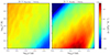 |
Fig. 9. Entropy differences between two EoS, in the log10p − log10T plane. The colour codes for the entropy difference. Left panel: entropy differences between free EOS and OPAL5. Right panel: entropy differences between EoS of Wolf (1983) and OPAL5. |
5.1.3. Impact of the T(τ) relation
The previous attempts to prescribe a value for αMLT have in common the weakness that the α prescription depends on the kind of T(τ) relation chosen to reproduce the atmosphere. This issue disappears with entropy calibration modeling, as shown in Spada et al. (2018) for the Sun and in Spada et al. (2021) for MS and RGB stars. The reason is that the entropy of the adiabat depends on the characteristics of the adiabatic layers, not on how the atmosphere is computed. The adiabat of the convective envelope of a star depends solely on the star’s location in the Kiel diagram and its metallicity. If the T(τ) relation changes, the value of αMLT will adapt, but the location on the Kiel diagram is the same. To verify that this property remains true with our procedure, we computed four identical solar entropy calibrated models except for the T(τ) relation that follows either an Eddington law, a fit of Vernazza et al. (1981)’s Model C of the quiet Sun, the Krishna Swamy (1966) relation, or a T(τ) relation recently proposed by Ball (2021).
A change in the T(τ) relation, at a fixed αMLT, changes global quantities such as Teff. However, here, we are adjusting αMLT to match a given entropy of the adiabat, therefore changing the T(τ) relation does not imply a change of location in the HR diagram. In the top panels of Fig. 10, we represent the evolution with age, starting from PMS, of the relative L, R, Teff and the absolute sad differences for models computed with various T(τ) relations, with respect to a standard model computed with the Eddington T(τ) relation. It clearly shows the invariance of such global quantities when a different T(τ) law is chosen. On the bottom left panel, we show αMLT along evolution for the same models. Since, Teff, log g and the metallicity are the same from one model to the other, sad also remains constant. The structure of superadiabatic layers at final age (4570 Myrs) is shown in the bottom panel of Fig. 10. It stresses that T(τ) relations have an important impact on the modeling of the shallowest layers but the structures are all identical when deep enough in the star. The deepest layer shown in the figure has a pressure of 107 dyn cm−2, which is well above the bottom of the convective envelope, located around a pressure of 1013 dyn cm−2. It highlights the fact that although the choice of T(τ) relation does not impact global properties of the model, this choice is still crucial for obtaining realistic models for asteroseismology.
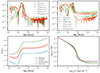 |
Fig. 10. Comparison of luminosity (solid lines) and effective temperature (dashed lines) for four models computed with different choices of T(τ) relation (top-left). The displayed quantity is the relative difference of L or Teff, with respect to model computed with the Eddington T(τ) relation: δX ≡ (XT(τ) − XEdding.)/XEdding.. Top right panel is the same as top left panel but, instead of X ≡ sad, we display the absolute difference. Indeed, with sad being defined up to a constant, the relative difference would have no meaning. Also, Δspresc is in the units: 109 erg g−1 K−1. Bottom left panel: evolution of αMLT for different T(τ) relations: Eddington (blue), Vernazza et al. (1981) Model-C (orange), Krishna Swamy (1966) (green), and Ball (2021) (red). Bottom right panel: temperature as a function of the pressure for the same four final models at solar age. |
The examination of the bottom left panel of Fig. 10, reveals a minimum in the αMLT variation with age between 2 and 6 Myrs, when models are on their Hayashi track. It is not possible to relate this behavior to previous calibrations of αMLT of Ludwig et al. (1999) or Magic et al. (2015), but only with the one of Trampedach et al. (2014) or Sonoi et al. (2019) for what they called “Eddington + MLT(BV)”. This last work calibrated αMLT by matching 1D CESTAM structure models to 3D CIFIST atmosphere models. CESTAM (and also its successor Cesam2k20) implements two versions of the MLT that assume either a linear temperature distribution in the convective bubble (that Sonoi et al. 2019 called “BV”) or a distribution that obeys a diffusion equation, as suggested by Henyey et al. (1965). The BV version of MLT is also the version used in the work of Trampedach et al. (2014) and in this work, which explains the agreement.
5.1.4. Interpolation outside the prescription’s domain of definition
It may happen that at some stage of the evolution, a model falls outside the domain of definition of the prescription, which is the domain covered by the CIFIST grid in this work. For instance, when starting from the PMS, a solar model spends its first 1 Myrs slightly outside this domain.
Every time a given prescription is evaluated, Cesam2k20 checks if the model (its (Teff, log g, [Fe/H])) is inside the convex hull of the set of 3D models. By default, Cesam2k20 only sends a warning (this behavior can be changed by the user), and proceeds to evaluate the prescription. It must be noted that if prescriptions are evaluated outside of the domain, on the hot side, the resulting entropy can diverge because of the positive term in the exponential of Eqs. (1) and (2)). On the cool side, the exponential should remain small and the entropy does not diverge (which does not mean its value is reliable). The only solution to circumvent this issue is to extend the range of definition of the prescriptions. This work is currently in progress.
5.2. Comparison with YREC: The α Cen system
As a final test, we compared the results of modeling the α Cen system computed with standard or entropy-calibrated modeling, to the models presented in Spada & Demarque (2019, hereafter SD19). The microphysics of the models is kept as close as possible to the one used in YREC models: the MLT treatment of convection, Eddington atmosphere, and element abundance ratios following the GS98 chemical composition and only gravitational settling is taken into account in the diffusive treatment. SD19 used the YREC code to obtain best fitting models of α Cen A and B, using a Markov chain Monte Carlo (MCMC) method (more details given in SD19). The use of the MCMC method allowed the authors to provide reliable uncertainties to their best estimated parameters. To speed up the process, evolution models were started at the ZAMS.
In the present work, we found optimal Cesam2k20 models for the α Cen system using the OSM program. In our calibrations, we used the same observational constraints as the one used by SD19, summarized in Table 4 and we adjusted the age of the model, its initial helium content Y0, its initial (Z/X)0 ratio and (only for the standard models) the αMLT, so that we match the observed radius, luminosity, and current (Z/X)s. In ECMs, of course, αMLT is varying along evolution, following the change of entropy. The mass is not a free parameter: we used the value reported in Table 4. In parallel, using the same physical ingredients, we calibrated a solar model to be the standard model for the computation of entropy offset ds. Using the M13 prescription yields ds = 0.0264 × 10⁹ erg g−1 K−1 and we used this value to compute entropy-calibrated models by tuning the same parameters as before (except for αMLT). The Levenberg-Marquardt scheme implemented in OSM cannot yield reliable uncertainties and therefore, we give our best estimated parameters, without uncertainties. The squared-distance χ2 between the best Cesam2k20 model and the observational constraints is computed with:
 (12)
(12)
Observable constraints and optimal parameters derived for the α Cen system.
where  are the observational constraints, σi their uncertainties, and
  are the values of the same parameters in the best model. The MCMC method used by SD19 explores a wide parameter space, and then requires the computation of more models than OSM. Therefore, we could afford to start our Cesam2k20 models from the PMS.
The optimal parameters obtained with YREC and Cesam2k20 are presented in Table 4. Top panels of Fig. 11 show the tracks of all models in the radius − luminosity plane with the measured location of α Cen A and B. Models taken from SD19 show slightly worse agreement with observational constraints than models computed for the present work. This is only a consequence of the optimization scheme: since the MCMC method explores all the parameter space, a very large number of models need to be computed and obtaining a very precise solution is extremely time consuming. Alternatively, OSM requires to compute only a small number of models and the optimal solution is guided to a (possibly local) minimum.
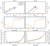 |
Fig. 11. Evolutionary tracks (top) for α Cen A (left panel) and α Cen B (right panel) on the R − L plane. Tracks computed in the present work are represented as solid lines, while the one from Spada & Demarque (2019) are drawn as dashed lines. Standard models are in blue and EC models in orange. Evolution of αMLT as a function of age (middle) for the same models. Evolution of the convective envelope depth (bottom) along the evolution. |
The differences obtained between YREC and Cesam2k20 models can have a number of causes. First of all, the numerical schemes differ. The convective envelope is treated separately from the core in YREC, which allows it to tune α by recomputing only the envelope structure. This is not possible with Cesam2k20 and we have to recompute the complete structure every time α is changed. Also, in the case of ECM models, different entropy prescriptions are used and the way of correcting them differs. SD19 also made use of the T16 function with the coefficients taken from the original paper while we used the M13 function with coefficients re-calibrated on the CIFIST grid. In addition, it must be stressed that the model of α Cen B has its Hayashi track outside the domain of definition of M13, which was not the case for models in SD19, because their tracks started from the ZAMS. However, it represents a very short time of the life of α Cen B and should not have significantly impacted its evolution. Finally, SD19 corrected the prescribed entropy using only the entropy offset while Cesam2k20 also corrected for differences in the chemical composition. These discrepancies translate in quite different evolution of αMLT between models with similar physics. However, the general trend remains similar: αMLT increases when sad increases. The variations of entropy can easily be understood with the approximation that  . With the virial theorem, it follows that T ∝ R−1 and ρ ∝ R−3, with R being the total radius of the star. Therefore, during expansion phases, when R increases, sad increases, and the inverse is true during the contraction phases.
The bottom panels of Fig. 11 display the variation of the depth of the convective envelope dcz for all models of the α Cen system. Once again, it reveals a very good agreement between YREC and Cesam2k20 models. Whereas αMLT depends a lot on the physical ingredients and numerical methods used in the code and does not have a precise physical meaning, dcz is a measurable quantity. Having such an agreement for dcz between the two codes advocates for the reliability of the method. Moreover, the values of dcz predicted for a standard and EC models are close, but not identical. For α Cen B (the less massive), the two values are almost equal during the main sequence, while in the case of α Cen A (the more massive), the ECM predicts a shallower CZ at the ZAMS and deeper at the present age of α Cen A. If confirmed, such pattern should have repercussions on the transport of chemicals and angular momentum.
6. Conclusion
In this work, we present a comprehensive description of the entropy-calibrated modeling, along with details on how to properly implement and apply it. The entropy-calibration consists in adjusting the value of the convection parameter, α, so that the entropy of the adiabat in a stellar structure model matches the one predicted by an entropy prescription.
We studied and compared the accuracy of the three available prescriptions for the entropy of the adiabat suggested in Ludwig et al. (1999), Magic et al. (2013) and Tanner et al. (2016). Those functions are adjusted to fit the entropy of the adiabat in stellar atmosphere simulations, as a function of Teff, log g, and [Fe/H] in a grid of such simulations. Our study points out the fact that the M13 fit was based on the entropy, averaged over both the adiabatic up-flows and the cooled down-flows, at the bottom boundary of their RHD simulations – instead of on the entropy of the asymptotic adiabat. T16 is a refitting of those same, flawed entropies, introducing a bias on the prescribed entropy value. After the re-calibration of the entropy functional representations using the correct set of entropies of the adiabat obtained from the CIFIST grid (Ludwig et al. 2009), we show that the functional form that most accurately reproduces the RHD results and, therefore, the one we recommend is the formulation proposed by Magic et al. (2013) with coefficients given in Table B.2. We have made the quantities extracted from the CIFIST grid that have been used in this work publicly available. The coefficients of the fitting functions are also given in Appendix B, which extends the small list of entropy prescriptions available to the stellar modeling community.
We note that not only must the prescription be carefully chosen, but its use must be correctly set up. Spada et al. (2018) first proposed to correct the prescribed entropy with an offset that corresponds to a different choice of entropy integration constant between different EoS tables. In contrast, Spada et al. (2021) proposed to only correct the prescription for the influence of a different chemical composition between the one used in the evolution and in the atmosphere model. We demonstrate in this work that both corrections must be used. In order to compute entropy-calibrated models, the steps are as follows:
-
Compute a standard (i.e. not with entropy-calibration) model of reference. We advocate using a solar model as the reference because it is the star with the best observational constraints available. This standard model must implement exactly the same physical ingredients as the future EC model (same convection model, same opacity table, etc.).
-
Compute the entropy offset between the standard model and the value it should have according to a given prescription. Of course this value changes for a different mathematical formulation and a different set of coefficients.
-
Knowing the offset value, the EC model can be computed. Each time the entropy prescription is evaluated, the resulting value must be corrected with the offset and for the different chemical composition.
This work also describes the traps that should be avoided when implementing the EC method in a stellar evolution code. Our implementation in Cesam2k20 is tested with the solar model. Then we are able to model the α Cen binary system and compare the results with those from the original implementation of the method in the YREC code (Spada et al. 2018; Spada & Demarque 2019; Spada et al. 2021).
We use a physical description as close as possible to the one used in the YREC models and performed an optimization based on the Levenberg-Marquardt algorithm. The use of the entropy calibration ties α to the physics of near-surface convection as modeled by RHD simulations. This consequence has many advantages. First, having a value of α that changes with evolution is expected because there is no reason to think that the convection should keep the same properties as a star experiences strong structural modifications. Then, since with the entropy calibration the modeler does not have to provide a value for α, one can remove it from the set of adjustable parameters in an optimization process. This leads to one of two effects: either it just reduces the set of parameters and thereby facilitates the optimization or (instead of α) another free parameter can be adjusted in order to constrain another physical process taking place in a stellar model. The EC modeling not only leads to different results than standard modeling, but also improves the physical description of convective envelope. However, it must be stressed that we do not expect any improvement of the seismic quality (e.g., a reduction of the surface effect) of stellar models by using EC models. Indeed, reliable stellar oscillations strongly depend on the modeling of the atmosphere which relies on the right choices for the opacities, the T(τ) relation and, the convective formalism. The EC models only bring stronger constraints on the free parameters of the latter.
Despite the numerical differences of the two codes, and a different choices of entropy prescriptions and corrections, Cesam2k20 was able to find optimal models of α Cen very similar to those obtained with YREC. Regarding this comparison, two important observations can be made: (1) the discrepancies between standard and EC models are larger for α Cen B, which is the less massive star in the system, and (2) the depths of the convective envelopes are slightly different between the standard and EC models. The first observation may be explained by the fact that the Hayashi track of α Cen B was computed outside the range of definition of the M13. In addition, a preliminary study (presented in a forthcoming paper) suggests that the entropy of the adiabat of M dwarfs stars are not fitted accurately by the prescriptions presented in this paper. This point emphasizes the fact that entropy prescriptions should not be used outside there range of definition. A study focused on PMS and M Dwarf stars will be the topic of a future work. The second observation may be of strong importance for the understanding of chemical and angular momentum transport because the location of the convective envelope boundary has a strong impact on it. This should also be a focus of future studies.
In the following, we use α equivalently for αMLT or αFST, except when explicitly mentioned otherwise.
In the following, “standard” means that αMLT stays fixed along evolution.
https://pypi.org/project/osm/, developed in Python 2.7 by R. Samadi, adapted to Python 3 for the present work.
This has been verified using data of the 3D atmosphere models grid CIFIST reproduced in Table A.1.
Notice the typo in the summation part of their Eq. (16): one should not read me, the mass of an electron, but mi the mass of the considered element.
Acknowledgments
We are very grateful to Federico Spada for all the help he provided and for stimulating discussions. L.M. and L.G. acknowledge support from the Max Planck Society (MPG) under project “Preparations for PLATO Science” and from the German Aerospace Center (DLR) under project “PLATO Data Center”. L.M. acknowledges support from Agence Nationale de la Recherche (ANR) grant ANR-21-CE31-0018. A.S. acknowledges grants from the Spanish program Unidad de Excelencia María de Maeztu CEX2020-001058-M, 2021-SGR-1526 (Generalitat de Catalunya), and support from ChETEC-INFRA (EU project no. 101008324). J.K. acknowledges support from European Social Fund (project No. 09.3.3-LMT-K-712-19-0172) under grant agreement with the Research Council of Lithuania. Our study was partly supported by the European Union’s Horizon 2020 research and innovation program under grant agreement no. 101008324 (ChETEC-INFRA). H.-G.L. acknowledges financial support by the Deutsche Forschungsgemeinschaft (DFG, German Research Foundation) – Project-ID 138713538 – SFB 881 (“The Milky Way System”, subproject A04).
References
- Aikawa, M., Arai, K., Arnould, M., Takahashi, K., & Utsunomiya, H. 2006, in Frontiers in Nuclear Structure, Astrophysics, and Reactions, eds. S. V. Harissopulos, P. Demetriou, & R. Julin, AIP Conf. Ser., 831, 26 [NASA ADS] [CrossRef] [Google Scholar]
- Arnett, W. D., Meakin, C., Viallet, M., et al. 2015, ApJ, 809, 30 [NASA ADS] [CrossRef] [Google Scholar]
- Asplund, M., Grevesse, N., Sauval, A. J., & Scott, P. 2009, ARA&A, 47, 481 [NASA ADS] [CrossRef] [Google Scholar]
- Badnell, N. R., Bautista, M. A., Butler, K., et al. 2005, MNRAS, 360, 458 [Google Scholar]
- Ball, W. H. 2021, Res. Notes Am. Astron. Soc., 5, 7 [NASA ADS] [Google Scholar]
- Böhm-Vitense, E. 1958, Z. Astrophys., 46, 108 [Google Scholar]
- Broggini, C., Bemmerer, D., Caciolli, A., & Trezzi, D. 2018, Prog. Part. Nucl. Phys., 98, 55 [CrossRef] [Google Scholar]
- Canuto, V. M., & Mazzitelli, I. 1991, ApJ, 370, 295 [NASA ADS] [CrossRef] [Google Scholar]
- Canuto, V. M., & Mazzitelli, I. 1992, ApJ, 389, 724 [NASA ADS] [CrossRef] [Google Scholar]
- Canuto, V. M., Goldman, I., & Mazzitelli, I. 1996, ApJ, 473, 550 [NASA ADS] [CrossRef] [Google Scholar]
- Castro, M., Baudin, F., Benomar, O., et al. 2021, MNRAS, 505, 2151 [NASA ADS] [CrossRef] [Google Scholar]
- Christensen-Dalsgaard, J. 1982, MNRAS, 199, 735 [Google Scholar]
- Demarque, P., Guenther, D. B., Li, L. H., Mazumdar, A., & Straka, C. W. 2008, Ap&SS, 316, 31 [NASA ADS] [CrossRef] [Google Scholar]
- Freytag, B., Steffen, M., & Dorch, B. 2002, Astron. Nachr., 323, 213 [Google Scholar]
- Freytag, B., Steffen, M., Ludwig, H.-G., et al. 2012, J. Comput. Phys., 231, 919 [Google Scholar]
- Gabriel, M., & Belkacem, K. 2018, A&A, 612, A21 [NASA ADS] [CrossRef] [EDP Sciences] [Google Scholar]
- Gough, D. O. 1977, ApJ, 214, 196 [NASA ADS] [CrossRef] [Google Scholar]
- Gough, D. O., & Weiss, N. O. 1976, MNRAS, 176, 589 [NASA ADS] [CrossRef] [Google Scholar]
- Grevesse, N., & Sauval, A. J. 1998, Space Sci. Rev., 85, 161 [Google Scholar]
- Grigahcène, A., Dupret, M. A., Gabriel, M., Garrido, R., & Scuflaire, R. 2005, A&A, 434, 1055 [NASA ADS] [CrossRef] [EDP Sciences] [Google Scholar]
- Henyey, L. G., Lelevier, R., & Levée, R. D. 1955, PASP, 67, 154 [NASA ADS] [CrossRef] [Google Scholar]
- Henyey, L., Vardya, M. S., & Bodenheimer, P. 1965, ApJ, 142, 841 [Google Scholar]
- Iglesias, C. A., & Rogers, F. J. 1996, ApJ, 464, 943 [NASA ADS] [CrossRef] [Google Scholar]
- Ireland, L. G., & Browning, M. K. 2018, ApJ, 856, 132 [NASA ADS] [CrossRef] [Google Scholar]
- Irwin, A. W. 2012, FreeEOS: Astrophysics Source Code Library [record ascl:1211.002] [Google Scholar]
- Kervella, P., Bigot, L., Gallenne, A., & Thévenin, F. 2017, A&A, 597, A137 [NASA ADS] [CrossRef] [EDP Sciences] [Google Scholar]
- Komm, R., Mattig, W., & Nesis, A. 1991, A&A, 252, 812 [NASA ADS] [Google Scholar]
- Krishna Swamy, K. S. 1966, ApJ, 145, 174 [Google Scholar]
- Kupka, F., & Muthsam, H. J. 2017, Liv. Rev. Comput. Astrophys., 3, 1 [Google Scholar]
- Lebreton, Y., & Reese, D. R. 2020, A&A, 642, A88 [NASA ADS] [CrossRef] [EDP Sciences] [Google Scholar]
- Li, Y. 2012, ApJ, 756, 37 [NASA ADS] [CrossRef] [Google Scholar]
- Ludwig, H.-G., Freytag, B., & Steffen, M. 1999, A&A, 346, 111 [Google Scholar]
- Ludwig, H.-G., Caffau, E., Steffen, M., et al. 2009, Mem. Soc. Astron. Ital., 80, 711 [Google Scholar]
- Magic, Z., Collet, R., Asplund, M., et al. 2013, A&A, 557, A26 [NASA ADS] [CrossRef] [EDP Sciences] [Google Scholar]
- Magic, Z., Weiss, A., & Asplund, M. 2015, A&A, 573, A89 [NASA ADS] [CrossRef] [EDP Sciences] [Google Scholar]
- Mamajek, E. E., Prsa, A., Torres, G., et al. 2015, IAU 2015Resolution B3 on Recommended Nominal Conversion Constants for Selected Solar and Planetary Properties, https://www.iau.org/static/resolutions/IAU2015_English.pdf [Google Scholar]
- Marques, J. P., Goupil, M. J., Lebreton, Y., et al. 2013, A&A, 549, A74 [NASA ADS] [CrossRef] [EDP Sciences] [Google Scholar]
- Michaud, G. J., & Proffitt, C. R. 1993, in IAU Colloq. 138: Peculiar versus Normal Phenomena in A-type and Related Stars, eds. M. M. Dworetsky, F. Castelli, & R. Faraggiana, ASP Conf. Ser., 44, 439 [NASA ADS] [Google Scholar]
- Mihalas, D., Dappen, W., & Hummer, D. G. 1988, ApJ, 331, 815 [NASA ADS] [CrossRef] [Google Scholar]
- Morel, P. 1997, A&AS, 124, 597 [NASA ADS] [CrossRef] [EDP Sciences] [Google Scholar]
- Morel, P., & Lebreton, Y. 2008, Astrophys. Space Sci., 316, 61 [NASA ADS] [CrossRef] [Google Scholar]
- Morel, P., Provost, J., Lebreton, Y., Thévenin, F., & Berthomieu, G. 2000, A&A, 363, 675 [NASA ADS] [Google Scholar]
- Nordlund, A., & Galsgaard, K. 1995, A 3D MHD code for Parallel Computers, Tech. Rep., Astronomical Observatory, Copenhagen University, 1 [Google Scholar]
- Nordlund, Å., & Stein, R. F. 1990, Comput. Phys. Commun., 59, 119 [NASA ADS] [CrossRef] [Google Scholar]
- Pasetto, S., Chiosi, C., Cropper, M., & Grebel, E. K. 2014, MNRAS, 445, 3592 [NASA ADS] [CrossRef] [Google Scholar]
- Porto de Mello, G. F., Lyra, W., & Keller, G. R. 2008, A&A, 488, 653 [NASA ADS] [CrossRef] [EDP Sciences] [Google Scholar]
- Rogers, F. J., & Iglesias, C. A. 1992, ApJ, 401, 361 [NASA ADS] [CrossRef] [Google Scholar]
- Rogers, F. J., & Nayfonov, A. 2002, ApJ, 576, 1064 [Google Scholar]
- Seaton, M. J. 2005, MNRAS, 362, L1 [Google Scholar]
- Seaton, M. J. 2007, MNRAS, 382, 245 [NASA ADS] [CrossRef] [Google Scholar]
- Seaton, M. J., Yan, Y., Mihalas, D., & Pradhan, A. K. 1994, MNRAS, 266, 805 [NASA ADS] [CrossRef] [Google Scholar]
- Serenelli, A. 2016, Eur. Phys. J. A, 52, 78 [CrossRef] [Google Scholar]
- Sonoi, T., Ludwig, H. G., Dupret, M. A., et al. 2019, A&A, 621, A84 [NASA ADS] [CrossRef] [EDP Sciences] [Google Scholar]
- Spada, F., & Demarque, P. 2019, MNRAS, 489, 4712 [NASA ADS] [Google Scholar]
- Spada, F., Demarque, P., Basu, S., & Tanner, J. D. 2018, ApJ, 869, 135 [NASA ADS] [CrossRef] [Google Scholar]
- Spada, F., Demarque, P., & Kupka, F. 2021, MNRAS, 504, 3128 [NASA ADS] [CrossRef] [Google Scholar]
- Steffen, M. 1993, in IAU Colloq. 137: Inside the Stars, eds. W. W. Weiss, & A. Baglin, ASP Conf. Ser., 40, 300 [NASA ADS] [Google Scholar]
- Tanner, J. D., Basu, S., & Demarque, P. 2016, ApJ, 822, L17 [NASA ADS] [CrossRef] [Google Scholar]
- Thoul, A., Scuflaire, R., Noels, A., et al. 2003, A&A, 402, 293 [NASA ADS] [CrossRef] [EDP Sciences] [Google Scholar]
- Trampedach, R. 2010, Ap&SS, 328, 213 [NASA ADS] [CrossRef] [Google Scholar]
- Trampedach, R., Stein, R. F., Christensen-Dalsgaard, J., Nordlund, Å., & Asplund, M. 2014, MNRAS, 445, 4366 [NASA ADS] [CrossRef] [Google Scholar]
- Vernazza, J. E., Avrett, E. H., & Loeser, R. 1981, ApJS, 45, 635 [Google Scholar]
- Vinyoles, N., Serenelli, A. M., Villante, F. L., et al. 2017, ApJ, 835, 202 [NASA ADS] [CrossRef] [Google Scholar]
- Wedemeyer, S., Freytag, B., Steffen, M., Ludwig, H. G., & Holweger, H. 2004, A&A, 414, 1121 [NASA ADS] [CrossRef] [EDP Sciences] [Google Scholar]
- Wolf, B. E. 1983, A&A, 127, 93 [NASA ADS] [Google Scholar]
- Zwintz, K., & Steindl, T. 2022, Front. Astron. Space Sci., 9, 914738 [NASA ADS] [CrossRef] [Google Scholar]
Appendix A: CIFIST grid for [Fe/H] = 0.0
Main characteristics of atmosphere models with solar metallicity in the CIFIST grid.
Appendix B: New coefficients for entropy functional representations
Coefficients for fit to CIFIST entropies at [Fe/H] = 0.0 to the functional form, Eq. (1) by Ludwig et al. (1999).
Coefficients for fit to CIFIST entropies to the functional form, Eq. (2) by Magic et al. (2013).
Coefficients for fit to CIFIST entropies to the functional form, Eq. (4) by Tanner et al. (2016).
Values of mean molecular weight for fully ionized gas in the CIFIST grid.
All Tables
Entropy offset ds [109 erg g−1 K−1] computed with the SSM model and for various prescriptions.
Main characteristics of atmosphere models with solar metallicity in the CIFIST grid.
Coefficients for fit to CIFIST entropies at [Fe/H] = 0.0 to the functional form, Eq. (1) by Ludwig et al. (1999).
Coefficients for fit to CIFIST entropies to the functional form, Eq. (2) by Magic et al. (2013).
Coefficients for fit to CIFIST entropies to the functional form, Eq. (4) by Tanner et al. (2016).
All Figures
|
Fig. 1. Schematic representation of the step of a Newton-Raphson scheme followed by Cesam2k20 during the computation over a time step. The “problem” can be an unconverged solution, an interpolation outside EoS, or opacity table. |
| In the text | |
|
Fig. 2. Profile of specific entropy as a function of the depth in the model. The origin of the depth is taken as the location of then entropy minimum in the superadiabatic region. Average specific entropy profile of a 3D simulation is represented as a solid black line, and the entropy of the adiabat as a dash black line. The entropy of the adiabat is an input of the 3D model. Other curves are profiles of specific entropy obtained with 1D models computed with different values of αMLT = 1.5 (blue), 1.75 (orange), 1.82 (green), and 1.9 (red). |
| In the text | |
|
Fig. 3. HR diagram of a standard solar model (black line) and associated entropy-calibrated models shown in the left panel, with the uncorrected prescriptions: L99 (blue), M13 (orange), and T16 (green) taken “as is” Dots represent the location of each model at solar age. Right panel displays the HR diagram of a standard solar model (black line) and associated entropy-calibrated models with the prescriptions L99 (blue), M13 (orange), and T16 (green) corrected using Eq. (11). Dots represent the location of each model at solar age. |
| In the text | |
|
Fig. 4. Specific entropy differences in the adiabat Δspresc ≡ sRHD − spresc between values provided by the CIFIST grid (Ludwig et al. 2009), and values predicted by the M13 prescription, Eq. (2). Left column: original coefficients from Magic et al. (2013) are used. Here, entropy from the CIFIST grid has been corrected by an offset of 0.04794 × 10⁹ erg g−1 K−1 corresponding to the entropy difference between the solar atmosphere models in the CIFIST and STAGGER grids. Right column: same as left column but the coefficients involved in the M13 mathematical form have been re-calibrated with the CIFIST entropies. Rows: each row displays the models with a given metallicity: [Fe/H] = +0.0 (row 1), −1.0 (row 2) and −2.0 (row 3). |
| In the text | |
|
Fig. 5. Histogram showing the distribution of the entropy errors Δspresc for the M13 prescription. The data plotted are the same as shown in Fig. 4, for all metallicities. In blue is shown the ΔsM13, o distribution corresponding to differences |
| In the text | |
|
Fig. 6. Histogram showing the distribution of the entropy errors between sRHD and spresc for M13 and T16 entropy representations. Both functions have been re-calibrated on entropies from the CIFIST grid. |
| In the text | |
|
Fig. 7. Entropy as a function of temperature (black line) in a sub-region of the convective envelope of SSM. The value of entropy at the limit between radiative and convective zone is represented as a blue line. The average of entropy in the green shaded area is represented as a green line and the average of entropy at orange points is represented as a dashed orange line. The green area has a width of 10% of the total width of the CZ (roughly |
| In the text | |
|
Fig. 8. HR diagram of the same entropy-calibrated model, using the M13 prescription, but different methods for evaluating the entropy of the adiabat in the 1D structure model: |
| In the text | |
|
Fig. 9. Entropy differences between two EoS, in the log10p − log10T plane. The colour codes for the entropy difference. Left panel: entropy differences between free EOS and OPAL5. Right panel: entropy differences between EoS of Wolf (1983) and OPAL5. |
| In the text | |
|
Fig. 10. Comparison of luminosity (solid lines) and effective temperature (dashed lines) for four models computed with different choices of T(τ) relation (top-left). The displayed quantity is the relative difference of L or Teff, with respect to model computed with the Eddington T(τ) relation: δX ≡ (XT(τ) − XEdding.)/XEdding.. Top right panel is the same as top left panel but, instead of X ≡ sad, we display the absolute difference. Indeed, with sad being defined up to a constant, the relative difference would have no meaning. Also, Δspresc is in the units: 109 erg g−1 K−1. Bottom left panel: evolution of αMLT for different T(τ) relations: Eddington (blue), Vernazza et al. (1981) Model-C (orange), Krishna Swamy (1966) (green), and Ball (2021) (red). Bottom right panel: temperature as a function of the pressure for the same four final models at solar age. |
| In the text | |
|
Fig. 11. Evolutionary tracks (top) for α Cen A (left panel) and α Cen B (right panel) on the R − L plane. Tracks computed in the present work are represented as solid lines, while the one from Spada & Demarque (2019) are drawn as dashed lines. Standard models are in blue and EC models in orange. Evolution of αMLT as a function of age (middle) for the same models. Evolution of the convective envelope depth (bottom) along the evolution. |
| In the text | |
Current usage metrics show cumulative count of Article Views (full-text article views including HTML views, PDF and ePub downloads, according to the available data) and Abstracts Views on Vision4Press platform.
Data correspond to usage on the plateform after 2015. The current usage metrics is available 48-96 hours after online publication and is updated daily on week days.
Initial download of the metrics may take a while.