| Issue |
A&A
Volume 686, June 2024
|
|
|---|---|---|
| Article Number | A107 | |
| Number of page(s) | 17 | |
| Section | Celestial mechanics and astrometry | |
| DOI | https://doi.org/10.1051/0004-6361/202449179 | |
| Published online | 03 June 2024 | |
Re-examination of the transportation abilities of the 5:2 MMR with Jupiter★
Astronomical Institute, Slovak Academy of Sciences,
059 60
Tatranská Lomnica,
Slovakia
e-mail: This email address is being protected from spambots. You need JavaScript enabled to view it.
Received:
8
January
2024
Accepted:
6
March
2024
Abstract
Context. Resonances in the main asteroid belt play a significant role in the dynamical evolution of small bodies. They are capable of driving objects into the near-Earth object (NEO) region as well.
Aims. This work re-examines the transportation abilities of the 5:2 mean motion resonance (MMR) with Jupiter. We focus on a greater portion of the resonance than the previous study that used a similar method. We are also interested in an elimination course along q ≃ 0.26 au that was discovered previously. Moreover, we search for the orbits of potentially hazardous asteroids and for orbits that correspond to recent L chondrite meteorites.
Methods. Firstly, short-term fast Lyapunov indicator maps of the 5:2 MMR were computed in order to distinguish between stable and unstable orbits. Then over 10 000 unstable particles were selected and integrated for a longer period of time, up to 10 Myr, to reveal the transportation abilities of the resonance.
Results. During our simulation, 99.45% of test particles became NEOs, 9.43% reached the orbit with a semi-major axis, a < 1 au, and over 27% of particles migrated to low perihelion distances, q < 0.005 au. In addition, 92.8% of the particles entered the Hill sphere of the Earth and over 97% reached an orbit at which we would classify them as potentially hazardous if they were sufficiently large. However, our simulation did not confirm ejections along q ≃ 0.26 au.
Conclusions. Our results suggest that there is some kind of discrepancy between using the MERCURIUS integrator (REBOUND package) and the ORBIT9 integrator (OrbFit package). This subject is worth additional examination.
Key words: chaos / instabilities / methods: numerical / meteorites, meteors, meteoroids / minor planets, asteroids: general
Full Table 3 is available at the CDS via anonymous ftp to cdsarc.cds.unistra.fr (138.79.128.5) or via https://cdsarc.cds.unistra.fr/viz-bin/cat/J/A+A/686/A107
© The Authors 2024
 Open Access article, published by EDP Sciences, under the terms of the Creative Commons Attribution License (https://creativecommons.org/licenses/by/4.0), which permits unrestricted use, distribution, and reproduction in any medium, provided the original work is properly cited.
This article is published in open access under the Subscribe to Open model. This email address is being protected from spambots. You need JavaScript enabled to view it. to support open access publication.
1 Introduction
Resonance is one of the most significant physical mechanisms that can be found in different fields. Most of us probably encountered resonance as children and did not even know about it (on a swing in a playground, when playing a musical instrument, etc.). We can find it in Solar System dynamics, or in planetary system dynamics in general. In the past, it was a challenge to identify sources of near-Earth objects (NEOs); that is, objects with a perihelion distance, q < 1.3 au. In the 1970s, possible asteroidal and cometary sources were considered; however, the conclusion was made that the majority of NEOs are primarily nuclei of extinct comets that have already lost their volatile material (Wetherill 1976). This was because of limited knowledge on how bodies can be transported from the main asteroid belt to near-Earth space. Then, in the 1980s, indications that resonances can force the main-belt asteroids to cross the orbits of planets started to show up (e.g. Wisdom 1982, 1983). Nowadays, it is generally accepted that resonance phenomena, in cooperation with non-gravitational effects that can slowly drive meteoroids and asteroids into resonances (Vokrouhlický & Farinella 2000; Bottke et al. 2002b), play an important role in our understanding of the distribution and transport of small bodies in various regions of the Solar System.
There are several types of resonances and they can be a source of instability (e.g. missing asteroids in the distribution of asteroids in the main belt – so-called Kirkwood gaps, related to some chaotic mean motion resonances (MMRs) with Jupiter), but also of long-term stability (e.g. the Hilda group and Trojan group of asteroids in 3:2 and 1:1 MMR with Jupiter) (Malhotra 1998, 2022). Mean motion resonance is a type of resonance in the Solar System involving the orbital motions and it is intuitively the most obvious one. Mean motion resonance occurs when the ratio of orbital periods of two objects is a rational number or, in other words, when this ratio can be expressed as a ratio of (usually) small integers (Malhotra 1998).
According to an earlier study of Bottke et al. (2002a), the outer part of the main belt (a > 2.8 au) was not very efficient in delivering small bodies to the Earth. These authors considered five regions that were believed to provide the most NEOs. One of them was also the outer main belt, with the 5:2 MMR (a ~ 2.82 au) with Jupiter close to its inner border, the 2:1 MMR (a ~ 3.25 au) at the opposite border, and several other resonances in between, for example 7:3 or 9:4 MMR with Jupiter. By numerically integrating thousands of test particles, they came to the conclusion that ~61% of the NEO population comes from inner main belt (a < 2.5 au), ~24% comes from the central main belt (2.5 < a < 2.8 au), ~8% comes from the outer main belt (a > 2.8 au), and ~6% comes from the Jupiter-family comet region. Similar results were also obtained by a model of Granvik et al. (2018). This model shows that the contribution to the NEO population from different escape routes (seven in total) varies as a function of the absolute magnitude, H. (Only the range of 17 < H < 25 was investigated, which represents bodies with a diameter of approximately 35 m ≲ D ≲ 1.4 km, if the average geometric albedo of 0.14 is considered). The secular resonance ν6 and 3:1 MMR with Jupiter complexes in the inner main belt are the largest contributors to the steady-state NEO population regardless of H. In this context, ‘complex’ means that less important yet non-negligible resonances have been incorporated into the adjacent main resonances. The ν6 dominates at large NEOs (low values of H), whereas the 3:1 MMR complex is equally important as ν6 at a diameter, D ~ 100 m. The Hungaria asteroids and Jupiter-family comets have a non-negligible contribution throughout the whole H-range, whereas the Phocaea asteroids and the 5:2 and 2:1 MMR complexes have a negligible contribution at small sizes (high values of H). Studying meteorite falls also broadly agrees with previously published results. According to Granvik & Brown (2018), most meteorite falls originated in the inner main asteroid belt and escaped through the 3:1 MMR with Jupiter or the secular resonance ν6.
In this work, we focus on the 5:2 MMR with Jupiter, which is located approximately at the semi-major axis a ≃ 2.82 au. Each resonance has individual qualities. According to Gladman et al. (1997), the 5:2 MMR exhibits a long diffusive tail. That means particles can slowly diffuse in the phase space until they encounter a strong action region. In the case of the 5:2 MMR, this tail consists of long-lived objects that do not escape the main belt but rather spend tens of millions of years diffusing in or near the resonance and then rapidly evolving on a timescale of ~0.5 Myr, which is the median lifetime of particles in the 5:2 MMR. Typical evolutionary paths from the 5:2 MMR involve particles being pushed into Sun-grazing or Jupiter-crossing orbits. This resonance is able to push the particles to the orbits with eccentricity e ≃ 0.8 in only a few hundred thousand years (Gladman et al. 1997). The median time required to reach an Earth-crossing orbit is ~0.3 Myr. However, the 5:2 MMR was labelled as rather inefficient in delivering bodies to the NEO region. Most particles (92%) placed into this resonance were ejected to hyperbolic orbits after approaching Jupiter. The approximately 8% of particles remaining impacted the Sun (Gladman et al. 1997; Morbidelli et al. 2002).
The subject of our study, the 5:2 MMR with Jupiter, has already been studied by several authors. By integrating test particles injected into the 5:2 and 8:3 MMRs with Jupiter, de León et al. (2010) showed that a robust dynamical pathway exists between the asteroid 3200 Phaethon (1983 TB) and the orbital neighbourhood of Pallas. This connection via the 5:2 and 8:3 MMRs was later also confirmed by Todorović (2018), even with a much higher efficiency of transport. An investigation into one of the largest potentially hazardous asteroids (PHAs) – 214869 (2007 PA8) – also seems to be consistent with its rapid delivery from the outer main belt via the 5:2 MMR with Jupiter (Nedelcu et al. 2014; Sanchez et al. 2015).
The 5:2 MMR is also associated with the idea that most shocked recent and fossil L chondrite meteorites originated in the outer part of the main belt. Studies showed that many L chon-drites were heavily shocked approximately 470 Myr ago, suggesting that their parent body suffered a major impact at approximately the same time. The timing coincides with the Middle Ordovician meteorite shower (Korochantseva et al. 2007). Short cosmic ray exposure (CRE) ages of Ordovician fossil meteorites (for some even <0.1 Myr, but in general less than ~ 1.2 Myr) indicate that the parent body or parent asteroid family is located close to a resonance. In contrast, nearly all L chondrites reaching the Earth today have spent typically between ~5 Myr and ~60 Myr in space (Nesvorný et al. 2009; Simms 2021). This could indicate that the fragments from the Ordovician collision underwent more fragmentation recently and that the resonance adjacent to the parent asteroid family is rather inefficient in launching bodies into NEO space (i.e. not close to either the 3:1 MMR with Jupiter or the secular resonance ν6). Moreover, this could mean that most L chondrites that reach Earth today had to slowly pass, with the help of non-gravitational effects, through the main belt to another, more favourable resonance (Simms 2021). This somehow perfectly fits to the Gefion family located near the 5:2 MMR. In addition, the reflectance spectrum of the Gefion family closely matches the L chondrites and the age of this family (~485 Myr) is also consistent with the expected Ordovician breakup of the parent body (~470 Myr ago) (Nesvorný et al. 2009). Although the 5:2 MMR with Jupiter should be rather inefficient, a few lucky L chondrite meteorites may reach the Earth in just a few hundred thousand years even today. This could for example be the case with the Bovedy/Sprucefield meteorite with a CRE age of only 1.2 Myr (Jenniskens et al. 2014; Simms 2021).
When we put all of the information about the 5:2 MMR from previous research together, we came to the conclusion that 5:2 MMR is still worth further investigation, not only for a broader understanding of NEO dynamics. Even if the resonance were inefficient in delivering bodies to the NEO region in general, its contribution to the NEO population could be worrisome, especially when this contribution is non-negligible at larger sizes (Granvik et al. 2018). Larger objects can be potentially hazardous for the Earth if they can get close to the Earth’s orbit or even hit the Earth. And we know that the 5:2 MMR has already been studied in connection with meteorites and some known PHAs; for example, 3200 Phaethon (1983 TB) and 214869 (2007 PA8) that were mentioned previously. The question is whether this is only a coincidence or whether the 5:2 MMR with Jupiter could have a great potential to produce PHA-like orbits.
Here, we re-examine the 5:2 MMR with Jupiter in a similar but more complex way than Todorović (2017). The results of Todorović (2017) are based on integrating test particles initially restricted only to the same inclination (i) plane and the same set of remaining angular orbital elements (the argument of perihelion, ω, the longitude of the ascending node, Ω, and the mean anomaly, M). Therefore, as the author herself pointed out, these results represent the migration abilities of a very small portion of the resonance. However, interestingly, the final destinations of test particles in Todorović (2017) suggest that many particles are ejected from an unknown direction defined by q ≃ 0.26 au. This result was also supported by the supplementary figures for another two sets of i, ω, Ω, and M. In this paper, we examine the transportation abilities of the greater portion of the 5:2 MMR with Jupiter; that is, we use various sets of orbital elements (e, i, ω, and Ω). Moreover, we focus on the (non-)existence of particles escaping along q ≃ 0.26 au and presence of PHA-like orbits or orbits corresponding to the recent L chondrite meteorites with a pedigree.
2 Method and tools
An investigation into chaos or instabilities usually requires a numerical approach because an analytical description would be complicated or even impossible. Today we know that the resonances in the Solar System may represent instable regions and this is also the case with the 5:2 MMR with Jupiter. The resonant dynamics is usually examined by ‘simply’ injecting test particles into the resonance and subsequently tracking their orbital evolution (e.g. Gladman et al. 1997). However, in this case not all of the particles tend to interact with the resonance, even if the computational time is long. In this work, we used a slightly different method. We tracked the dynamical evolution only of those particles that were carefully selected based on so-called dynamical maps that provide the nature of the dynamical system we are studying. These maps represent the computation of a parameter, in this case a chaos indicator, over a dense grid of initial conditions for a relatively short period of time. In this way, we can focus on the most unstable regions and on particles that will probably interact with the resonance; or at least this probability is higher. However, as Kováčová et al. (2022) have shown, it does not mean that particles that were denoted as stable based on short-term dynamical maps will definitely not interact with the resonance later. This method of studying resonances has already been used before; for example, by Todorović (2017, 2018).
As in all papers mentioned at the end of the previous paragraph, we also used the fast Lyapunov indicator (FLI) as a chaos indicator. It is efficient and one of the easiest tools to implement to detect chaos compared to other chaos indicators. It was presented by Froeschlé et al. (1997) for the first time and then further developed. The dynamical system that is considered can be defined by the set of equations of motion:
 (1)
(1)
Under such conditions, another set of equations – variational equations – can be taken into account:
 (2)
(2)
These linearized equations of motion describe how the initial deviation vector, υ(0), evolves with time for any solution of system (1), x(t) with the initial conditions x(0). Then the convenient way (reduced fluctuations) to compute FLI is (Lega et al. 2016)
 (3)
(3)
where ‖υ(k)‖ represents the norm of deviation vector υ(k). In general, higher FLI values are linked to more chaotic orbits, whereas regular orbits are usually represented by low FLI values. More details on FLI and its implementation can be found in Lega et al. (2016). However, FLI also has some limitations. According to the definition (3), FLI, in general, depends on the initial conditions, x(0), the initial deviation vector, υ(0), and the integration time, t. Dependence on the initial conditions is usually treated by computing a so-called FLI map; that is, by computing FLI over a dense grid of initial conditions. In the case of the initial deviation vector, υ(0), one has to avoid special choices of υ(0). In order to reduce the dependence on the choice of initial deviation vector, it has been suggested that one should compute the average or maximum value of FLI values obtained for an orthonormal basis of initial deviation vectors. The integration time should also be chosen appropriately. A practical way to do that is to compute an FLI map for different time values and see for which time the map gets stable (Lega et al. 2016). The FLI was successfully applied in studies of idealized but also realistic dynamical systems (e.g. Froeschlé et al. 2000; Dvorak et al. 2003; Shchekinova et al. 2004; Guzzo 2006; Villac 2008; Schwarz et al. 2011; Todorović & Novaković 2015; Rosengren et al. 2017; Todorović 2017, 2018; Kováčová et al. 2022).
For our simulations of the Solar System, we used the open-source N-body integrator package REBOUND. Specifically, from several available integrators, we used WHFast (Rein & Tamayo 2015) for calculating short-term FLI maps and MERCURIUS (Rein et al. 2019) for integrating the selected test particles for long periods of time. WHFast is a new implementation of a symplectic Wisdom-Holman integrator. To compute our FLI maps we decided to use a time step of 0.01 yr. On the other hand, MERCURIUS is a hybrid integrator. It uses WHFast for long-term integrations, but switches over smoothly to an IAS15 integrator (Rein & Spiegel 2015) for close encounters. IAS15 is a high-order, non-symplectic integrator with adaptive step-size control. It probably was not necessary to set the time step, but we set the initial time step to 0.001 yr. Besides that, we used default settings of these integrators. No special setting was used to speed up the calculations. In order to determine FLI, we also need to deal with variational equations. The REBOUND is also convenient for this purpose, because variational equations are already implemented in the form of so-called variational particles – fictitious particles that evolve according to variational equations (Rein & Tamayo 2016).
We remark that non-gravitational effects, such as the Yarkovsky effect or the YORP effect, were not included in our simulations, although we acknowledge that they are important in the overall dynamical evolution of small bodies.
3 FLI maps of the 5:2 MMR and selecting particles
As we have already mentioned, our first step in examining the transportation abilities of the 5:2 MMR with Jupiter was to map the resonance using the FLI. Unlike previous works (Todorović 2017, 2018; Kováčová et al. 2022), as a primary type of FLI map, we decided to use an M–a FLI map (not an a–e FLI map), because the initial position on the orbit is also important when calculating the FLI map, as was demonstrated in Kováčová et al. (2022). We also knew that we wanted the eccentricity to be restricted only to values that can be found in the main asteroid belt. Such a narrow interval of eccentricity is easier to ‘map’ with several separate values than an interval of 〈0°, 360°〉. That was an opportunity for us to map another orbital element to a greater extent, so we decided to map the mean anomaly, M. Truth be told, we do not know whether there is a significant difference between choosing M–a FLI maps or a–e FLI maps, because they map different parts of the space that we want to investigate.
Our maps were computed by the WHFast integrator, for 4 kyr and for the epoch June 1 2023 00:00. The initial distribution of perturbing bodies was set to this date using the Jet Propulsion Laboratory (JPL) Horizons System. In our simulations we took into account the Sun and all major planets. These FLI maps visualize the chaos in the vicinity of the 5:2 MMR, which means we considered a semi-major axis in the range a ∈ 〈2.805, 2.85〉 au and the whole range of the mean anomaly; that is, M ∈ 〈0°, 360°〉. Our maps represent the grid of 180 × 100 initial conditions. Each of these maps records only a part of the six-dimensional space defined by all orbital elements. So when we have an M–a FLI map, the remaining orbital elements (e, i, ω, and Ω) are considered as constants. This time, we wanted a more complex examination of the resonance; therefore, a single FLI map was not appropriate for this purpose. However, we also had to make a compromise and limit the number of values that we considered for the orbital elements in order to obtain a manageable number of FLI maps. Here, we consider several values for each of the remaining four orbital elements:
![Mathematical equation: $\eqalign{ & e \in [0,0.05,0.1,0.15,0.2,0.25,0.3], \cr & \,\,\,\,i \in \left[ {{0^^\circ },{{10}^^\circ },{{20}^^\circ },{{30}^^\circ }} \right], \cr & \omega \in \left[ {{0^^\circ },{{60}^^\circ },{{120}^^\circ },{{180}^^\circ },{{240}^^\circ },{{300}^^\circ }} \right], \cr & \Omega \in \left[ {{0^^\circ },{{60}^^\circ },{{120}^^\circ },{{180}^^\circ },{{240}^^\circ },{{300}^^\circ }} \right]. \cr} $](/articles/aa/full_html/2024/06/aa49179-24/aa49179-24-eq4.png)
Values of eccentricity and inclination were restricted to e ≤ 0.3 and i ≤30°, to represent the main asteroid belt, where the majority of asteroids satisfy these conditions. We computed an M–a FLI map for every combination of e, i, ω, and Ω (we are not restricting ourselves to one orbital plane). In total, there are 1008 FLI maps.
Figure 1 represents two series of FLI maps. Each series was computed for a different set of (i, ω, Ω) and consists of seven M–a FLI maps, one for each value of eccentricity. The colour scale matches the FLI value that was calculated as a maximum value of the FLI values obtained for six different initial deviation vectors, as was recommended by Lega et al. (2016), because of the dependence of FLI on the initial deviation vector. According to the colour scale, the most chaotic orbits of particles are dark blue (high FLI values), while stable particles, with low FLI values, are yellow.
Looking at the maps, it can be noticed that (almost) every map consists of two connected ‘islands’. This can be explained by generating the 5:2 MMR during two revolutions of Jupiter along the Sun. Sizes, shapes, positions, and symmetries of these islands are different for different sets of (e, i, ω, Ω), although some similarities can be found as well. For example, the series for (i, ω, Ω) ∈ [(0°, 0°, 0°), (0°, 60°, 300°), (0°, 120°, 240°), (0°, 180°, 180°), (0°, 240°, 120°), (0°, 300°, 60°)] look very similar, and practically identical to the naked eye. However, for higher inclinations we were not able to spot similarities to such a high degree. Furthermore, it is obvious that if we stack maps for one set of (i, ω, Ω) on top of each other and take a slice at a specific value of mean anomaly, we would get an a–e FLI map (or a few separated rows of such a map) with a typical ‘V’ or ‘X’ shape (see Fig. 2).
Based on each of the M–a FLI maps, we selected ten particles with the highest FLI values. Of course, this is the simplest way to make use of an FLI map. However, in future studies we would also consider other approaches to particle selection based on FLI maps. In total, we selected 10 080 test particles with 4.6462 ≤ FLI ≤ 18.9879. As can be seen in Fig. 3, most of the selected particles have an FLI between 6 and 9. As we would expect, particles were more frequently selected from the middle part of the semi-major axis interval and we can also see that the selected particles have an initial position on their orbit close to M = 0° (i.e. perihelion) more often than they do to M = 180° (i.e. aphelion).
Selected particles were integrated up to 10 Myr by the MERCURIUS integrator. In earlier studies of resonances, much longer integration times were chosen to reveal the nature of the particles; for example, 100 Myr (see Table 1). However, as Todorović (2017) stated, selecting only unstable particles based on an FLI map enables us to significantly reduce integration (and therefore also calculation) time, because we focus primarily on particles that according to the FLI map show signs that they will interact with the resonance almost immediately after the integration starts. We also chose a slightly longer integration time than in Todorović (2017) in the hope that more particles that do not evolve rapidly despite initial signs of instability will finish their evolution. If we wanted to find the end state of absolutely all test particles, we probably would have to integrate for a longer period of time. However, the reliability of an integration for 10 Myr is already questionable and even more so for much longer periods. For our purposes, we chose an output step of 100 yr. Integrations were stopped if the particle reached the hyperbolic orbit or an orbit with semi-major axis a > 100 au.
During our simulations we also tracked close encounters of test particles with the planets. Since our software can track collisions, it was more convenient for us, in reality, to track direct collisions with ‘planets’ – that is, bodies with a radius equal to the radius of the corresponding Hill sphere – than to constantly check real distances from individual planets. In this way, we were probably able to register more close encounters because the collisions were tracked every time step, whereas distances from planets would be tracked only every output step. It is important to note that these collisions had no effect on the following orbital evolution of the test particles; the simulations evolved in the same way as if no special radius was assigned to the planets. Collisions were resolved only by saving the information about the objects involved in the collision.
All our integrations and processing of the data were performed on a single desktop computer (an Intel Core i7-12700 processor – eight performance cores, four efficient cores, 20 threads – with 32 GB memory, a 4 TB disc, and an Alder Lake-S GT1 GPU). However, using this device we had to make several compromises to finish such a study in a relatively usable period of time. We had to limit the resolution of the FLI maps (i.e. the grid of 180 × 100 initial conditions) and the time for which they were computed, the total number of FLI maps used in the study, and also the number of particles selected from our FLI maps. Generating 1008 FLI maps and subsequently integrating 10 080 test particles up to 10 Myr took several (~4) months and up to almost 60 GB of storage. It would probably be beneficial to use some kind of cluster or high-performance computing (HPC) solution in future such studies.
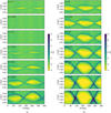 |
Fig. 1 Series of M–a FLI maps of the 5:2 MMR with Jupiter for (a) (i, ω, Ω) = (0°, 0°, 0°) and (b) (i, ω, Ω) = (30°, 180°, 60°). The eccentricity is specified in the top left corner of each map. The maps were computed for 4 kyr on a grid of 180 × 100 initial conditions, with a semi-major axis, a ∈ 〈2.805, 2.85〉 au, and mean anomaly, M ∈ 〈0°, 360°〉. The colour scale represents FLI values determined as a maximum from values obtained for six different initial deviation vectors. Stable particles are yellow, while the most chaotic ones are dark blue. |
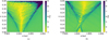 |
Fig. 2 Examples of a–e FLI maps. Panel a: ‘V-shaped’ map for (i, ω, Ω, M) = (0°, 300°, 240°, 270°). Panel b: ‘X-shaped’ map for (i, ω, Ω, M) = (20°, 36°, 240°, 30°). |
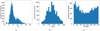 |
Fig. 3 Panel a: distribution of FLI of selected particles. Panel b: initial distribution of semi-major axis, a, of selected particles. Panel c: initial distribution of mean anomaly, M, of selected particles. |
Fraction of particles reaching a < 2 au, a < 1 au, and q < 0.005 au registered in Gladman et al. (1997); Bottke et al. (2002a); Todorović (2017) and this work.
4 Results and discussion
As was mentioned in Sect. 1, the 5:2 MMR with Jupiter has already been studied from several points of view. In this work we want to repeat to a great extent the results of Todorović (2017), while considering a greater portion of the resonance. We would like to check if it is a general characteristic of the 5:2 MMR to eject particles out from an unknown direction defined by q ≃ 0.26 au. In addition, we also want to confront our simulations with discovered PHAs and L chondrite pedigree meteorites.
This study is based on numerical simulations, and therefore it is inevitable that various simplifications and assumptions had to be made. We used a simplified model of the Solar System consisting of the Sun and all major planets. None of the large asteroids in the main asteroid belt were taken into account. These bodies were treated as active (massive) particles and initial conditions for them were set according to JPL’s Horizons System. It is important to note that non-gravitational effects were not included in our integrations, even though it is also true that we intentionally focused on gravitational interactions because we assumed that unstable particles that will interact with the resonance almost immediately are affected mainly by gravitational perturbations. Basically, we were not interested in a long-term evolution of any particle near the 5:2 MMR; we wanted to reveal the abilities of this resonance if its strong action region was encountered. We also assumed that initial conditions that lead to high FLI values during the short-term mapping of the resonance will interact with the resonance quickly. All of these simplifications and assumptions may have influenced the results of the study.
During processing of the data from our simulations, we found out that some results are similar to the results of Todorović (2017); however, we also found a lot of differences. We do not know what is the cause of these differences, but several possible reasons come to mind. The obvious one is that we tried to map a greater portion of the resonance; however, there are also other options such as the choice of simulation parameters or the way of choosing initial conditions for the simulations. Specific similarities and differences are introduced in the following four subsections.
4.1 Transportation to the NEO region
The limit for reaching the NEO region – that is, the perihelion distance, q < 1.3 au – was fulfilled by 99.45% of the test particles in our simulation. Specifically, 10 025 out of 10 080 test particles became NEOs at some point during the integration. A practically identical percentage of test particles also became NEOs in the work of Todorović (2017). Such a large amount was not observed in earlier studies (e.g. Gladman et al. 1997; Bottke et al. 2002a). As Todorović (2017) stated, such a disagreement can be primarily attributed to the way the initial conditions were chosen (only unstable particles were selected).
According to JPL’s Center for Near-Earth Object Studies (CNEOS)1, near-Earth asteroids (NEAs) can be divided into four main groups:
Amors (a > 1.0 au, 1.017 < q < 1.3 au),
Apollos (a > 1.0 au, q < 1.017 au),
Atens (a < 1.0 au, Q > 0.983 au), and
Atiras (a < 1.0 au, Q < 0.983 au),
where Q represents the aphelion distance. Cumulative numbers of particles reaching individual groups of NEAs in our simulation are given in Fig. 4. Total numbers of particles reaching these four groups are 10 025 (99.45%), 9 957 (98.78%), 875 (8.68%), and 474 (4.70%), respectively. However, most of test particles that reached Aten or Atira region (for the first time) had an eccentricity of e > 0.96; that is, these particles were almost hyperbolic. Some of these particles reached these types of orbit in the final stages of their evolution – only a few hundred years before they were ejected to hyperbolic orbit or to an orbit with a > 100 au. Many of them evolved further for a longer period of time after reaching an Aten- or Atira-type of orbit, but only several of them survived a whole integration for 10 Myr. If we omitted particles with e > 0.96, we would obtain only 12 particles that reached the Aten region and 12 particles that reached the Atira region. The first entries into these NEA groups are recorded at 2500, 14 500, 166 100, and 236700 yr, respectively, and the median times of first entries are 0.31, 0.49, 2.1, and 2.1 Myr, respectively. In comparison to Todorović (2017), we registered a significantly smaller number of Aten-group objects (in Todorović 2017 it was 22.5% of test particles). Time values corresponding to various NEA groups are considerably different from values obtained by Todorović (2017).
According to our simulation, the time at which 50% of test particles became NEOs - that is, the median time – is ~0.31 Myr. The average time of the first entry into the NEO region is ~0.62 Myr. These values are slightly higher than in Todorović (2017). As Todorović (2017) illustrates, estimating the mean lifetime that an object spends in the NEO region is tricky because the majority of test particles undergo multiple entries into the NEO region. Based on our simulation, the mean value of the first stay of a particle in the NEO region is very short, only ~430 yr; on the other hand, the mean value of the longest stay is ~0.27 Myr. The value corresponding to the longest stay is similar to the results from Todorović (2017) and Bottke et al. (2002a), where the authors estimated times of 0.2 and 0.19 Myr, respectively. The average time that a particle (which managed to become an NEO) spends in the NEO region was estimated to be ~0.69 Myr.
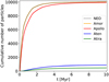 |
Fig. 4 Cumulative numbers of particles that reached q < 1.3 au, divided into four main groups: Amors, Apollos, Atens, and Atiras. A single particle could enter several NEA groups. First entries into these groups are registered at 2 500, 14 500, 166 100, and 236 700 yr, the median times of those entries are approximately 0.31, 0.49, 2.1, and 2.1 Myr, and the total numbers of bodies reaching these groups are 10 025, 9 957, 875, and 474, respectively. |
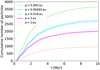 |
Fig. 5 Cumulative numbers of particles with a reduced semi-major axis or migrating closer to the Sun, i.e. particles reaching a < 2 au, a < 1 au, q < 0.005 au, q < 0.00465 au, and q < 0.016 au. First entries into these zones are registered at 129 200, 166 100, 130 100, 130 100, and 119 600 yr, the median times of the first entries are 1.9, 2.1, 2.0, 2.0, and 1.8 Myr, and the total number of particles reaching these regions are 2002, 951 , 2762, 2678, and 3648. |
4.2 Migration to the Sun
A relatively large number of test particles in our simulation also migrated closer to the Sun. Table 2 in the paper by Todorović (2017) can be expanded by adding our results – see Table 1. According to older studies, the 5:2 MMR was not capable of driving bodies to orbits with semi-major axis a < 1 au. Our study and the study of Todorović (2017) report a different result. During our simulation, 9.43% of test particles reached the a < 1 au region. In the case of reaching a < 2 au, we registered 19.86%. However, the percentage of particles that reached those regions in our simulation is lower than in Todorović (2017), especially in the case of a < 1 au.
Todorović (2017) defined the Sun-grazing bodies as bodies that have perihelion distances smaller than 0.005 au. During our simulation, 2762 test particles (27.4%) entered the region q < 0.005 au, which is much more than in previous studies. In Fig. 5, this result is demonstrated. Unlike in Todorović (2017), in Fig. 5 we can see that the curve for q < 0.005 au is above the curves for a < 2 au and a < 1 au. The vast majority of these particles reached this type of orbit by increasing in eccentricity close to the value of 1, only several of them also experienced a dramatic decrease in the semi-major axis. Only eight particles that reached this region had a < aMercury ≈0.3871 au2 and none of them had a < 0.1 au. Moreover, the majority of Sun-grazing particles (according to the definition mentioned in Todorović 2017) reached this kind of orbit for the first time at the final stage of their evolution. 2235 out of 2762 particles remained in the simulation for less than 1000 yr, before they were ejected to hyperbolic orbit or to an orbit with a semi-major axis larger than 100 au. However, 15 of these 2762 particles finished the whole 10 Myr simulation and ended on an orbit with 0 < a < 100 au (i.e. they were not ejected).
One can find different definitions of Sun-grazing objects, though. For example, Jones et al. (2018) defined a Sun-grazing object in the case of q < 3.45 R⊙ ≈ 0.016 au and a so-called Sun-diving object (or Sun impactor) when q < R⊙ ≈ 0.00465 au (where R⊙ represents the radius of the Sun). If we use this definition, we will get 3 648 (36.19%) Sun-grazing particles in our simulation. For more details on the timing of the first entries into a < 2 au, a < 1 au, q < 0.005 au, q < 0.00465 au, and q < 0.016 au regions and the total number of particles reaching these criteria, see the caption of Fig. 5.
Radii of Hill spheres (rHill) and corresponding percentage of test particles entering the Hill sphere in both work of Todorović (2017) and this work.
4.3 Close encounters with the planets
As was mentioned before, during the integration we also tracked close encounters of test particles with the planets. This time, we took a slightly different approach than Todorović (2017) to obtain the same kind of information. Our software does register collisions, so we decided to use this fact to count close approaches to the planets. The Hill sphere is a region around a planetary body where its own gravity plays a dominant role compared to other nearby bodies, including the Sun. While Todorović (2017) decided to use one value of the Hill sphere radius for all terrestrial planets and another for all Jovian planets, we wanted to use more realistic values of the Hill sphere radius. In our case, each of the planets was assigned a radius equal to its Hill sphere, which was estimated using the well-known formula
 (4)
(4)
where m⊙ is the mass of the Sun, mpl the mass of the planet, and apl the semi-major axis of the planet. Under such conditions, we registered direct collisions of test particles with the planets. However, these collisions were resolved only by saving the information about which objects collided; these collisions had no effect on the orbital evolution of the planets or test particles. Corresponding radii of Hill spheres and the percentage of particles entering the Hill sphere of each planet are given in Table 2. The table also contains results and radii of Hill spheres considered in Todorović (2017). The last column of Table 2 also contains percentages of test particles that encountered with a given planet as a first planet in the simulation. We can see that the first encounters of test particles with a planet usually involved a terrestrial planet.
We expected to obtain similar results to Todorović (2017), where Jupiter dominated, with 98.5% of particles entering its Hill sphere and the number of bodies approaching other planets decreasing gradually as we move away from Jupiter, both inwards and outwards. Surprisingly, our result was anomalous. According to our simulation, Earth dominates. The amount of test particles entering the Hill sphere of the Earth is 92.8%. Then Jupiter follows, with 89.5% of particles approaching it. This discrepancy may be caused by considering different Hill spheres, slightly larger for the Earth and approximately twice as small for Jupiter, compared to Todorović (2017) (see Table 2). Based on our simulation, 69 test particles (0.7%) underwent no close encounter with a planet, which is roughly the same amount as in Todorović (2017). In general, these results, whether ours or Todorović’s, show that a test particle usually encountered several planets before its final state. Various gravitational interactions can lead to various evolutions. However, a possible outcome of a very close encounter with a planet (or the Sun) is an inscrutable evolution. Therefore, the overall dynamical behaviour of such particles can be described as traveling through the interplanetary space governed by subsequent close encounters (or perhaps captures into other resonances) until the collision with a planet or the Sun occurs, or alternatively until the ejection from the Solar System. We could probably say that overall evolution of these particles is practically chaotic. We remark that real collisions were not registered during our simulations.
4.4 Final destinations of test particles
The orbital evolution of test particles in our simulation was diverse. Even though we selected only the most unstable particles (with the highest FLI values according to our maps), a few of them had a completely stable evolution. Simulations for only 436 particles (4.33%) were not stopped before finishing 10 Myr. In 3602 cases (35.73%) the simulation was stopped because the particle reached hyperbolic orbit; that is, e > 1. The remaining 6042 particles (59.94%) managed to reach an orbit with a > 100 au. Todorović (2017) registered approximately the same percentages, while integrating only up to 5 Myr. Initial and final distributions of test particles in our simulation are given in Fig. 6. The red and green dots in the figure represent the positions from which the particles were ejected to hyperbolic orbit or to an orbit with a > 100 au. As we can see, red and green dots are mostly located along (or in between) the lines representing (a, e) locations with a perihelion (or aphelion) distance equal to the perihelion (or aphelion) distance of Jupiter. So, we can assume (like Todorović 2017) that Jupiter caused the majority of those ejections. However, the effect of other planets cannot be ruled out completely either.
In comparison to Fig. 6 from Todorović (2017), in the bottom panel of our Fig. 6 we can see that a lot of red, and also some of the green, dots lie along e ≈ 1, near the hyperbolic limit. We register 2 839 test particles as having e > 0.98 before the ejection. We also find that particles that got close to the Sun reached their orbit by increasing the eccentricity close to 1 (see Sect. 4.2). So, we assume that the majority of particles placed along e ≈ 1 are particles that reached very small perihelion distances. This fact was also confirmed when we plotted the final state distribution of particles that were able to reach q < 0.005 au and that were unable to reach such a perihelion distance, separately. It should be noted that the evolution of a particle after a close approach to the Sun is at least uncertain. Since our integrations were not detecting real collisions, we can only suppose that at least several of these particles reaching close to the Sun would finish their evolution by impacting the Sun.
However, what is more interesting for us, in Fig. 6, is that we do not see eliminations along the line q = 0.26 au (orange line), as were found in Todorović (2017). More precisely, there are several particles ejected from the positions close to the line representing q = 0.26 au; however, when we take a closer look at evolution of our test particles, we find out that none of them is evolving along q ≃ 0.26 au (as can be seen in Fig. 7 in Todorović 2017). Several particles are seemingly evolving along a line that could be defined by some value of perihelion distance, but not q ≃ 0.26 au (see for example Fig. 8a).
Examples of the evolution of five test particles are given in Figs. 7 and 8. All of these particles started their evolution with an increasing eccentricity and a semi-major axis that remained constant. The first particle (Fig. 7a) survived a whole simulation for 10 Myr and stayed in the NEO region for most of its lifetime. The particle in Fig. 7b experienced a rapid evolution along the line representing the perihelion distance of Jupiter and was ejected to an orbit with a > 100 au. The third particle (Fig. 7c) reached a low perihelion distance and stayed in the simulation for almost 4 Myr before it was ejected to a hyperbolic orbit from the position with e ≈ 1. As we mentioned in the previous paragraph, the particle in Fig. 8a was seemingly evolving along the line that could represent some fixed perihelion distance; however, this line is located far from q ≃ 0.26 au. At the end of the simulation this particle got to an orbit with a > 100 au. Last particle (Fig. 8b) also survived whole simulation, however this particle ended up in the region typical for centaurs. Test particles with these types of evolution are found multiple times in our simulation.
Figure 9 gives the end-state distribution of all test particles again, but this time the colour represents the lifetime of the test particles. We can see that particles that stayed in the simulation for the whole 10 Myr (dark blue triangles) are mostly placed in two regions, in front of and then behind the region delimited by the perihelion distance of Saturn, qS at, and the aphelion distance of Jupiter, QJup. On the other hand, most particles ejected to a hyperbolic orbit or to an orbit with a > 100 au terminated their evolution relatively early (predominantly yellowish and greenish colours) compared to the complete 10 Myr. The median lifetime of a particle that reached e > 1 or a > 100 au is ~1.4 Myr according to our simulation. The mean lifetime of such a particle is ~2 Myr. These relatively short mean and median lifetimes in conjunction with the timings of the first entries into different NEA regions or the near-Sun space (see the first two subsections of Sect. 4) tell us that a particle that encountered a strong action region of the 5:2 MMR can evolve rapidly and its orbit can change significantly within a relatively short period of time. This is another indication that these particles evolve in an unstable manner in general.
We also wanted to know if there are any similarities in orbital evolution or final state of particles with similar FLI values or with the same initial eccentricity, inclination, argument of perihelion, or longitude of ascending node. The only thing that immediately emerged is that simulations of particles with the initial inclination i = 30° took longer and a larger number of these particles also survived the whole integration for 10 Myr. In comparison to other values of initial inclination, there were 68, 58, 85, and 225 survivors in the case of i = 0°, i = 10°, i = 20°, and i = 30°, respectively. Our results also show that being ejected to hyperbolic orbit is more probable for particles with higher initial inclinations, whereas reaching an orbit with a > 100 au is more probable for particles with lower initial inclinations. In our simulation 1979, 1827, 1342, and 894 test particles were driven to a > 100 au, while 473, 635, 1093, and 1401 particles were ejected to hyperbolic orbit for the initial inclinations 0°, 10°, 20°, and 30°, respectively.
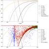 |
Fig. 6 Initial (top) and final (bottom) distribution of test particles in our simulation. Green and red dots in the final distribution represent the positions from which the particles were ejected to hyperbolic orbits (red dots) and orbits with a > 100 au (green dots), whereas particles that survive whole simulation for 10 Myr are blue. Black lines represent the sets of (a, e) where a particle can be to have a perihelion (or aphelion) distance equal to the perihelion (or aphelion) distance of one of the planets. Planets are specified in the legend. For example, qJup represents the perihelion distance of Jupiter, QJup the aphelion distance of Jupiter, etc. The orange line represents the perihelion distance of q = 0.26 au. |
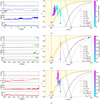 |
Fig. 7 Orbital evolution of three test particles. The left panels represent the evolution of the semi-major axis, a, eccentricity, e, inclination, i, and perihelion distance, q, with time. The colours of the lines represent the final state of the particle, as in Fig. 6, i.e. red = a hyperbolic orbit, green = an orbit with a > 100 au, and blue = a survivor for 10 Myr. The dashed black line inside the graph for q represents q = 1.3 au. The right panels represent the evolution of the particle from the left panel in the (a, e) plane. The initial state is represented by a cyan star and the final position by a magenta cross. The yellow area delimits the NEO region with q < 1.3 au. Pink, magenta, and brown lines divide the NEO region into four main groups: R = amoRs, O = apollOs, N = ateNs, and A = atirAs. The colour bar represents the lifetime of the particle, i.e. a different time interval for each particle. Panel a: particle with initial values (a, e, i, ω, Ω, M, FLI) = (2.8250 au, 0.15, 0°, 0°, 0°, 162.9050°, 6.2225). Panel b: (a, e, i, ω, Ω, M, FLI) = (2.8241 au, 0.1, 10°, 120°, 180°, 18.1006°, 7.0004). Panel c: (a, e, i, ω, Ω, M, FLI) = (2.8359 au, 0.2, 0°, 0°, 300°, 225.2514°, 7.9464). |
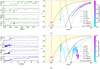 |
Fig. 8 Orbital evolution of another two test particles (as in Fig. 7). Panel a: particle with initial values (a, e, i, ω, Ω, M, FLI) = (2.8355 au, 0.3, 0°, 120°, 240°, 305.6983°, 10.7727). Panel b: (a, e, i, ω, Ω, M, FLI) = (2.8273 au, 0, 10°, 0°, 60°, 60.3352°, 6.6942). |
4.5 Potentially hazardous objects
As we mentioned in Sect. 4.3, a large number of test particles in our simulation entered the Hill sphere of the Earth; that is, got to the Earth itself closer than ~0.01 au (see Table 2). This fact guided us to search for PHA-like orbits in our simulation.
Potentially hazardous asteroids are currently defined3 based on parameters that evaluate the potential of the object to make a threatening close approach to the Earth. Specifically, all asteroids with a minimum orbit intersection distance (MOID) with respect to the Earth of 0.05 au or less and an absolute magnitude of H ≤ 22.0 are considered PHAs. In other words, asteroids that cannot get any closer to the Earth than 0.05 au or that are smaller than ~140 m in diameter (an albedo of 14% is assumed) are not considered PHAs.
In our simulation we registered at least 9823 test particles (97.45%) on a PHA-like orbit with MOID ≤ 0.05 au. This is only the minimal total number, because the calculation of MOID for every particle every 100 yr was very time-consuming, so we decided to calculate MOID only every 2 500 yr. The calculation of MOID every 100 yr was made only for 70 particles selected from seven FLI maps given in Fig. 1a, to check if we were not missing too many test particles with MOID ≤ 0.05 au. This calculation showed that from these 70 particles we missed only one particle with MOID ≤ 0.05 au. A particle satisfying this criterion of PHAs was for the first time registered at 32 500 yr. In Fig. 10, we can see the cumulative number of particles reaching MOID ≤ 0.05 au. For comparison, in the figure there are also curves for cumulative numbers of NEOs, particles ending on an orbit with a > 100 au and particles reaching hyperbolic orbit. Other details about timing can be found in the caption of Fig. 10.
Previous studies mainly investigated the connection of the 5:2 MMR with asteroid 3200 Phaethon (1983 TB). However, our results show that it is relatively easy for a particle from the 5:2 MMR to reach a PHA-like orbit. We decided to count test particles recovering the orbit of any of the currently known PHAs. We considered a list of 2374 PHAs, which we obtained from JPL’s Small-Body Database4. We searched for test particles in our simulation that at some moment of the integration satisfy analogous criteria as in Todorović (2017) or Todorović (2018); that is, |a - − aPHA| < 0.1 au, |e − ePHA| < 0.1, and |i − iPHA| < 3°, where (aPHA, ePHA, iPHA) represent orbital elements corresponding to any of the PHAs.
The most frequently found PHAs are listed in Table 3. For the complete table, containing all considered PHAs, see supplementary material available online at the CDS. As can be seen, at least 7605 (75.45%) test particles recovered the orbit of asteroid 442037 (2010 PR66) at some moment of the integration. On the other hand, in the case of 153 PHAs (6.44% of considered PHAs), none of the test particles recovered their orbit. We were also interested in PHAs mentioned in Sect. 1. According to our simulation, 4180 (41.47%) particles reached the orbit of asteroid 214869 (2007 PA8) at some point during the simulation. However, only 172 (1.71%) test particles recovered the orbit of 3200 Phaethon (1983 TB). Of course, Table 3 is not direct proof that the PHAs listed in the table came to the Earth via the 5:2 MMR with Jupiter. It tells us that if a particle encounters the unstable region of 5:2 MMR, it is relatively easy to reach such an orbit.
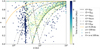 |
Fig. 9 Final distribution of test particles. The colour of marker corresponds to the time that particles spend in the simulation, i.e. their lifetime. Dots represent particles that reached an orbit with a > 100 au, crosses represent hyperbolic orbits, and triangles represent survivors. |
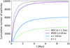 |
Fig. 10 Cumulative numbers of test particles reaching q < 1.3 au, MOID ≤ 0.05 au, a > 100 au, and e > 1 (alternatively a < 0 au). First entries into these zones are registered at 2 500, 32 500, 63 600, and 67 900 yr, the median times of those first entries are approximately 0.31, 0.50, 1.2, and 1.6 Myr, and the total numbers of bodies reaching these zones are 10 025, 9823, 6042, and 3602, respectively. |
PHAs whose orbits are most frequently found among the test particles in our simulation.
4.6 L chondrite meteorites with pedigree
As was mentioned in Sect. 1, there is a hypothesis that fossil L chondrite meteorites could have been delivered to the Earth via the 5:2 MMR with Jupiter. So, we decided to also search for orbits associated with recent L chondrite meteorites in our simulation. The procedure was the same as in the case of PHA-like orbits. In total, we considered 20 pedigree meteorites5 that were identified as L or L/LL5 type. We searched for test particles in our simulation that satisfy the same criteria as in the previous section; that is, |a − amet| < 0.1 au, |e − emet| < 0.1, and |i − imet| < 3°, where (amet, emet, imet) represent orbital elements of heliocentric orbit of any of the considered meteorites.
The results are listed in Table 4. The numbers are not as high as in the case of PHAs. We can see that 1087 test particles (10.78%) recovered the orbit of the Porangaba meteorite that fell in 2015 in Brazil. At the opposite end of the list is the Madura Cave meteorite, whose fall was registered in Australia in 2020. The heliocentric orbit of this meteorite was recovered only by two test particles in our simulation.
5 Possible sink at q ≃ 0.26 au
An unexpected result of Todorović (2017) was that, in addition to the main removal course of 5:2 MMR caused by Jupiter, most test particles were ejected out from an unknown direction along the orbits with q ≃ 0.26 au. However, dynamical origin of this elimination was also unknown. The same result (elimination course along q ≃ 0.26 au) was also observed for other two sets of (i, ω, Ω, M). Todorović (2017) suggested that the line at q ≃ 0.26 au might be a natural inner stability border of the NEO region. This line was identified as so-called sink of the 5:2 MMR with Jupiter; in other words, a dynamical route along which most particles escape from the Solar System or fall into the Sun.
As we mentioned in Sect. 4.4, we did not manage to obtain the same result in our simulation. So, we started to search for possible reasons. The first obvious difference between our simulation and the simulation of Todorović (2017) is the software we used to perform integrations. We used WHFast and MERCURIUS integrators (REBOUND package), while Todorović (2017) used ORBIT9 integrator (OrbFit package). Another evident difference is the epoch for which the integrations were performed. In our simulation, we set the initial distribution of perturbing bodies to the date June 1 2023 at 00:00. The epoch in the work of Todorović (2017) was JD 245 6200 (September 29 2012 at 12:00). In our case, the FLI maps were computed for 4 kyr, while the FLI maps in Todorović (2017) were computed for 10 kyr, suggesting that Todorović (2017) might have also detected different particles that became unstable later -after 4 kyr, but before 10 kyr. In both cases, all the planets in the Solar System were taken into account; however, in Todorović (2017) the mass of Mercury was added to the mass of the Sun and the corresponding barycentric correction was applied to the initial conditions. Moreover, we selected only the ten most unstable particles from each of the FLI maps, whereas Todorović (2017) selected 1000 test particles based on a single FLI map, so their integrations also contained some slightly more stable particles.
We verified whether we were able to obtain the same results as Todorović (2017). Other simulations were arranged and this time we used the same epoch as Todorović (2017): JD 245 6200. One of the simulations was integrated for 4 kyr and the other for 10 kyr by the WHFast integrator. Integrations were focused only on the part of the 5:2 MMR from which Todorović (2017) selected test particles; that is, a ∈ 〈2.82, 2.834〉 au and e ∈ 〈0, 0.22〉. In both cases, the a-e FLI map was computed (on a grid of 200 × 250 test particles) and the remaining orbital elements were fixed to values according to Todorović (2017); that is, (i,ω, Ω, M) = (10°, 70°, 260°, 99°). The resulting FLI maps are given in Fig. 11. Both of the FLI maps have the same general structure; however, in the case of the map computed for 10 kyr (Fig. 11b) we can also see a lot of peculiar structures inside the resonance. In general, the map in Fig. 11b is very similar to the map from Todorović (2017); however, one obvious difference can be spotted - the range of obtained FLI values.
Different FLI values suggest that there is some difference in calculating FLI. It is a bit questionable which logarithm should be used to calculate FLI – natural or decadic – however, in our opinion this should not play an important role in comparing particles within the same FLI map. Of course, the values in the case of a natural logarithm would be different than in the case of a decadic logarithm; however, when we look at the definition of FLI (Eq. (3)), it looks like the logarithm is used only to make extremely large numbers smaller and more comparable. Another question is which initial deviation vector(s) was (were) used by Todorović (2017), and how the variational equations are treated within the OrbFit package. Although there is a difference in the ranges of FLI values, we believe that our FLI map in Fig. 11b and the map from Todorović (2017) are equivalent when they are used to compare the instability of particles within the map (the structures in our map are generally the same as in the map of Todorović 2017).
The verification continued with the selection of the 500 most unstable test particles from both maps in Fig. 11. These particles were integrated by the MERCURIUS integrator for 5 Myr (as in Todorović 2017). This time, we were not interested in any specific statistical details; we only wanted to see the final distribution of test particles. The final distribution of test particles in both cases is displayed in Fig. 12. Surprisingly, none of the panels in Fig. 12 contains an elimination course along q ≃ 0.26 au; however, elimination along e = 1 is present in both cases (unlike in Todorović 2017).
Although the first attempt to reproduce the results of Todorović (2017) was not successful, we made another one. Todorović (2017) listed (in supplementary materials) all 1000 test particles that she selected from the FLI map. We integrated these particles using the MERCURIUS integrator for 5 Myr and for the epoch JD 245 6200. The resulting final distribution of test particles is given in Fig. 13. However, massive ejection along q ≃ 0.26 au is not present in this case either. We can see that only two of the ejected particles lie on the orange line representing q = 0.26 au. However, we do not know if they were also evolving along the orange line before the ejection. Anyway, only two particles is too few; it could still be a coincidence. We also tried to plot the ‘final’ distribution, for example 5 kyr or 10 kyr before our final states, to check if the reason could be as simple as that; however, still no elimination along q ≃ 0.26 au was present. We also repeated the simulation of those 1000 particles, while omitting Mercury from the simulation completely. In this case, only one test particle was ejected from the position close to the line representing q = 0.26 au.
Unfortunately, we were not able to reproduce the results of Todorović (2017) and confirm eliminations along q ≃ 0.26 au. The only differences (from the differences mentioned above) that are left are different software used for the integrations and the way that the planet Mercury was treated in simulations.
Meteorites whose heliocentric orbit was searched for among the test particles in our simulation.
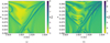 |
Fig. 11 a–e FLI maps of the part of the 5:2 MMR with Jupiter, a ∈ 〈2.82, 2.834〉 au and e ∈ 〈0, 0.22〉. The maps were computed on a grid of 200 × 250 initial conditions and the remaining orbital elements were fixed to (i, ω, Ω, M) = (10°, 70°, 260°, 99°). The colour scale represents FLI values determined as a maximum from values obtained for six different initial deviation vectors. Stable particles are yellow, while most chaotic ones are dark blue. The maps were computed for (a) 4 kyr and (b) 10 kyr. |
6 Conclusion
In this work we dealt with the transportation abilities of the 5:2 MMR with Jupiter. We compared our results with previous studies, especially the study of Todorović (2017) that used a very similar method. In this paper, the FLI map method was applied to the region of the 5:2 MMR. In total, we used 1008 M–a FLI maps for various initial sets of (e, i, ω, Ω), to examine a greater portion of the resonance than Todorović (2017). These FLI maps enabled us to differentiate between stable and unstable initial conditions. Based on our FLI maps, we selected 10 080 unstable test particles and integrated them up to 10 Myr.
Our results in some aspects correspond to the results of Todorović (2017). For example, according to our simulation, 99.45% of test particles became NEOs at some point during the integration, which is much more than what was found in the older studies. However, this can be attributed to the method that was used in Todorović (2017) and this work. Nevertheless, there are also many different results. We obtain considerably smaller amount of particles reaching a < 1 au, although this amount is still considerably greater than in older studies. In addition, we register that 27.4% of particles reached an orbit with q < 0.005 au, which is again much more than in any of the previous studies. In our simulation, the vast majority of test particles entered the Hill sphere of the Earth (92.8%). The amount of particles that got as close to the orbit of Earth as PHAs was, of course, even larger (97.45%). This large amount, in conjunction with the result of Granvik et al. (2018) that the 5:2 MMR contributes to the NEO population primarily at larger sizes, led us to search for orbits corresponding to the known PHAs. According to our simulation, the orbits of 17 known PHAs were recovered by at least 70% of the test particles at some point. We also searched for heliocentric orbits of recent L chondrite meteorites among test particles in our simulation. Only in the case of the Porangaba and Park Forest meteorites did more than 10% of test particles recover their orbit at some point during the integration.
The final distribution of test particles in our simulation reveals that ejections to hyperbolic orbits or to orbits with a > 100 au were predominantly caused by Jupiter, as was expected. However, we also find numerous removals along the line e = 1. These are mostly cases of particles that reached low perihelion distances. Unfortunately, our simulation did not confirm the existence of a removal course along q ≃ 0.26 au. We also tried to repeat the procedures of Todorović (2017) while using different software, to see if we were able to obtain ejections along q ≃ 0.26 au. However, our attempts were not successful; there is some kind of discrepancy that is definitely worth further investigation. Checking the procedures using other integrators (e.g. from the MERCURY package) could also be beneficial.
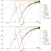 |
Fig. 12 Final distribution of 500 test particles selected based on the FLI map computed for 4 kyr (top) and for 10 kyr (bottom). Green and red dots represent the positions from which the particles were ejected to hyperbolic orbits (red dots) and orbits with a > 100 au (green dots), whereas particles that survive the whole simulation for 5 Myr are blue. Black lines represent the perihelion and aphelion distances of selected planets. The orange line represents the perihelion distance, q = 0.26 au. |
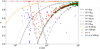 |
Fig. 13 Final distribution of 1000 test particles that were selected by Todorović (2017) and integrated by MERCURIUS integrator for 5 Myr. Green and red dots represent the positions from which the particles were ejected to hyperbolic orbits (red dots) and orbits with a > 100 au (green dots), whereas particles that survive the whole simulation for 5 Myr are blue. Black lines represent the perihelion and aphelion distances of selected planets. The orange line represents the perihelion distance, q = 0.26 au. |
Acknowledgements
The author would like to express her gratitude to Dr. Leonard Kornoš, Dr. Luboš Neslušan and the anonymous referee for their comments and suggestions, which definitely helped to improve the paper. This work was supported by the VEGA – the Slovak Grant Agency for Science, grant No. 2/0009/22.
References
- Andrade, M., Docobo, J. A., García-Guinea, J., et al. 2022, MNRAS, 518, 3850 [CrossRef] [Google Scholar]
- Bottke, W. F., Morbidelli, A., Jedicke, R., et al. 2002a, Icarus, 156, 399 [NASA ADS] [CrossRef] [Google Scholar]
- Bottke, W. F., Vokrouhlický, D., Rubincam, D. P., & Broz, M. 2002b, in Asteroids III, 395 [CrossRef] [Google Scholar]
- Brown, P., Pack, D., Edwards, W. N., et al. 2004, Meteor. Planet. Sci., 39, 1781 [NASA ADS] [CrossRef] [Google Scholar]
- Brown, P. G., McCausland, P. J. A., Hildebrand, A. R., et al. 2023, Meteor. Planet. Sci., 58, 1773 [CrossRef] [Google Scholar]
- Ceplecha, Z., & Revelle, D. O. 2005, Meteor. Planet. Sci., 40, 35 [NASA ADS] [CrossRef] [Google Scholar]
- de León, J., Campins, H., Tsiganis, K., Morbidelli, A., & Licandro, J. 2010, Astron. Astrophys., 513, A26 [CrossRef] [EDP Sciences] [Google Scholar]
- Devillepoix, H. A. R., Sansom, E. K., Bland, P. A., et al. 2018, Meteor. Planet. Sci., 53, 2212 [NASA ADS] [CrossRef] [Google Scholar]
- Devillepoix, H. A. R., Sansom, E. K., Shober, P., et al. 2022, Meteor. Planet. Sci., 57, 1328 [NASA ADS] [CrossRef] [Google Scholar]
- Dvorak, R., Pilat-Lohinger, E., Funk, B., & Freistetter, F. 2003, A&A, 398, L1 [NASA ADS] [CrossRef] [EDP Sciences] [Google Scholar]
- Ferus, M., Petera, L., Koukal, J., et al. 2020, Icarus, 341, 113670 [NASA ADS] [CrossRef] [Google Scholar]
- Froeschlé, C., Lega, E., & Gonczi, R. 1997, Celest. Mech. Dyn. Astron., 67, 41 [CrossRef] [Google Scholar]
- Froeschlé, C., Guzzo, M., & Lega, E. 2000, Science, 289, 2108 [CrossRef] [Google Scholar]
- Gardiol, D., Barghini, D., Buzzoni, A., et al. 2021, MNRAS, 501, 1215 [Google Scholar]
- Gladman, B. J., Migliorini, F., Morbidelli, A., et al. 1997, Science, 277, 197 [NASA ADS] [CrossRef] [Google Scholar]
- Granvik, M., & Brown, P. 2018, Icarus, 311, 271 [Google Scholar]
- Granvik, M., Morbidelli, A., Jedicke, R., et al. 2018, Icarus, 312, 181 [CrossRef] [Google Scholar]
- Guzzo, M. 2006, Icarus, 181, 475 [NASA ADS] [CrossRef] [Google Scholar]
- Halliday, I., Blackwell, A. T., & Griffin, A. A. 1978, J. Roy. Astron. Soc. Canada, 72, 15 [Google Scholar]
- Jenniskens, P., Rubin, A. E., Yin, Q.-Z., et al. 2014, Meteor. Planet. Sci., 49, 1388 [NASA ADS] [CrossRef] [Google Scholar]
- Jenniskens, P., Utas, J., Yin, Q.-Z., et al. 2019, Meteor. Planet. Sci., 54, 699 [CrossRef] [Google Scholar]
- Jones, G. H., Knight, M. M., Battams, K., et al. 2018, Space Sci. Rev., 214, 20 [NASA ADS] [CrossRef] [Google Scholar]
- Kartashova, A., Golubaev, A., Mozgova, A., et al. 2020, Planet. Space Sci., 193, 105034 [CrossRef] [Google Scholar]
- Korochantseva, E. V., Trieloff, M., Lorenz, C. A., et al. 2007, Meteor. Planet. Sci., 42, 113 [NASA ADS] [CrossRef] [Google Scholar]
- Kővágó, G. 2021, eMeteorNews, 6, 87 [Google Scholar]
- Kováčová, M., Kornoš, L., & Matlovic, P. 2022, MNRAS, 509, 3842 [Google Scholar]
- Lega, E., Guzzo, M., & Froeschlé, C. 2016, Theory and Applications of the Fast Lyapunov Indicator (FLI) Method, eds. C. H. Skokos, G. A. Gottwald, & J. Laskar (Berlin, Heidelberg: Springer Berlin Heidelberg), 35 [Google Scholar]
- Malhotra, R. 1998, in ASP Conf. Ser., 149, Solar System Formation and Evolution, eds. D. Lazzaro, R. Vieira Martins, S. Ferraz-Mello, & J. Fernandez, 37 [NASA ADS] [Google Scholar]
- Malhotra, R. 2022, in Multi-Scale (Time and Mass) Dynamics of Space Objects, 364, eds. A. Celletti, C. Gales, C. Beaugé, & A. Lemaître, 85 [NASA ADS] [Google Scholar]
- Meier, M. M. M., Gritsevich, M., Welten, K. C., et al. 2020, in Eur. Planet. Sci. Congress, EPSC2020-730 [Google Scholar]
- Morbidelli, A., Bottke, W. F., Froeschlé, C., & Michel, P. 2002, in Asteroids III, 409 [CrossRef] [Google Scholar]
- Nedelcu, D. A., Birlan, M., Popescu, M., Badescu, O., & Pricopi, D. 2014, A&A, 567, A7 [NASA ADS] [CrossRef] [EDP Sciences] [Google Scholar]
- Nesvorný, D., Vokrouhlický, D., Morbidelli, A., & Bottke, W. F. 2009, Icarus, 200, 698 [CrossRef] [Google Scholar]
- Rein, H., & Spiegel, D. S. 2015, MNRAS, 446, 1424 [Google Scholar]
- Rein, H., & Tamayo, D. 2015, MNRAS, 452, 376 [Google Scholar]
- Rein, H., & Tamayo, D. 2016, MNRAS, 459, 2275 [Google Scholar]
- Rein, H., Hernandez, D. M., Tamayo, D., et al. 2019, MNRAS, 485, 5490 [Google Scholar]
- Rosengren, A. J., Daquin, J., Tsiganis, K., et al. 2017, MNRAS, 464, 4063 [CrossRef] [Google Scholar]
- Sanchez, J. A., Reddy, V., Dykhuis, M., Lindsay, S., & Le Corre, L. 2015, ApJ, 808, 93 [NASA ADS] [CrossRef] [Google Scholar]
- Schwarz, R., Haghighipour, N., Eggl, S., Pilat-Lohinger, E., & Funk, B. 2011, MNRAS, 414, 2763 [NASA ADS] [CrossRef] [Google Scholar]
- Shchekinova, E., Chandre, C., Lan, Y., & Uzer, T. 2004, J. Chem. Phys., 121, 3471 [NASA ADS] [CrossRef] [Google Scholar]
- Shrbený, L., Krzesinska, A. M., Borovicka, J., et al. 2022, Meteor. Planet. Sci., 57, 2108 [CrossRef] [Google Scholar]
- Simms, M. 2021, Geol. Today, 37, 225 [NASA ADS] [CrossRef] [Google Scholar]
- Spurný, P., Borovicka, J., Kac, J., et al. 2010, Meteor. Planet. Sci., 45, 1392 [CrossRef] [Google Scholar]
- Spurný, P., Borovicka, J., & Shrbený, L. 2020, Meteor. Planet. Sci., 55, 376 [CrossRef] [Google Scholar]
- Todorović, N. 2017, MNRAS, 465, 4441 [CrossRef] [Google Scholar]
- Todorović, N. 2018, MNRAS, 475, 601 [NASA ADS] [Google Scholar]
- Todorović, N., & Novakovic, B. 2015, MNRAS, 451, 1637 [CrossRef] [Google Scholar]
- Trigo-Rodríguez, J. M., Borovicka, J., Spurný, P., et al. 2006, Meteor. Planet. Sci., 41, 505 [CrossRef] [Google Scholar]
- Vida, D., Šegon, D., Šegon, M., et al. 2021, in Eur. Planet. Sci. Congress, EPSC2021-139 [Google Scholar]
- Villac, B. F. 2008, Celest. Mech. Dyn. Astron., 102, 29 [NASA ADS] [CrossRef] [Google Scholar]
- Vokrouhlický, D., & Farinella, P. 2000, Nature, 407, 606 [CrossRef] [Google Scholar]
- Wetherill, G. W. 1976, Geochim. Cosmochim. Acta, 40, 1297 [CrossRef] [Google Scholar]
- Wisdom, J. 1982, AJ, 87, 577 [NASA ADS] [CrossRef] [Google Scholar]
- Wisdom, J. 1983, Icarus, 56, 51 [NASA ADS] [CrossRef] [Google Scholar]
- Zuluaga, J. I., Cuartas-Restrepo, P. A., Ospina, J., & Sucerquia, M. 2019, MNRAS, 486, L69 [CrossRef] [Google Scholar]
The value of semi-major axis of Mercury was retrieved from JPL Horizons System.
The definition of PHAs was adopted from JPL CNEOS: https://cneos.jpl.nasa.gov/about/neo_groups.html
The list of PHAs (with their orbital elements) was downloaded on October 12, 2023 using JPL Small-Body Database Query: https://ssd.jpl.nasa.gov/tools/sbdb_query.html
The list of meteorites was adopted on November 2, 2023 from: https://www.meteoriteorbits.info/
All Tables
Fraction of particles reaching a < 2 au, a < 1 au, and q < 0.005 au registered in Gladman et al. (1997); Bottke et al. (2002a); Todorović (2017) and this work.
Radii of Hill spheres (rHill) and corresponding percentage of test particles entering the Hill sphere in both work of Todorović (2017) and this work.
PHAs whose orbits are most frequently found among the test particles in our simulation.
Meteorites whose heliocentric orbit was searched for among the test particles in our simulation.
All Figures
|
Fig. 1 Series of M–a FLI maps of the 5:2 MMR with Jupiter for (a) (i, ω, Ω) = (0°, 0°, 0°) and (b) (i, ω, Ω) = (30°, 180°, 60°). The eccentricity is specified in the top left corner of each map. The maps were computed for 4 kyr on a grid of 180 × 100 initial conditions, with a semi-major axis, a ∈ 〈2.805, 2.85〉 au, and mean anomaly, M ∈ 〈0°, 360°〉. The colour scale represents FLI values determined as a maximum from values obtained for six different initial deviation vectors. Stable particles are yellow, while the most chaotic ones are dark blue. |
| In the text | |
|
Fig. 2 Examples of a–e FLI maps. Panel a: ‘V-shaped’ map for (i, ω, Ω, M) = (0°, 300°, 240°, 270°). Panel b: ‘X-shaped’ map for (i, ω, Ω, M) = (20°, 36°, 240°, 30°). |
| In the text | |
|
Fig. 3 Panel a: distribution of FLI of selected particles. Panel b: initial distribution of semi-major axis, a, of selected particles. Panel c: initial distribution of mean anomaly, M, of selected particles. |
| In the text | |
|
Fig. 4 Cumulative numbers of particles that reached q < 1.3 au, divided into four main groups: Amors, Apollos, Atens, and Atiras. A single particle could enter several NEA groups. First entries into these groups are registered at 2 500, 14 500, 166 100, and 236 700 yr, the median times of those entries are approximately 0.31, 0.49, 2.1, and 2.1 Myr, and the total numbers of bodies reaching these groups are 10 025, 9 957, 875, and 474, respectively. |
| In the text | |
|
Fig. 5 Cumulative numbers of particles with a reduced semi-major axis or migrating closer to the Sun, i.e. particles reaching a < 2 au, a < 1 au, q < 0.005 au, q < 0.00465 au, and q < 0.016 au. First entries into these zones are registered at 129 200, 166 100, 130 100, 130 100, and 119 600 yr, the median times of the first entries are 1.9, 2.1, 2.0, 2.0, and 1.8 Myr, and the total number of particles reaching these regions are 2002, 951 , 2762, 2678, and 3648. |
| In the text | |
|
Fig. 6 Initial (top) and final (bottom) distribution of test particles in our simulation. Green and red dots in the final distribution represent the positions from which the particles were ejected to hyperbolic orbits (red dots) and orbits with a > 100 au (green dots), whereas particles that survive whole simulation for 10 Myr are blue. Black lines represent the sets of (a, e) where a particle can be to have a perihelion (or aphelion) distance equal to the perihelion (or aphelion) distance of one of the planets. Planets are specified in the legend. For example, qJup represents the perihelion distance of Jupiter, QJup the aphelion distance of Jupiter, etc. The orange line represents the perihelion distance of q = 0.26 au. |
| In the text | |
|
Fig. 7 Orbital evolution of three test particles. The left panels represent the evolution of the semi-major axis, a, eccentricity, e, inclination, i, and perihelion distance, q, with time. The colours of the lines represent the final state of the particle, as in Fig. 6, i.e. red = a hyperbolic orbit, green = an orbit with a > 100 au, and blue = a survivor for 10 Myr. The dashed black line inside the graph for q represents q = 1.3 au. The right panels represent the evolution of the particle from the left panel in the (a, e) plane. The initial state is represented by a cyan star and the final position by a magenta cross. The yellow area delimits the NEO region with q < 1.3 au. Pink, magenta, and brown lines divide the NEO region into four main groups: R = amoRs, O = apollOs, N = ateNs, and A = atirAs. The colour bar represents the lifetime of the particle, i.e. a different time interval for each particle. Panel a: particle with initial values (a, e, i, ω, Ω, M, FLI) = (2.8250 au, 0.15, 0°, 0°, 0°, 162.9050°, 6.2225). Panel b: (a, e, i, ω, Ω, M, FLI) = (2.8241 au, 0.1, 10°, 120°, 180°, 18.1006°, 7.0004). Panel c: (a, e, i, ω, Ω, M, FLI) = (2.8359 au, 0.2, 0°, 0°, 300°, 225.2514°, 7.9464). |
| In the text | |
|
Fig. 8 Orbital evolution of another two test particles (as in Fig. 7). Panel a: particle with initial values (a, e, i, ω, Ω, M, FLI) = (2.8355 au, 0.3, 0°, 120°, 240°, 305.6983°, 10.7727). Panel b: (a, e, i, ω, Ω, M, FLI) = (2.8273 au, 0, 10°, 0°, 60°, 60.3352°, 6.6942). |
| In the text | |
|
Fig. 9 Final distribution of test particles. The colour of marker corresponds to the time that particles spend in the simulation, i.e. their lifetime. Dots represent particles that reached an orbit with a > 100 au, crosses represent hyperbolic orbits, and triangles represent survivors. |
| In the text | |
|
Fig. 10 Cumulative numbers of test particles reaching q < 1.3 au, MOID ≤ 0.05 au, a > 100 au, and e > 1 (alternatively a < 0 au). First entries into these zones are registered at 2 500, 32 500, 63 600, and 67 900 yr, the median times of those first entries are approximately 0.31, 0.50, 1.2, and 1.6 Myr, and the total numbers of bodies reaching these zones are 10 025, 9823, 6042, and 3602, respectively. |
| In the text | |
|
Fig. 11 a–e FLI maps of the part of the 5:2 MMR with Jupiter, a ∈ 〈2.82, 2.834〉 au and e ∈ 〈0, 0.22〉. The maps were computed on a grid of 200 × 250 initial conditions and the remaining orbital elements were fixed to (i, ω, Ω, M) = (10°, 70°, 260°, 99°). The colour scale represents FLI values determined as a maximum from values obtained for six different initial deviation vectors. Stable particles are yellow, while most chaotic ones are dark blue. The maps were computed for (a) 4 kyr and (b) 10 kyr. |
| In the text | |
|
Fig. 12 Final distribution of 500 test particles selected based on the FLI map computed for 4 kyr (top) and for 10 kyr (bottom). Green and red dots represent the positions from which the particles were ejected to hyperbolic orbits (red dots) and orbits with a > 100 au (green dots), whereas particles that survive the whole simulation for 5 Myr are blue. Black lines represent the perihelion and aphelion distances of selected planets. The orange line represents the perihelion distance, q = 0.26 au. |
| In the text | |
|
Fig. 13 Final distribution of 1000 test particles that were selected by Todorović (2017) and integrated by MERCURIUS integrator for 5 Myr. Green and red dots represent the positions from which the particles were ejected to hyperbolic orbits (red dots) and orbits with a > 100 au (green dots), whereas particles that survive the whole simulation for 5 Myr are blue. Black lines represent the perihelion and aphelion distances of selected planets. The orange line represents the perihelion distance, q = 0.26 au. |
| In the text | |
Current usage metrics show cumulative count of Article Views (full-text article views including HTML views, PDF and ePub downloads, according to the available data) and Abstracts Views on Vision4Press platform.
Data correspond to usage on the plateform after 2015. The current usage metrics is available 48-96 hours after online publication and is updated daily on week days.
Initial download of the metrics may take a while.