| Issue |
A&A
Volume 686, June 2024
|
|
|---|---|---|
| Article Number | A291 | |
| Number of page(s) | 9 | |
| Section | The Sun and the Heliosphere | |
| DOI | https://doi.org/10.1051/0004-6361/202348589 | |
| Published online | 20 June 2024 | |
Solar prominence diagnostics and their associated estimated errors from 1D NLTE Mg II h&k modelling
1
University of Wrocław, Centre of Scientific Excellence – Solar and Stellar Activity, Kopernika 11, 51-622 Wrocław, Poland
e-mail: This email address is being protected from spambots. You need JavaScript enabled to view it.
2
SUPA School of Physics and Astronomy, University of Glasgow, Glasgow G12 8QQ, UK
3
ETH-Zurich, Hönggerberg Campus, HIT Building, Zürich, Switzerland
4
PMOD/WRC, Dorfstrasse 33, 7260 Davos Dorf, Switzerland
5
LESIA, Observatoire de Paris, Université PSL, CNRS, Sorbonne Université, Université Paris-Diderot, 5 Place Jules Janssen, 92190 Meudon, France
6
KU-Leuven, 3001 Leuven, Belgium
Received:
13
November
2023
Accepted:
17
April
2024
Abstract
Aims. We present further development of the rolling root mean square (rRMS) algorithm. These improvements consist of an increase in computational speed and an estimation of the uncertainty on the recovered diagnostics. This improved algorithm is named the cross root mean square (xRMS) algorithm.
Methods. We used the quantile method to recover the statistics of the line profiles in order to study the evolution of the prominence observed by IRIS on 1 October 2019. We then introduced the improvements to rRMS. These improvements greatly increased the computational speed, and this increase in speed allowed us to use a large model grid. Thus, we utilised a grid of 23 940 models to recover the thermodynamic diagnostics. We used the “good” (but not “best”) fitting models to recover an estimate of the uncertainty on the recovered diagnostics.
Results. The maximum line-of-sight (LOS) velocities were found to be 70 km s−1. The line widths were mostly 0.4 Å, with the asymmetries of most pixels around zero. The central temperature of the prominence was found to range from 10 kK to 20 kK, with uncertainties of approximately ±5 to ±15 kK. The central pressure was around 0.2 dyn cm−2, with uncertainties of ±0.2 to ±0.3 dyn cm−2. The ionisation degree ranged from 1 to 1000, with uncertainties mostly in the range ±10 to ±100. The electron density was mostly 1010 cm−3, with uncertainties of mostly ±109.
Conclusions. The new xRMS algorithm finds an estimation of the errors of the recovered thermodynamic properties. To our knowledge, this is the first attempt at systematically determining the errors from forward modelling. The large range of errors found may hint at the degeneracies present when using a single ion and/or species from forward modelling. In the future, co-aligned observations of more than one ion and/or species should be used to attempt to constrain this problem.
Key words: Sun: chromosphere / Sun: filaments / prominences / Sun: UV radiation
© The Authors 2024
 Open Access article, published by EDP Sciences, under the terms of the Creative Commons Attribution License (https://creativecommons.org/licenses/by/4.0), which permits unrestricted use, distribution, and reproduction in any medium, provided the original work is properly cited.
This article is published in open access under the Subscribe to Open model. This email address is being protected from spambots. You need JavaScript enabled to view it. to support open access publication.
1. Introduction
Solar prominences are cool and dense chromosphere-like structures suspended in the hot and tenuous solar corona. Prominence plasma typically have a temperature of 5000–8000 K, but there are reports of temperatures as low as 4300 K (Tandberg-Hanssen 1995), and the edges of solar prominences have been seen to be of temperatures on the order of 104 K (Hirayama 1971, 1985). This area of solar prominences has been interpreted as being the prominence-to-corona transition region (PCTR), where the plasma transitions from cool and dense prominence plasma to hot and tenuous coronal plasma. These temperatures are in stark contrast to the surrounding solar corona, which has temperatures on the order of 106 K (Aschwanden 2004).
The study of solar prominences can give us insight into the structure and thermodynamic properties of similar plasma and the wider solar atmosphere. It is therefore imperative that observations and modelling can be efficiently and effectively tied together in order to probe these enigmatic structures. Many past and recent papers have attempted to discern the plasma parameters through the unification of observations and modelling. Heinzel et al. (2001) performed qualitative comparisons with models and observations of the principal Lyman lines with the Solar Ultraviolet Measurements of Emitted Radiation instrument (SUMER; Wilhelm et al. 1995) aboard the Solar and Heliospheric Observatory (SOHO; Domingo et al. 1995). Other studies have attempted to fit synthetic profiles with that of observations by reducing the line profiles to a handful of their statistics, such as their integrated intensities and full width half maximums (e.g. Zhang et al. 2019; Ruan et al. 2019). However, this method discards all the information about the shape of the profile. In response to this, Peat et al. (2021) developed the rolling root mean square method (rRMS) in an attempt to match entire synthetic line profiles with observations.
One of the drawbacks inherent to all of these approaches is the lack of uncertainties. In this paper, we present the cross root mean square method (xRMS; Peat 2023), an improvement of rRMS, to obtain diagnostics of the prominence plasma and additionally to recover some estimate of the errors on the acquired diagnostics. The first section of this paper concerns the observations of the prominence and what information may be gleaned from them, focusing on the observed dynamics from imaging telescopes. This provides context for the following sections. The second section focuses on the statistics that can be drawn from the line profiles with the use of the quantile method. These statistics are interpreted to understand the spatial and temporal evolution of the prominence plasma. The third section concerns a summary and demonstration of the new xRMS procedure and how it is able to recover estimated errors. A discussion of what the recovered estimated errors imply about the use of a single ion and/or species from 1D prominence modelling to recover the thermodynamic properties of an observation. Finally, we offer some brief conclusions on the findings and consequences of the paper.
2. Observations
A filament appeared in Hα observations of the Meudon Spectroheliograph1 on 28 September 2019. This later manifested as a prominence of the southwestern solar limb on 1 October 2019 (see Fig. 1). This prominence was observed with the Interface Region Imaging Spectrograph (IRIS; De Pontieu et al. 2014) as part of a coordinated observation with Hinode (Kosugi et al. 2007) and the Télescope Heliographique pour l’Etude du Magnétisme et des Instabilités Solaires (THEMIS; Mein & Rayrole 1985 see Barczynski et al. 2023). The IRIS observations are composed of a very large, coarse 64-step raster. The observation began at 10:09 UTC and ended at 14:49 UTC with a field of view (FOV) of 127.71″ × 182.32″ centred on helioprojective coordinates 700.00″, –725.80″. The observation was composed of only the Mg II (2790.60–2809.90 Å) passband and its complimentary slit-jaw imager passband (2796 ± 2 Å). The X-Ray telescope (XRT; Golub et al. 2007) on board Hinode had an FOV of 394.98″ × 394.98″, centred on helioprojective coordinates 579.42″, –748.54″. Images from the Atmospheric Imaging Assembly (AIA; Lemen et al. 2012) on board the Solar Dynamics Observatory (SDO; Pesnell et al. 2012) are also available. This configuration can be seen in Fig. 2.
 |
Fig. 1. Prominence as it appeared as a filament in Hα on 28 September 2019. The filament is highlighted with a red circle. |
 |
Fig. 2. Configuration of this coordinated observation. The pointing of THEMIS is not trivial to determine, so it is omitted from this plot. |
2.1. XRT
The XRT data was downloaded from the Hinode Science Data Centre Europe, and the dust spots were removed using XRT_SPOTCOR.pro from SolarSoft (SSW; Freeland & Handy 1998). The coronal cavity in which the prominence resides is clearly seen in Fig. 3. However, over the course of the observation, the XRT images display no significant changes in morphology or brightness.
 |
Fig. 3. Hinode/XRT Al Poly/Open filter observations. The coronal cavity is clearly visible around 700″, –800″. |
2.2. IRIS
The IRIS raster files were retrieved from the Lockheed Martin Solar and Astrophysics Laboratory (LMSAL) as level 2 FITS files. These files were then radiometrically calibrated and deconvolved using the irispreppy package2. Coronal and disc pixels were removed through the use of the line width filter described in Peat et al. (2021). This process works by calculating the line width of every pixel via the quantile method (see Sect. 3) and plotting these values as a histogram. This produces a double-peaked distribution. Pixels in the corona (i.e. with no Mg II emission) are measured as having a large line width by the quantile method, therefore pixels with a large line width are assumed to be coronal. Any pixel with a line width greater than the turning point of the line width distribution becomes a candidate for removal. To combat eliminating pixels that truly do contain data with a large line width, these candidates for removal are then subjected to a simple intensity filter, and if they are above some threshold intensity, they are not eliminated. A third step (described in Peat 2023) aims to eliminate single pixels that slip through the filter. In this step, the filter applies the “death by underpopulation” rule from Conway’s Game of Life (Gardner 1970); any unremoved pixel with two or less unremoved 2-connected pixels is itself removed.
2.3. AIA
The AIA files were retrieved from the Joint Science Operations Center (JSOC) as level 1 FITS files. These were then prepared to level 1.5 with the use of the aiapy package (Barnes et al. 2020a). Figure 4 shows three different snapshots of the prominence evolution. This prominence does not appear as dynamic in 171 Å and 304 Å as it does in 2796 Å, but the prominence is still clearly visible. In 304 Å, we observed a similar overall structure to that seen in 2796 Å, but the fine structure is not well resolved. The flow of material from the main body in the prominence, however, is visible. In 171 Å, we would expect to be able to see the cool barb that anchors the prominence to the solar surface (e.g. Parenti et al. 2012), and either it has rotated out of or it is yet to rotate into view. However, the “shroud” of the PCTR is easily seen here.
 |
Fig. 4. Beginning, middle, and end (from left to right) of the IRIS prominence observation. The top, middle, and bottom rows are Mg II k, 304 Å and 171 Å, respectively. The prominence appears far more extended in Mg II k than in 304 Å, but the IRIS/SJI FOV does not cover the entire structure as AIA does. Notably, 171 Å allows us to see the high temperature PCTR that shrouds the structure. |
3. IRIS spectra
To recover some statistics and diagnostics of the line profile, we employed the quantile method (Kerr et al. 2015; Ruan et al. 2018). A 3 Å window centred on the rest wavelengths of the Mg II h&k lines, respectively, was used to isolate each line. From this, a cumulative distribution function (CDF) was calculated for each pixel and normalised such that the values in the function range from zero to one. The wavelength at which the 50% level of the CDF is found (λ50) was defined as the line core. If the line is Gaussian in shape, the difference between λ88 and λ12 is the full width half maximum. However, it is understood that the lines are not all of a Gaussian shape, so we instead refer to this as the line width. Additionally, we calculated the asymmetry by the following relationship:
 (1)
(1)
where a positive number indicates there is more emission in the blue and a negative number indicates there is more emission in the red (see Fig. 5). Figure 6 shows these statistics for the beginning, middle, and end of the observation. At the beginning, a structure with a large red asymmetry between 50″ and 75″ can be seen. It appears to lie between the very low values (< 0.02 Å) in the line width map. It is only later, at the end of the observation, that these regions of large asymmetry begin to display a large line width. When both of these values are high, it implies the existence of fine structure in that pixel. The quantile method cannot discern the difference between one or two line profiles in one pixel, so it measures them as if they were one (Peat 2023). This is due to the nature of using a CDF over some wavelength range centred on the rest wavelength of the line. In the middle of the observation, we observed a flow of material with a strong blueshift moving towards the observer at an excess of 60 km s−1. Another such flow appeared to begin near the end of the observation, with some material at 75″, 100″, and it also appeared highly blueshifted. However, this area also exhibits a large line width and blue asymmetry. Therefore, this blueshifted velocity could be due to the “asymmetry bias” outlined in Peat et al. (2021), which could be caused by more than one line profile being visible in that area.
 |
Fig. 5. Examples of red (left) and blue (right) asymmetry. The intensities here are measured in 104 erg s−1 cm−2 Å−1 sr−1. |
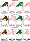 |
Fig. 6. Maps of the Mg II h line profile statistics from the start, middle, and end of the observation. A similar plot for Mg II k may be seen in Fig. A.1. |
4. Forward modelling
We used the 1D non-local thermodynamic equilibrium (NLTE) radiative transfer code PROM (Gouttebroze et al. 1993; Heinzel et al. 1994). In the two introductory PROM papers, the prominence was represented by a 1D slab-like isothermal and isobaric structure suspended in the solar corona with a focus on the six principal hydrogen transitions. Labrosse & Gouttebroze (2004) introduced a prominence-to-corona transition region (PCTR) in order to study the He I triplet lines, which require a PCTR to form. Levens & Labrosse (2019) introduced a Mg II ion to produce the Mg II h&k and Mg II triplet lines, with incident radiation taken from Sun-centre quiet Sun observations by IRIS. The incident radiation is the angle-averaged irradiation on both sides of the prominence. The incident radiation used in this study is that used in Levens & Labrosse (2019), as the grid of models used here is an expansion built on the grid of 1007 models presented in the aforementioned study.
With PROM, we generated a grid of 23 940 models, the parameters of which can be seen in Table 1. These models are a mix of isobaric and isothermal atmospheres and atmospheres containing a PCTR. The terms Tcen and pcen are the central temperature and pressure, respectively; Ttr and ptr are the temperature and pressure at the edge of the PCTR, respectively; slab width is the width of the slab; M is the column mass; H is the height above the solar surface; vT is the microturbulent velocity; vrad is the velocity of the slab parallel to the normal of the solar surface; and γ is a dimensionless number that dictates the extent of the PCTR. For isothermal and isobaric models, there is only one temperature and pressure, T = Tcen and p = pcen. For non-zero values of γ, the higher the value of γ, the steeper the temperature gradient in the PCTR. The PCTR is formulated as a function of column mass (Kippenhahn & Schlüter 1957; Anzer & Heinzel 1999),
 (2)
(2)
 (3)
(3)
Model parameters.
for γ ≥ 2 and where pc = pcen − ptr. A γ value of zero indicates the model is isothermal and isobaric; this is merely a placeholder value and is not used in Eqs. (2) and (3).
Before these model profiles could be matched, they had to first be interpolated down to match the resolution of the IRIS spectrograph. There were two candidates for this interpolation: standard linear and fourth-order weighted essentially non-oscillatory interpolation (WENO4; Janett et al. 2019). Both of these schemes were tested, and they produced similar or identical results. Ultimately, linear was chosen for its expedience. More correctly, one would instead resample the data, but an interpolation is a good approximation.
5. xRMS
The xRMS method is an upgraded version of the rRMS method (Peat et al. 2021). The rRMS method works by measuring the RMS between the models and the whole raster at once by vectorising the problem. A simple one-pixel example of how it works can be seen in Fig. 7. The RMS is measured at every position along the wavelength window, shifting it one pixel at a time. The pixel shift that produces the lowest RMS is selected as the ideal pixel shift for that model. The RMS and associated pixel shift are saved, and then the next model is run. This process is repeated for every model, and the model that produces the lowest RMS from this process is selected as the best model. However, the best-fitting model is not necessarily a good fitting model. For a model to be classified as a “satisfactory match”, its RMS must be below a threshold of 15 000 (Peat et al. 2021).
 |
Fig. 7. How rRMS worked. The orange model profile is rolled over the blue observed profile while measuring the RMS and pixel shift (and consequently Doppler velocity) at every wavelength position. This process has been replaced by a cross-correlation in xRMS. This figure is adapted from Peat (2023). |
However, a cross-correlation is naturally produced when attempting to minimise (or maximise) a mean square (Elliott 1987) and, therefore, also a root mean square. Additionally, Brown et al. (2016) demonstrated the use of a cross-correlation to measure the line core shift of the Lyman lines in solar flares. Since measuring the pixel shift in wavelength space is essentially measuring the line core shift, we could instead use a cross-correlation. Using this approach, we were able to know the ideal pixel shift ahead of time and could skip straight to measuring the RMS at that position only. This improved run time by a factor of ten. However, the models still had to be rolled to their ideal positions, which is a computationally expensive procedure. This was replaced by instead padding the model with zeros and taking slices of the padded array to produce what would be the result of the roll. This resulted in a factor of two increase in speed, giving us an overall improvement of a factor of 20. In Peat et al. (2021), who introduced rRMS, one raster (of the size 32 × 520) for 1007 models had a run-time of approximately 90 min on a dual socket motherboard with two Intel Xeon E5-2697 v4s. With the above-mentioned improvements, xRMS has a run time of approximately 4.5 min under the same conditions. This allowed us to use a model grid of a much greater size. As this approach removes the rolling aspect of rRMS, the improved algorithm was renamed cross RMS (xRMS).
In addition to the increase in speed, an estimate of the error on the recovered thermodynamic properties may be found. To do this, we saved the 20 next-best models after the best model. The choice of 20 was decided in order to fit within the computational limits. With enough memory, xRMS can be asked to hold any arbitrary number of “next-best” models. These models were subject to the RMS threshold. If they were above the RMS threshold, they were discarded. The surviving models were then used to make maps of the thermodynamic properties of those models. These maps were then subtracted from the “best” map, and the map that produced the largest difference was chosen as the error. This was done on a pixel-by-pixel basis, and the model chosen to represent the error in one pixel is not necessarily the same as its neighbouring pixel. These models can be plotted in a similar manner to the diagnostic maps. Pixels that do no have any “next-best” matches have an error of ±0 assigned. To avoid confusion, we assigned any pixels where no “best-match” was found a value of NaN, which is plotted as a bad pixel (white).
6. Results
Figures 8 and 9 show a selection of the diagnostics recovered by xRMS for raster 9. Satisfactory and unsatisfactory matches are both presented in these diagnostic maps for readability, and the maps should be read in tandem with the satisfactory matches plot (see right of Fig. 10). The errors here are given as simple plus-minus errors; however, it is important to note that single ion prominence inversions produce multi-peaked posterior likelihoods (Peat & Osborne, in prep.), so not every number in the stated range is an acceptable value.
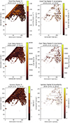 |
Fig. 8. Select diagnostics of the ninth raster of the prominence with their associated fractional errors. The uncertainty plots only show uncertainties where good matches are found. |
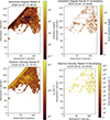 |
Fig. 9. Electron density and ionisation degree of the ninth raster of the prominence with their associated errors. The uncertainty plots only show uncertainties where good matches are found. |
Raster 9 was chosen as our example, as it simply has the greatest number of satisfactory matches, 21.22%. The majority of our satisfactory matches are towards the edges of the prominence, where less fine structure is expected to be observed. As can be seen, the central pressure of the prominence is quite low, remaining below 0.2 dyn cm−2. However, these pixels are unsatisfactory matches (see Fig. 10, right). The uncertainty map shows errors of approximately ±0.2 to ±0.3 dyn cm−2. This could be due to solutions where the effects of pressure can instead be produced by some other parameter.
 |
Fig. 10. Mg II k/h ratio and satisfactory matches. No clear correlation is present. |
The observed central temperatures are rather high compared to typical prominences. Here, we have values ranging from approximately 10 kK to 20 kK. This is consistent with the mean temperatures recovered in our previous study using rRMS (Peat et al. 2021). However, the lower bound found in our previous study was 6 kK. We found errors of up to approximately 5 kK to 15 kK in the areas with good matches. This means the temperature can be up to twice as high or twice as low as that recovered by the best match. This disparity in solutions is likely due to the same reason given for the differences in central pressure. This may demonstrate the degeneracies faced when using a single ion and/or species from 1D prominence modelling to infer the thermodynamic properties (Jejčič et al. 2022; Peat & Osborne, in prep.).
In total, we recovered 14.1% satisfactory matches, 50.3% of which were PCTR models. This is in stark contrast to the 49% satisfactory matches recovered in Peat et al. (2021). The main difference between these two observations is the orientation of the prominence. Here, the line of sight (LOS) is almost parallel with the spine, and in the aforementioned study, the LOS was almost perpendicular to the spine. In the former orientation, we would expect to intercept more fine structure, which can lead to complicated line profiles that 1D prominence modelling cannot effectively reproduce (Gunár et al. 2022; Peat et al. 2023). The gamma plots allowed us to investigate the structure of the PCTR. Where we did find good matches, the gamma factor appears to flip between two, four, and five. The gamma error plot not only shows the uncertainty where a PCTR model is selected as the best fit but also further backs up the flipping nature of the gamma factor, as the uncertainties are between one and three. This shows that there is a relatively gentle PCTR gradient.
As in the previous study, we recovered a large ionisation degree. We used the definition of ionisation degree from Tandberg-Hanssen (1995),
 (4)
(4)
as utilising the commonly used approximations of nH II ≈ ne and nH I ≈ nH0 (where nH0 is the number density of ground state hydrogen) can overestimate nH II by up to 20% (Peat et al. 2021). Our recovered ionisation degree appears quite reasonable, with the largest values appearing at the edges of the prominence material, where one would expect to encounter more of the PCTR. Here, the errors mainly range from ±1 to ±100. The electron density map displays a similar distribution, with more electrons closer to regions that intersect the PCTR. The majority of the structure appears to exhibit an electron density of 1010 cm−3. The majority of the pixels in the uncertainty plot appear to be around ±109 to ±1010 cm−3.
Unlike in Peat et al. (2021), we did not find a weak objective correlation between the areas where we found satisfactory matches and the regions with a high k/h ratio (see Fig. 10). The generally low k/h ratio could also be why the algorithm did not recover many satisfactory matches. In the optically thin regime, the k/h ratio becomes that of the oscillator strengths. The oscillator strengths of Mg II h&k are 0.300 and 0.601, respectively (Theodosiou & Federman 1999), giving a ratio of approximately two. Due to the large amount of potential fine structure along the LOS, it is likely that the best matches are found where the optical thickness is the highest, as this is where we only observed the “front-most” structure. However, due to the scattering of incident radiation, the k/h ratio can exceed two in solar prominences (Heinzel 2023, priv. comm.). Therefore, this may not be a reliable measurement of the optical thickness.
7. Conclusions
The prominence of 1 October 2019 was very dynamic, with one large flow observed towards the solar limb. From the line statistics recovered via the quantile method, we found the prominence to contain a mixture of asymmetries between 0.8 and –0.8. It was fairly dynamic, with recovered LOS velocities of up to 70 km s−1. Through the use of the new xRMS algorithm, we found central temperatures of 10 kK to 20 kK and central pressures of 0.2 dyn cm−2. The ionisation degree was found to range from around 1 to 100, with an electron density of mainly 1010 cm−3. The range of the associated uncertainties recovered via this new method are quite large, an order of magnitude so. This is likely an example of the degeneracies faced when using single ion and/or species 1D prominence inversions (Jejčič et al. 2022; Peat & Osborne, in prep.). In future work, the algorithm should be expanded to have the ability to match several co-aligned observations in different ion and/or species (e.g. Mg II h&k and Hα) to attempt to constrain these degenerate solutions. Additionally, prominences showing higher k/h ratios and/or oriented perpendicular to the LOS may also be better candidates for this method.
Available at https://github.com/OfAaron3/irispreppy or via pip.
Acknowledgments
A.W.P. acknowledges financial support from STFC via grant ST/S505390/1. N.L. acknowledges support from STFC grant ST/T000422/1. We would also like to thank Dr Graham S. Kerr for supplying the IRIS spatial PSFs and Dr Christopher M. J. Osborne for writing the Python implementation of WENO4. IRIS is a NASA small explorer mission developed and operated by LMSAL with mission operations executed at NASA Ames Research Center and major contributions to downlink communications funded by ESA and the Norwegian Space Centre. AIA data courtesy of NASA/SDO and the AIA, EVE, and HMI science teams. Hinode is a Japanese mission developed and launched by ISAS/JAXA, collaborating with NAOJ as a domestic partner, NASA and STFC (UK) as international partners. Scientific operation of the Hinode mission is conducted by the Hinode science team organized at ISAS/JAXA. This team mainly consists of scientists from institutes in the partner countries. Support for the post-launch operation is provided by JAXA and NAOJ (Japan), STFC (UK), NASA (USA), ESA, and NSC (Norway). This research used version 3.7.1 of Matplotlib (Hunter 2007), version 1.24.3 of NumPy (Harris et al. 2020), version 1.10.1 of SciPy (Virtanen et al. 2020), version 4.1.5 of the SunPy open source software package (Barnes et al. 2020b), version 0.7.3 of the aiapy open source software package (Barnes et al. 2020a), and version 5.2.2 of Astropy (http://www.astropy.org) a community-developed core Python package for Astronomy (Astropy Collaboration 2013, 2018).
References
- Anzer, U., & Heinzel, P. 1999, A&A, 349, 974 [NASA ADS] [Google Scholar]
- Aschwanden, M. J. 2004, in Physics of the Solar Corona: An Introduction, Springer-Praxis Books in Geophysical Sciences, (Berlin; New York: Springer) [Google Scholar]
- Astropy Collaboration (Robitaille, T. P., et al.) 2013, A&A, 558, A33 [NASA ADS] [CrossRef] [EDP Sciences] [Google Scholar]
- Astropy Collaboration (Price-Whelan, A. M., et al.) 2018, AJ, 156, 123 [Google Scholar]
- Barczynski, K., Schmieder, B., Gelly, B., Peat, A. W., & Labrosse, N. 2023, A&A, 680, A63 [NASA ADS] [CrossRef] [EDP Sciences] [Google Scholar]
- Barnes, W. T., Cheung, M. C. M., Bobra, M. G., et al. 2020a, J. Open Source Softw., 5, 2801 [NASA ADS] [CrossRef] [Google Scholar]
- Barnes, W. T., Bobra, M. G., Christe, S. D., et al. 2020b, ApJ, 890, 68 [Google Scholar]
- Brown, S. A., Fletcher, L., & Labrosse, N. 2016, A&A, 596, A51 [NASA ADS] [CrossRef] [EDP Sciences] [Google Scholar]
- De Pontieu, B., Title, A. M., Lemen, J. R., et al. 2014, Sol. Phys., 289, 2733 [Google Scholar]
- Domingo, V., Fleck, B., & Poland, A. I. 1995, Space Sci. Rev., 72, 81 [Google Scholar]
- Elliott, D. F., ed. 1987, Handbook of Digital Signal Processing: Engineering Applications (San Diego: Academic Press) [Google Scholar]
- Freeland, S. L., & Handy, B. N. 1998, Sol. Phys., 182, 497 [Google Scholar]
- Gardner, M. 1970, Sci. Am., 223, 120 [NASA ADS] [CrossRef] [Google Scholar]
- Golub, L., DeLuca, E., Austin, G., et al. 2007, Sol. Phys., 243, 63 [NASA ADS] [CrossRef] [Google Scholar]
- Gouttebroze, P., Heinzel, P., & Vial, J.-C. 1993, A&AS, 99, 513 [NASA ADS] [Google Scholar]
- Gunár, S., Heinzel, P., Koza, J., & Schwartz, P. 2022, ApJ, 934, 133 [CrossRef] [Google Scholar]
- Harris, C. R., Millman, K. J., van der Walt, S. J., et al. 2020, Nature, 585, 357 [NASA ADS] [CrossRef] [Google Scholar]
- Heinzel, P., Gouttebroze, P., & Vial, J.-C. 1994, A&A, 292, 656 [NASA ADS] [Google Scholar]
- Heinzel, P., Schmieder, B., Vial, J. C., & Kotrč, P. 2001, A&A, 370, 281 [NASA ADS] [CrossRef] [EDP Sciences] [Google Scholar]
- Hirayama, T. 1971, Sol. Phys., 17, 50 [NASA ADS] [CrossRef] [Google Scholar]
- Hirayama, T. 1985, Sol. Phys., 100, 415 [NASA ADS] [CrossRef] [Google Scholar]
- Hunter, J. D. 2007, Comp. Sci. Eng., 9, 90 [NASA ADS] [CrossRef] [Google Scholar]
- Janett, G., Steiner, O., Alsina Ballester, E., Belluzzi, L., & Mishra, S. 2019, A&A, 624, A104 [NASA ADS] [CrossRef] [EDP Sciences] [Google Scholar]
- Jejčič, S., Heinzel, P., Schmieder, B., et al. 2022, ApJ, 932, 3 [CrossRef] [Google Scholar]
- Kerr, G. S., Simões, P. J. A., Qiu, J., & Fletcher, L. 2015, A&A, 582, A50 [NASA ADS] [CrossRef] [EDP Sciences] [Google Scholar]
- Kippenhahn, R., & Schlüter, A. 1957, Z. Astrophys., 43, 36 [Google Scholar]
- Kosugi, T., Matsuzaki, K., Sakao, T., et al. 2007, Sol. Phys., 243, 3 [Google Scholar]
- Labrosse, N., & Gouttebroze, P. 2004, ApJ, 617, 614 [NASA ADS] [CrossRef] [Google Scholar]
- Lemen, J. R., Title, A. M., Akin, D. J., et al. 2012, Sol. Phys., 275, 17 [Google Scholar]
- Levens, P. J., & Labrosse, N. 2019, A&A, 625, A30 [NASA ADS] [CrossRef] [EDP Sciences] [Google Scholar]
- Mein, P., & Rayrole, J. 1985, Vistas Astron., 28, 567 [NASA ADS] [CrossRef] [Google Scholar]
- Parenti, S., Schmieder, B., Heinzel, P., & Golub, L. 2012, ApJ, 754, 66 [Google Scholar]
- Peat, A. W. 2023, Ph.D. Thesis, University of Glasgow, UK [Google Scholar]
- Peat, A. W., Labrosse, N., Schmieder, B., & Barczynski, K. 2021, A&A, 653, A5 [NASA ADS] [CrossRef] [EDP Sciences] [Google Scholar]
- Peat, A. W., Labrosse, N., & Gouttebroze, P. 2023, A&A, 679, A156 [NASA ADS] [CrossRef] [EDP Sciences] [Google Scholar]
- Pesnell, W. D., Thompson, B. J., & Chamberlin, P. C. 2012, Sol. Phys., 275, 3 [Google Scholar]
- Ruan, G., Schmieder, B., Mein, P., et al. 2018, ApJ, 865, 123 [NASA ADS] [CrossRef] [Google Scholar]
- Ruan, G., Jejčič, S., Schmieder, B., et al. 2019, ApJ, 886, 134 [NASA ADS] [CrossRef] [Google Scholar]
- Tandberg-Hanssen, E. 1995, in The Nature of Solar Prominences (Dordrecht: Springer Netherlands), Astrophys. Space Sci. Lib., 199 [Google Scholar]
- Theodosiou, C. E., & Federman, S. R. 1999, ApJ, 527, 470 [NASA ADS] [CrossRef] [Google Scholar]
- Virtanen, P., Gommers, R., Oliphant, T. E., et al. 2020, Nat. Methods, 17, 261 [Google Scholar]
- Wilhelm, K., Curdt, W., Marsch, E., et al. 1995, Sol. Phys., 162, 189 [Google Scholar]
- Zhang, P., Buchlin, É., & Vial, J.-C. 2019, A&A, 624, A72 [NASA ADS] [CrossRef] [EDP Sciences] [Google Scholar]
Appendix A: Mg II k statistic maps
All Tables
All Figures
 |
Fig. 1. Prominence as it appeared as a filament in Hα on 28 September 2019. The filament is highlighted with a red circle. |
| In the text | |
 |
Fig. 2. Configuration of this coordinated observation. The pointing of THEMIS is not trivial to determine, so it is omitted from this plot. |
| In the text | |
 |
Fig. 3. Hinode/XRT Al Poly/Open filter observations. The coronal cavity is clearly visible around 700″, –800″. |
| In the text | |
 |
Fig. 4. Beginning, middle, and end (from left to right) of the IRIS prominence observation. The top, middle, and bottom rows are Mg II k, 304 Å and 171 Å, respectively. The prominence appears far more extended in Mg II k than in 304 Å, but the IRIS/SJI FOV does not cover the entire structure as AIA does. Notably, 171 Å allows us to see the high temperature PCTR that shrouds the structure. |
| In the text | |
 |
Fig. 5. Examples of red (left) and blue (right) asymmetry. The intensities here are measured in 104 erg s−1 cm−2 Å−1 sr−1. |
| In the text | |
 |
Fig. 6. Maps of the Mg II h line profile statistics from the start, middle, and end of the observation. A similar plot for Mg II k may be seen in Fig. A.1. |
| In the text | |
 |
Fig. 7. How rRMS worked. The orange model profile is rolled over the blue observed profile while measuring the RMS and pixel shift (and consequently Doppler velocity) at every wavelength position. This process has been replaced by a cross-correlation in xRMS. This figure is adapted from Peat (2023). |
| In the text | |
 |
Fig. 8. Select diagnostics of the ninth raster of the prominence with their associated fractional errors. The uncertainty plots only show uncertainties where good matches are found. |
| In the text | |
 |
Fig. 9. Electron density and ionisation degree of the ninth raster of the prominence with their associated errors. The uncertainty plots only show uncertainties where good matches are found. |
| In the text | |
 |
Fig. 10. Mg II k/h ratio and satisfactory matches. No clear correlation is present. |
| In the text | |
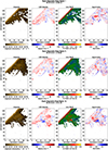 |
Fig. A.1. Same as Fig. 6 but for Mg II k. |
| In the text | |
Current usage metrics show cumulative count of Article Views (full-text article views including HTML views, PDF and ePub downloads, according to the available data) and Abstracts Views on Vision4Press platform.
Data correspond to usage on the plateform after 2015. The current usage metrics is available 48-96 hours after online publication and is updated daily on week days.
Initial download of the metrics may take a while.


